
A Worrying Future for River Flows in the Brazilian Cerrado Provoked by Land Use and Climate Changes
 , , , , , and
Abstract
:1. Introduction
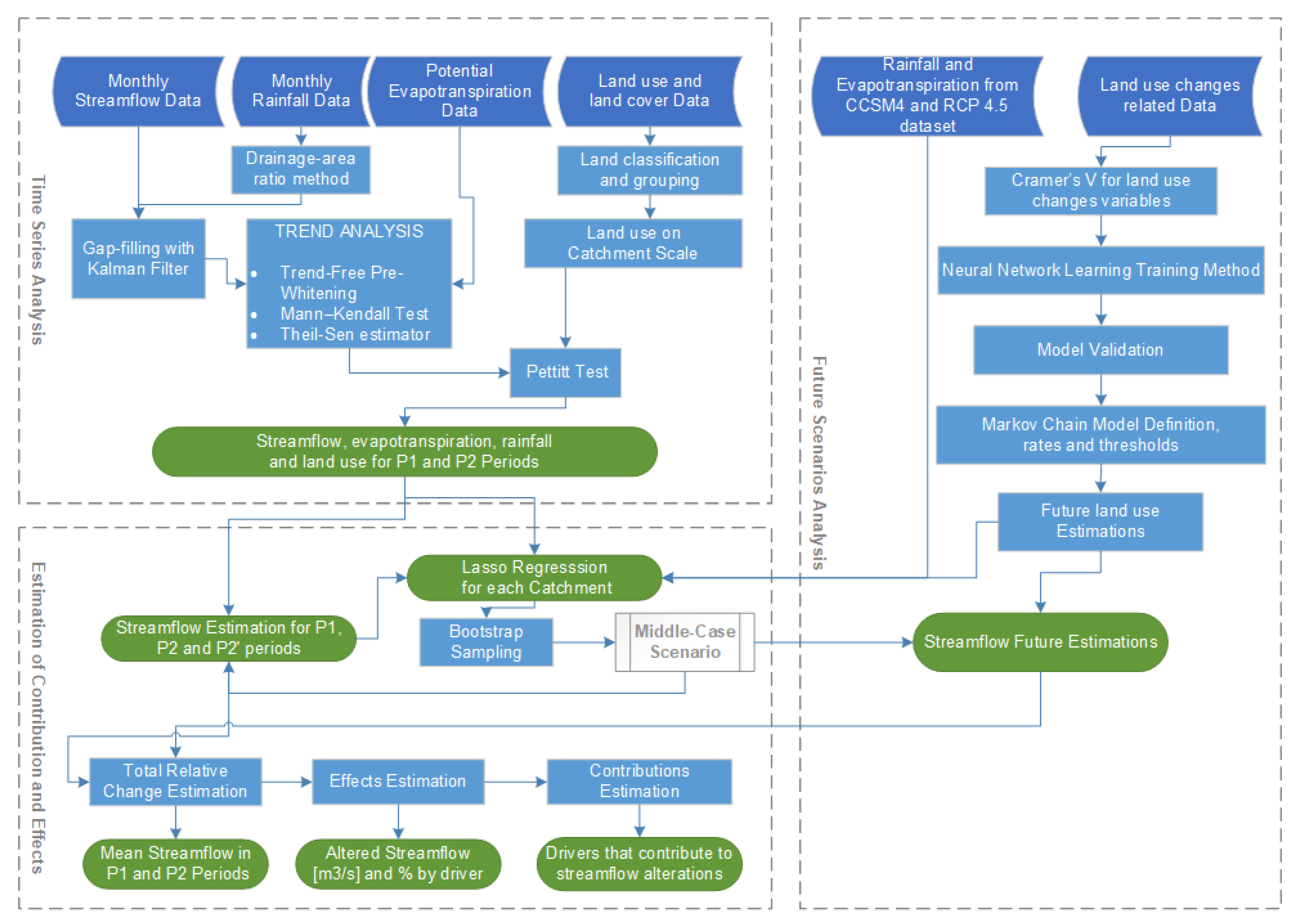
2. Materials and Methods
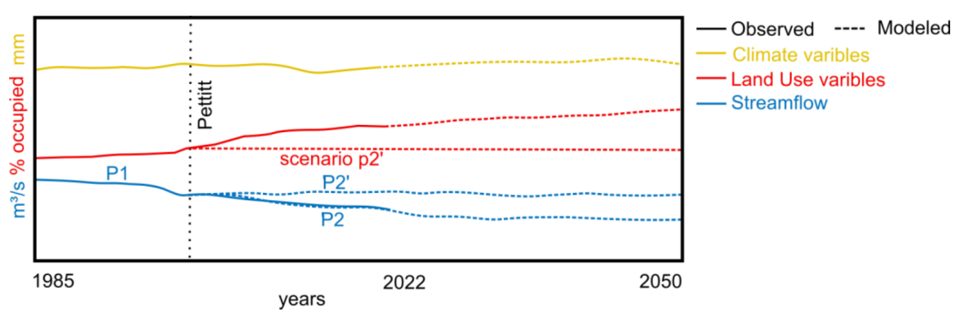
2.1. Time Series Analyses
2.2. Estimate of Contribution and Effects
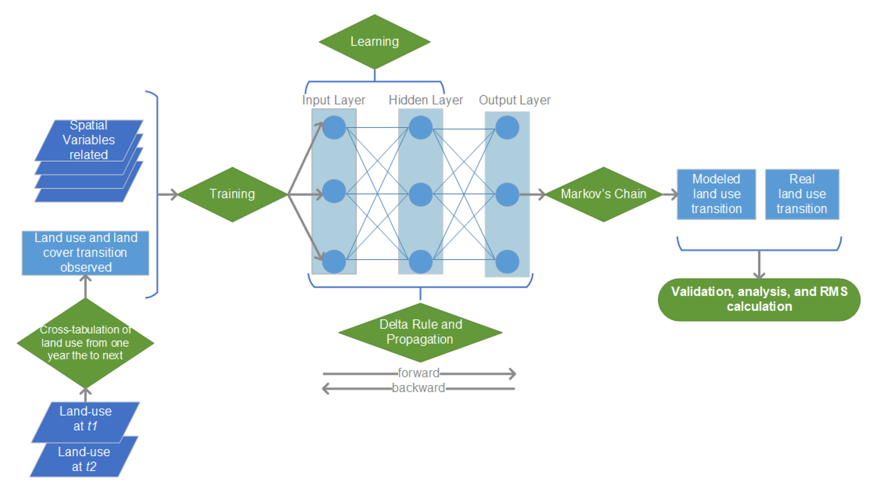
2.3. Future Land Use and Climate Change Scenarios
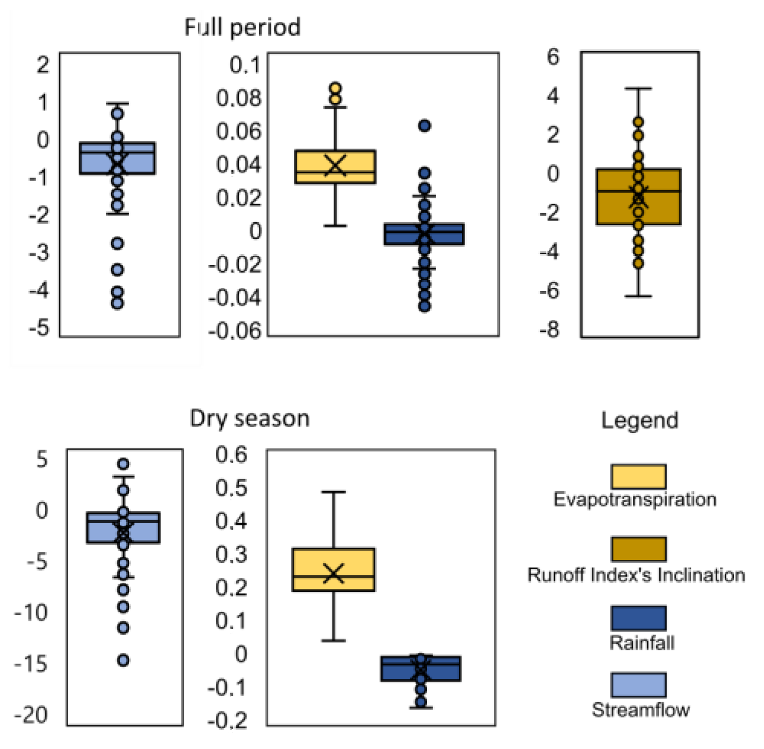
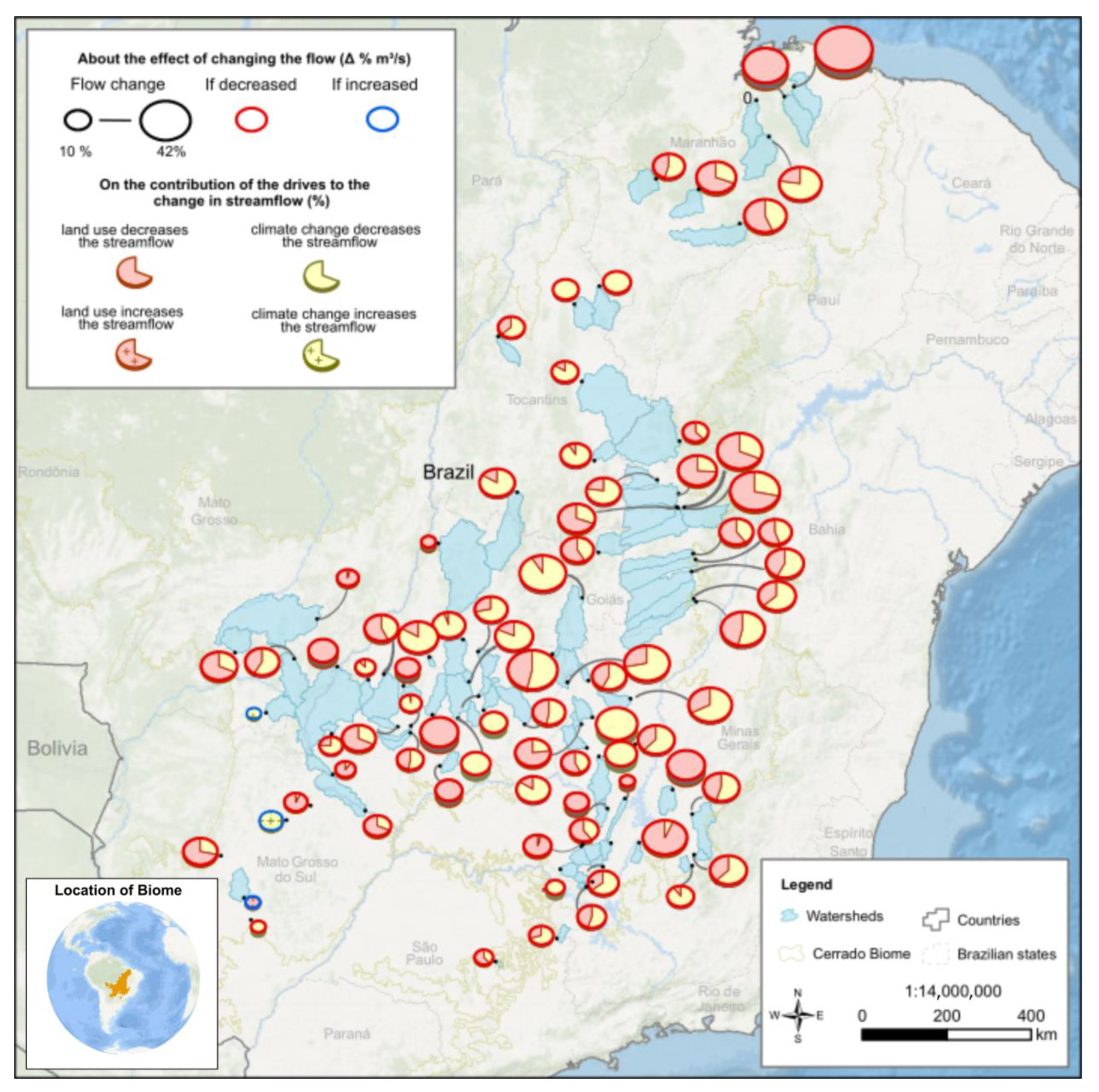
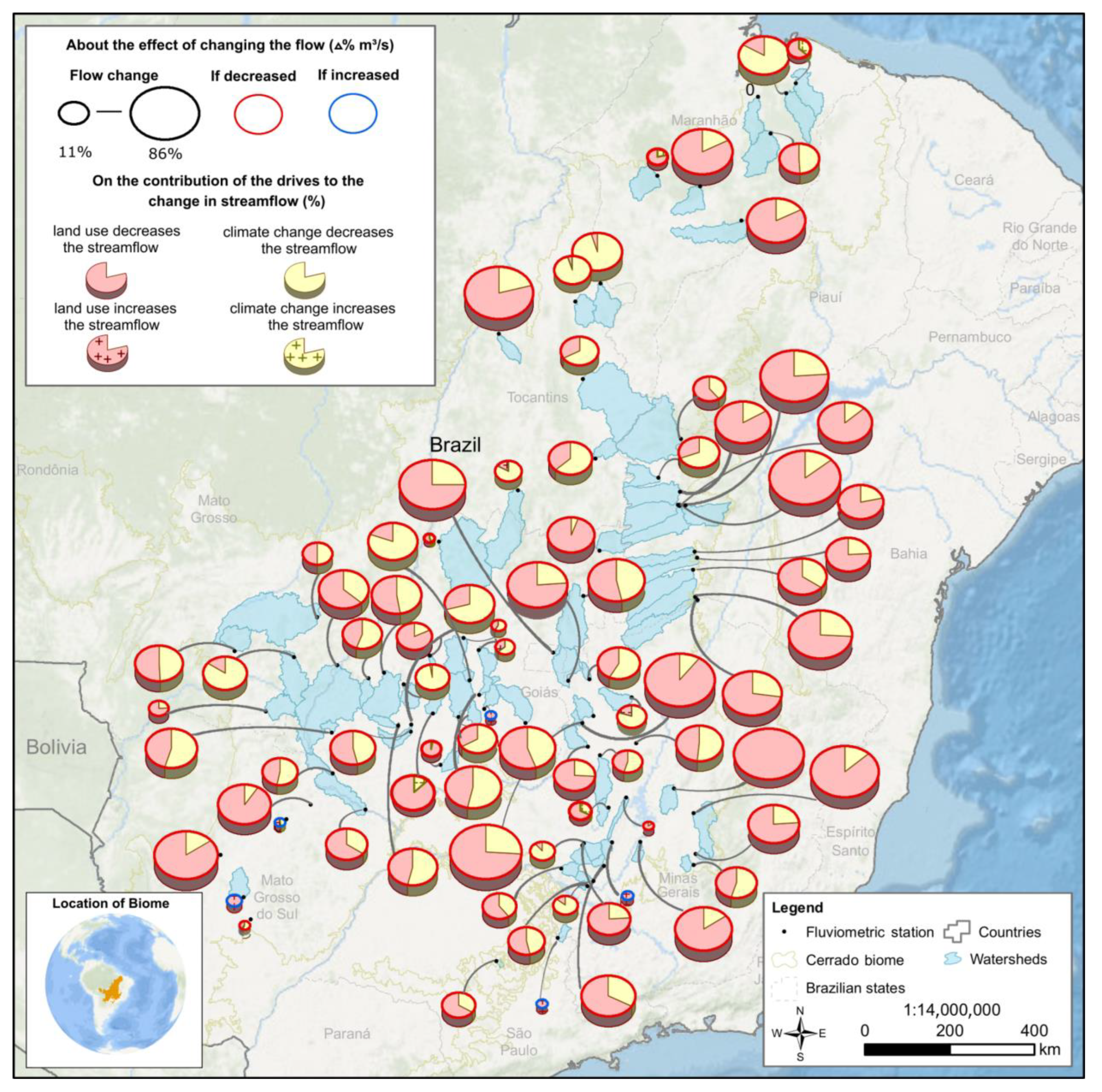
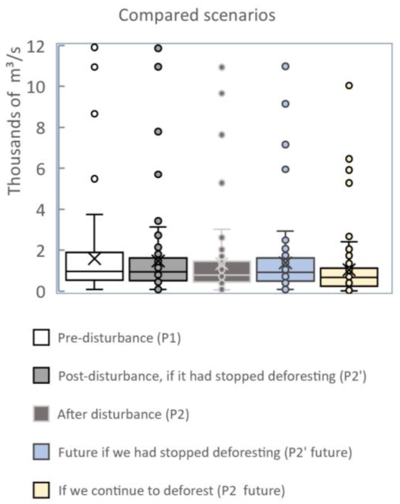
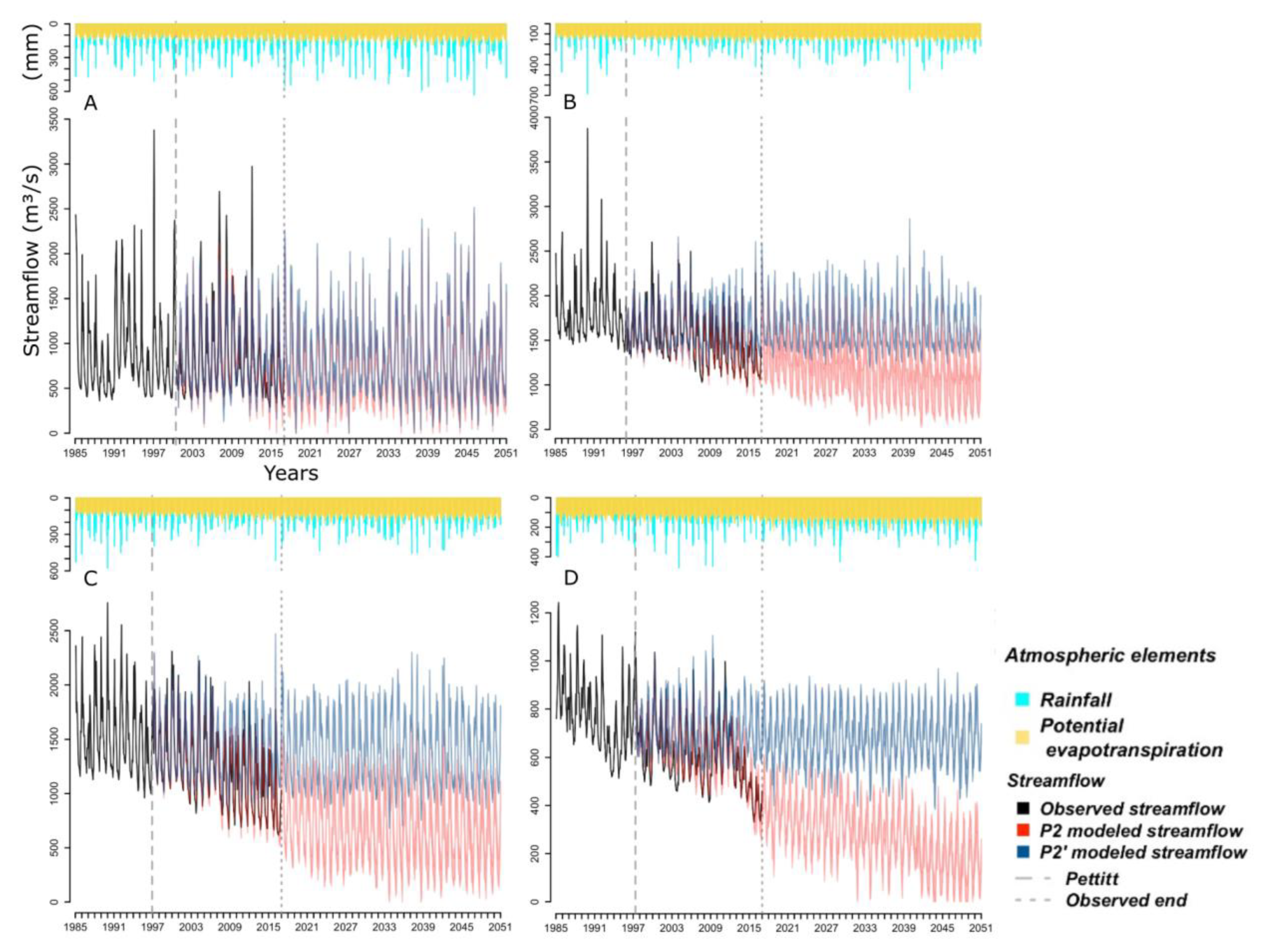
3. Results
4. Discussion
5. Conclusions
Author Contributions
Funding
Informed Consent Statement
Data Availability Statement
Acknowledgments
Conflicts of Interest
References
- Hoekstra, A.Y.; Hung, P.Q. Virtual Water Trade a Quantification of Virtual Water Flows between Nations in Relation to International Crop Trade; IHE Delft: Delft, The Netherlands, 2002; pp. 1–120. Available online: https://waterfootprint.org/media/downloads/Report11.pdf (accessed on 10 January 2020).
- Langenbrunner, B. Water, water not everywhere. Nat. Clim. Chang. 2021, 11, 650. [Google Scholar] [CrossRef]
- Ashok Mishra, P.D. Separating the impacts of climate change and human activities on streamflow: A review of methodologies and critical assumptions. J. Hydrol. 2017, 548, 278–290. [Google Scholar]
- Sano, E.E.; Rosa, R.; Brito, J.L.S.; Ferreira, L.G. Mapeamento semidetalhado do uso da terra do Bioma Cerrado. Pesqui. Agropecu. Bras. 2008, 43, 153–156. [Google Scholar] [CrossRef]
- Denis Castilho, M.P. Cerrados Perspectivas e Olhares; Vieira: Goiânia, Brazil, 2010. [Google Scholar]
- Trase Yearbook 2020—The State of Forest Risk Supply Chains, Brazilian Soybean. 2020. Available online: https://insights.trase.earth/yearbook/contexts/brazil-soy/ (accessed on 5 July 2021).
- Jepson, W.; Brannstrom, C.; Filippi, A. Access Regimes and Regional Land Change in the Brazilian Cerrado, 1972–2002. Ann. Assoc. Am. Geogr. 2010, 100, 87–111. [Google Scholar] [CrossRef]
- Mapbiomas Collection 4. 2020. Available online: https://mapbiomas.org/ (accessed on 1 July 2020).
- Trase. Trase Yearbook 2020—The State of Forest Risk Supply Chains, Brazilian Beef. 2020. Available online: https://insights.trase.earth/yearbook/contexts/brazil-beef (accessed on 20 November 2020).
- IBGE. Produção Agrícola Municipal. 2020. Available online: https://sidra.ibge.gov.br/pesquisa/pam/tabelas (accessed on 2 November 2020).
- FAO. World Agriculture: Towards 2015/2030. 2002. Available online: https://www.fao.org/3/y3557e/y3557e06.htm (accessed on 19 November 2019).
- IPEA. Boletim de Taxa de Cambio. 2022. Available online: http://www.ipeadata.gov.br/ExibeSerie.aspx?serid=31924 (accessed on 29 July 2022).
- Pereira, E.J.D.A.L.; Ribeiro, L.C.D.S.; Freitas, L.F.D.S.; Pereira, H.B.D.B. Brazilian policy and agribusiness damage the Amazon rainforest. Land Use Policy 2020, 92, 104491. [Google Scholar] [CrossRef]
- Sauer, S. Soy expansion into the agricultural frontiers of the Brazilian Amazon: The agribusiness economy and its social and environmental conflicts. Land Use Policy 2018, 79, 326–338. [Google Scholar] [CrossRef]
- Myers, N.; Mittermeier, R.A.; Mittermeier, C.G.; da Fonseca, G.A.B.; Kent, J. Biodiversity hotspots for conservation priorities. Nature 2000, 403, 853–858. [Google Scholar] [CrossRef]
- Sano, S.M.; Almeida, S.P.d.A.; Ribeiro, J.F. Cerrado: Ecologia e Flora; Embrapa: Brasília, Brazil, 2008; Volume 1. [Google Scholar]
- Almagro, A.; Oliveira, P.T.S.; Neto, A.A.M.; Roy, T.; Troch, P. CABra: A novel large-sample dataset for Brazilian catchments. Hydrol. Earth Syst. Sci. 2021, 25, 3105–3135. [Google Scholar] [CrossRef]
- Silva, A.; Souza, S.; Filho, O.C.; Eloy, L.; Salmona, Y.; Passos, C. Water Appropriation on the Agricultural Frontier in Western Bahia and Its Contribution to Streamflow Reduction: Revisiting the Debate in the Brazilian Cerrado. Water 2021, 13, 1054. [Google Scholar] [CrossRef]
- Spera, S.A.; Galford, G.L.; Coe, M.T.; Macedo, M.N.; Mustard, J.F. Land-use change affects water recycling in Brazil’s last agricultural frontier. Glob. Chang. Biol. 2016, 22, 3405–3413. [Google Scholar] [CrossRef]
- Nóbrega, R.L.B.; Guzha, A.C.; Torres, G.N.; Kovacs, K.; Lamparter, G.; Amorim, R.S.S.; Couto, E.; Gerold, G. Effects of conversion of native cerrado vegetation to pasture on soil hydro-physical properties, evapotranspiration and streamflow on the Amazonian agricultural frontier. PLoS ONE 2017, 12, e0179414. [Google Scholar] [CrossRef] [PubMed] [Green Version]
- Gonçalves, R.D.; Engelbrecht, B.Z.; Chang, H.K. Análise hidrológica de séries históricas da Bacia do Rio Grande (BA): Contribuição do Sistema Aquífero Urucuia. Águas Subterrâneas 2016, 30, 190. [Google Scholar] [CrossRef] [Green Version]
- Dias, L.C.P.; Macedo, M.N.; Costa, M.H.; Coe, M.T.; Neill, C. Effects of land cover change on evapotranspiration and streamflow of small catchments in the Upper Xingu River Basin, Central Brazil. J. Hydrol. Reg. Stud. 2015, 4, 108–122. [Google Scholar] [CrossRef] [Green Version]
- Marengo, J.A.; Alves, L.M. Tendências hidrológicas da bacia do rio Paraíba do Sul. Rev. Bras. Meteorol. 2005, 20, 215–226. [Google Scholar]
- Pousa, R.; Costa, M.H.; Pimenta, F.M.; Fontes, V.C.; De Brito, V.F.A.; Castro, M. Climate Change and Intense Irrigation Growth in Western Bahia, Brazil: The Urgent Need for Hydroclimatic Monitoring. Water 2019, 11, 933. [Google Scholar] [CrossRef] [Green Version]
- Favareto, A.; Nakagawa, L.; Pó, M.; Seifer, P.; Kleeb, S. Entre Chapadas e Baixões do Matopiba: Dinâmicas Territoriais e Impactos Socioeconômicos Na Fronteira da Expansão Agropecuária. Prefixo Editor. 2019, 8, 92545. [Google Scholar]
- Os Pivôs da Discórdia e a Digna Raiva: Uma Análise dos Conflitos por Terra, Água e Território em Correntina—BA. Doc. De Trab. Inédito 2018.
- Strassburg, B.B.N.; Brooks, T.; Feltran-Barbieri, R.; Iribarrem, A.; Crouzeilles, R.; Loyola, R.; Latawiec, A.E.; Filho, F.J.B.O.; Scaramuzza, C.A.D.M.; Scarano, F.R.; et al. Moment of truth for the Cerrado hotspot. Nat. Ecol. Evol. 2017, 1, 99. [Google Scholar] [CrossRef]
- Oliveira, P.T.S.; Wendland, E.; Nearing, M.A.; Scott, R.L.; Rosolem, R.; da Rocha, H.R. The water balance components of undisturbed tropical woodlands in the Brazilian cerrado. Hydrol. Earth Syst. Sci. 2015, 19, 2899–2910. [Google Scholar] [CrossRef] [Green Version]
- Marengo, J.A.; Jimenez, J.C.; Espinoza, J.-C.; Cunha, A.P.; Aragão, L.E.O. Increased climate pressure on the agricultural frontier in the Eastern Amazonia–Cerrado transition zone. Sci. Rep. 2022, 12, 457. [Google Scholar] [CrossRef]
- Soterroni, A.C.; Ramos, F.M.; Mosnier, A.; Fargione, J.; Andrade, P.R.; Baumgarten, L.; Pirker, J.; Obersteiner, M.; Kraxner, F.; Câmara, G.; et al. Expanding the Soy Moratorium to Brazil’s Cerrado. Sci. Adv. 2019, 5, eaav7336. [Google Scholar] [CrossRef] [Green Version]
- Timpe, K.; Kaplan, D. The changing hydrology of a dammed Amazon. Sci. Adv. 2017, 3, e1700611. [Google Scholar] [CrossRef] [Green Version]
- Arora, V.K. The use of the aridity index to assess climate change effect on annual runoff. J. Hydrol. 2002, 265, 164–177. [Google Scholar] [CrossRef]
- Luo, X.; Li, H.-Y.; Leung, L.R.; Tesfa, T.K.; Getirana, A.; Papa, F.; Hess, L.L. Modeling surface water dynamics in the Amazon Basin using MOSART-Inundation v1.0: Impacts of geomorphological parameters and river flow representation. Geosci. Model Dev. 2017, 10, 1233–1259. [Google Scholar] [CrossRef] [Green Version]
- Calijuri, M.L.; Castro, J.D.S.; Costa, L.S.; Assemany, P.P.; Alves, J.E.M. Impact of land use/land cover changes on water quality and hydrological behavior of an agricultural subwatershed. Environ. Earth Sci. 2015, 74, 5373–5382. [Google Scholar] [CrossRef]
- Li, C.; Wang, L.; Wanrui, W.; Qi, J.; Linshan, Y.; Zhang, Y.; Lei, W.; Cui, X.; Wang, P. An analytical approach to separate climate and human contributions to basin streamflow variability. J. Hydrol. 2018, 559, 30–42. [Google Scholar] [CrossRef]
- Kalman, R.E. A New Approach to Linear Filtering and Prediction Problems. J. Basic Eng. 1960, 82, 35–45. [Google Scholar] [CrossRef] [Green Version]
- Chui, C.K.; Chen, G. Kalman Filtering with Real-Time Applications; Springer: Berlin, Germany, 2009. [Google Scholar]
- Li, J.; Heap, A.D. A review of comparative studies of spatial interpolation methods in environmental sciences: Performance and impact factors. Ecol. Inform. 2011, 6, 228–241. [Google Scholar] [CrossRef]
- Xavier, A.C.; King, C.W.; Scanlon, B.R. Daily gridded meteorological variables in Brazil (1980–2013). Int. J. Climatol. 2016, 36, 2644–2659. [Google Scholar] [CrossRef] [Green Version]
- Tibshirani, R. Regression Shrinkage and Selection Via the Lasso. J. R. Stat. Soc. Ser. B Methodol. 1996, 58, 267–288. [Google Scholar] [CrossRef]
- Pettitt, A.N. A Non-Parametric Approach to the Change-Point Problem. J. R. Stat. Soc. Ser. C (Appl. Stat.) 1979, 28, 126–135. [Google Scholar] [CrossRef]
- Bradley, J.V. Distribution-Free Statistical Tests; United States Air Force: Washington, DC, USA, 1968. [Google Scholar]
- Thom, H.C.S. Same Methods of Climatological Analyses; World Meteorological Organization: Geneva, Switzerland, 1966; p. 16. [Google Scholar]
- Sen, P.K. Estimates of the Regression Coefficient Based on Kendall’s Tau. J. Am. Stat. Assoc. 1968, 63, 1379–1389. [Google Scholar] [CrossRef]
- Rosin, C.; Amorim, R.; Morais, T. Análise de tendências hidrológicas na bacia do rio das Mortes/analysis of hydrological trends in the Rio das Mortes watershed. Rev. Bras. Recur. Hídricos 2015, 20, 991–998. [Google Scholar] [CrossRef]
- Sriwongsitanon, N.; Taesombat, W. Effects of land cover on runoff coefficient. J. Hydrol. 2011, 410, 226–238. [Google Scholar] [CrossRef]
- Hastie, T.; Tibshirani, R.; Friedman, J.H. The Elements of Statistical Learning: Data Mining, Inference, and Prediction; Springer: Berlin/Heidelberg, Germany, 2009. [Google Scholar]
- Duan, Q.; Sorooshian, S.; Gupta, V. Effective and efficient global optimization for conceptual rainfall-runoff models. Water Resour. Res. 1992, 28, 1015–1031. [Google Scholar] [CrossRef]
- Zhang, J.; Zhang, Y.; Song, J.; Cheng, L. Evaluating relative merits of four baseflow separation methods in Eastern Australia. J. Hydrol. 2017, 549, 252–263. [Google Scholar] [CrossRef]
- Clark Labs. The Land Change Modeler for Ecological Sustainability. IDRISI Focus Pap. 2007, 2, 234–256. [Google Scholar]
- Eastman, J.R. IDRISI Taiga Guide to GIS and Image Processing; Clark Labs Clark University: Worcester, MA, USA, 2009. [Google Scholar]
- Rajão, R.; Nobre, A.D.; Cunha, E.L.; Duarte, T.R.; Marcolino, C.; Soares-Filho, B.; Sparovek, G.; Rodrigues, R.R.; Valera, C.; Bustamante, M.; et al. The risk of fake controversies for Brazilian environmental policies. Biol. Conserv. 2022, 266, 109447. [Google Scholar] [CrossRef]
- Azevedo, A.A.; Saito, C.H. O perfil dos desmatamentos em Mato Grosso, após implementação do licenciamento ambiental em propriedades rurais. CERNE 2013, 19, 111–122. [Google Scholar] [CrossRef] [Green Version]
- Françoso, R.D.; Brandão, R.; Nogueira, C.C.; Salmona, Y.B.; Machado, R.B.; Colli, G.R. Habitat loss and the effectiveness of protected areas in the Cerrado Biodiversity Hotspot. Nat. Conserv. 2015, 13, 35–40. [Google Scholar] [CrossRef] [Green Version]
- Clark Labs. Land Change Modeler: An Application within IDRISI for Analyzing and Predicting Land Cover Change and Assessing the Implications of that Change for Biodiversity. Available online: https://clarklabs.org/terrset/land-change-modeler/ (accessed on 30 January 2023).
- Almeida, C.M.; Gleriani, J.M.; Castejon, E.F.; Soares-Filho, B.S. Using neural networks and cellular automata for modelling intra-urban land-use dynamics. Int. J. Geogr. Inf. Sci. 2008, 22, 943–963. [Google Scholar] [CrossRef]
- Pontius, R.; Huffaker, D.; Denman, K. Useful techniques of validation for spatially explicit land-change models. Ecol. Model. 2004, 179, 445–461. [Google Scholar] [CrossRef]
- Pontius Júnior, R.G.; Chen, H. GEOMOD Modeling Land-Use & Cover Change Modeling; Clark University: Worcester, MA, USA, 2006; 44p. [Google Scholar]
- Thrasher, B.; Maurer, E.P.; McKellar, C.; Duffy, P.B. Technical Note: Bias correcting climate model simulated daily temperature extremes with quantile mapping. Hydrol. Earth Syst. Sci. 2012, 16, 3309–3314. [Google Scholar] [CrossRef] [Green Version]
- Avila-Diaz, A.; Benezoli, V.; Justino, F.; Torres, R.; Wilson, A. Assessing current and future trends of climate extremes across Brazil based on reanalyses and earth system model projections. Clim. Dyn. 2020, 55, 1403–1426. [Google Scholar] [CrossRef]
- Avila-Diaz, A.; Abrahão, G.; Justino, F.; Torres, R.; Wilson, A. Extreme climate indices in Brazil: Evaluation of downscaled earth system models at high horizontal resolution. Clim. Dyn. 2020, 54, 5065–5088. [Google Scholar] [CrossRef]
- Salviano, M.F.; Groppo, J.D.; Pellegrino, G.Q. Análise de Tendências em Dados de Precipitação e Temperatura no Brasil. Rev. Bras. Meteorol. 2016, 31, 64–73. [Google Scholar] [CrossRef] [Green Version]
- Patterson, L.A.; Lutz, B.; Doyle, M.W. Climate and direct human contributions to changes in mean annual streamflow in the South Atlantic, USA. Water Resour. Res. 2013, 49, 7278–7291. [Google Scholar] [CrossRef]
- Zhou, G.; Wei, X.; Chen, X.; Zhou, P.; Liu, X.; Xiao, Y.; Sun, G.; Scott, D.F.; Zhou, S.; Han, L.; et al. Global pattern for the effect of climate and land cover on water yield. Nat. Commun. 2015, 6, 5918. [Google Scholar] [CrossRef] [Green Version]
- Zhang, M.; Liu, N.; Harper, R.; Li, Q.; Liu, K.; Wei, X.; Ning, D.; Hou, Y.; Liu, S. A global review on hydrological responses to forest change across multiple spatial scales: Importance of scale, climate, forest type and hydrological regime. J. Hydrol. 2017, 546, 44–59. [Google Scholar] [CrossRef] [Green Version]
- Creed, I.F.; Noordwijk, M. Forest and Water on a Changing Planet: Vulnerability, Adaptation and Governance Opportunities; International Union of Forestry Research Organizations—IUFRO: Viena, Austria, 2018; Volume 38, 188p, Available online: https://www.cabdirect.org/cabdirect/abstract/20193124755 (accessed on 12 November 2020).
- Coble, A.A.; Barnard, H.; Du, E.; Johnson, S.; Jones, J.; Keppeler, E.; Kwon, H.; Link, T.E.; Penaluna, B.E.; Reiter, M.; et al. Long-term hydrological response to forest harvest during seasonal low flow: Potential implications for current forest practices. Sci. Total. Environ. 2020, 730, 138926. [Google Scholar] [CrossRef]
- Wierik, S.A.T.; Cammeraat, E.L.H.; Gupta, J.; Artzy-Randrup, Y.A. Reviewing the Impact of Land Use and Land-Use Change on Moisture Recycling and Precipitation Patterns. Water Resour. Res. 2021, 57, e2020WR029234. [Google Scholar] [CrossRef]
- Zhao, F.; Zhang, L.; Xu, Z.; Scott, D.F. Evaluation of methods for estimating the effects of vegetation change and climate variability on streamflow: Effects of vegetation and climate variability. Water Resour. Res. 2010, 46, W03505. [Google Scholar] [CrossRef]
- Brown, A.E.; Zhang, L.; McMahon, T.A.; Western, A.W.; Vertessy, R.A. A review of paired catchment studies for determining changes in water yield resulting from alterations in vegetation. J. Hydrol. 2005, 310, 28–61. [Google Scholar] [CrossRef]
- Levy, M.C.; Lopes, A.V.; Cohn, A.; Larsen, L.G.; Thompson, S.E. Land Use Change Increases Streamflow Across the Arc of Deforestation in Brazil. Geophys. Res. Lett. 2018, 45, 3520–3530. [Google Scholar] [CrossRef]
- Chagas, V.B.P.; Chaffe, P.L.B.; Blöschl, G. Climate and land management accelerate the Brazilian water cycle. Nat. Commun. 2022, 13, 5136. [Google Scholar] [CrossRef]
- Potenza, R.; Alencar, A.; Azevedo, T.; Shimbo, J. Análise das Emissões Brasileiras de e Suas Implicações para as Metas Climáticas do Brasil 1970–2020 Gases de Efeito Estufa. 2022. Available online: https://seeg-br.s3.amazonaws.com/Documentos%20Analiticos/SEEG_9/OC_03_relatorio_2021_FINAL.pdf (accessed on 15 November 2022).
- Oliveira, R.S.; Bezerra, L.; Davidson, E.; Pinto, F.; Klink, C.A.; Nepstad, D.C.; Moreira, A. Deep root function in soil water dynamics in cerrado savannas of central Brazil. Funct. Ecol. 2005, 19, 574–581. [Google Scholar] [CrossRef]
- Brasil, L.S.; Ferreira, V.R.S.; de Resende, B.O.; Juen, L.; Batista, J.D.; de Castro, L.A.; Giehl, N.F.D.S. Dams Change Beta Diversity of Aquatic Communities in the Veredas of the Brazilian Cerrado. Front. Ecol. Evol. 2021, 9, 612642. [Google Scholar] [CrossRef]
- Brasil, L.S.; Juen, L.; Cabette, H.S.R. The effects of environmental integrity on the diversity of mayflies, Leptophlebiidae (Ephemeroptera), in tropical streams of the Brazilian Cerrado. Ann. Limnol.-Int. J. Limnol. 2014, 50, 325–334. [Google Scholar] [CrossRef]
- Tomas, W.M.; Berlinck, C.N.; Chiaravalloti, R.M.; Faggioni, G.P.; Strüssmann, C.; Libonati, R.; Abrahão, C.R.; Alvarenga, G.D.V.; Bacellar, A.E.D.F.; Batista, F.R.D.Q.; et al. Distance sampling surveys reveal 17 million vertebrates directly killed by the 2020′s wildfires in the Pantanal, Brazil. Sci. Rep. 2021, 11, 23547. [Google Scholar] [CrossRef]
- Vos, J.; Hinojosa, L. Virtual water trade and the contestation of hydrosocial territories. Water Int. 2016, 41, 37–53. [Google Scholar] [CrossRef] [Green Version]
- Velez-Torres, I. Water Grabbing in the Cauca Basin: The Capitalist Exploitation of Water and Dispossession of Afro-Descendant Communities. Water Altern. 2012, 5, 431–449. [Google Scholar]
- López, R.R.; Hoogendam, P.; Vos, J.; Boelens, R. Transforming hydrosocial territories and changing languages of water rights legitimation: Irrigation development in Bolivia’s Pucara watershed. Geoforum 2019, 102, 202–213. [Google Scholar] [CrossRef]
- Leme, A.S.; Eloy, L.; Coelho Filho, O.; Santos, M.R.B. Environmental policy reform and water grabbing in an agricultural frontier in the Brazilian Cerrado. In Frontier Territories: Countering the Green Revolution Legacy in the Brazilian Cerrado; Cabral, L., Sauer, S., Shankland, A., Eds.; in press; Available online: https://bulletin.ids.ac.uk/index.php/idsbo/article/view/3194/3261 (accessed on 15 November 2022).
- Boelens, R.; Hoogesteger, J.; Swyngedouw, E.; Vos, J.; Wester, P. Hydrosocial territories: A political ecology perspective. Water Int. 2016, 41, 1–14. [Google Scholar] [CrossRef] [Green Version]
- AGROSTAT—Estatísticas de Comércio Exterior do Agronegócio Brasileiro. 2022. Available online: https://indicadores.agricultura.gov.br/agrostat/index.htm (accessed on 17 November 2022).
- Barbosa, L.G.; Alves, M.A.S.; Grelle, C.E.V. Actions against sustainability: Dismantling of the environmental policies in Brazil. Land Use Policy 2021, 104, 105384. [Google Scholar] [CrossRef]
- Milhorance, C. Policy dismantling and democratic regression in Brazil under Bolsonaro: Coalition politics, ideas, and underlying discourses. Rev. Policy Res. 2022, 39, 752–770. [Google Scholar] [CrossRef]
- de Águas, A.N. Conjuntura dos Recursos Hídricos No Brasil 2018: Informe Annual; Versão Atualizada: Brasília, Brazil, 2019; p. 72. Available online: https://www.snirh.gov.br/portal/centrais-de-conteudos/conjuntura-dos-recursos-hidricos/informe_conjuntura_2018.pdf (accessed on 15 November 2022).
- Allan, J.A. Virtual Water: A Strategic Resource Global Solutions to Regional Deficits. Groundwater 1998, 36, 545–546. [Google Scholar] [CrossRef]
- Oliveira, G.; Hecht, S. Sacred groves, sacrifice zones and soy production: Globalization, intensification and neo-nature in South America. J. Peasant Stud. 2016, 43, 251–285. [Google Scholar] [CrossRef] [Green Version]
- FAO. The Future of Food and Agriculture. Trends and Challenges; Food and Agriculture Organization of the United Nations: Rome, Italy, 2017. [Google Scholar]
- Rausch, L.L.; Gibbs, H.K.; Schelly, I.; Jr, A.B.; Morton, D.C.; Filho, A.C.; Strassburg, B.; Walker, N.; Noojipady, P.; Barreto, P.; et al. Soy expansion in Brazil’s Cerrado. Conserv. Lett. 2019, 12, e12671. [Google Scholar] [CrossRef]


| Variables | General | Forest | Pasture | Savanna | Agriculture | Grassland | Silviculture | Water | Others | Urban | Mosaic | Mining |
|---|---|---|---|---|---|---|---|---|---|---|---|---|
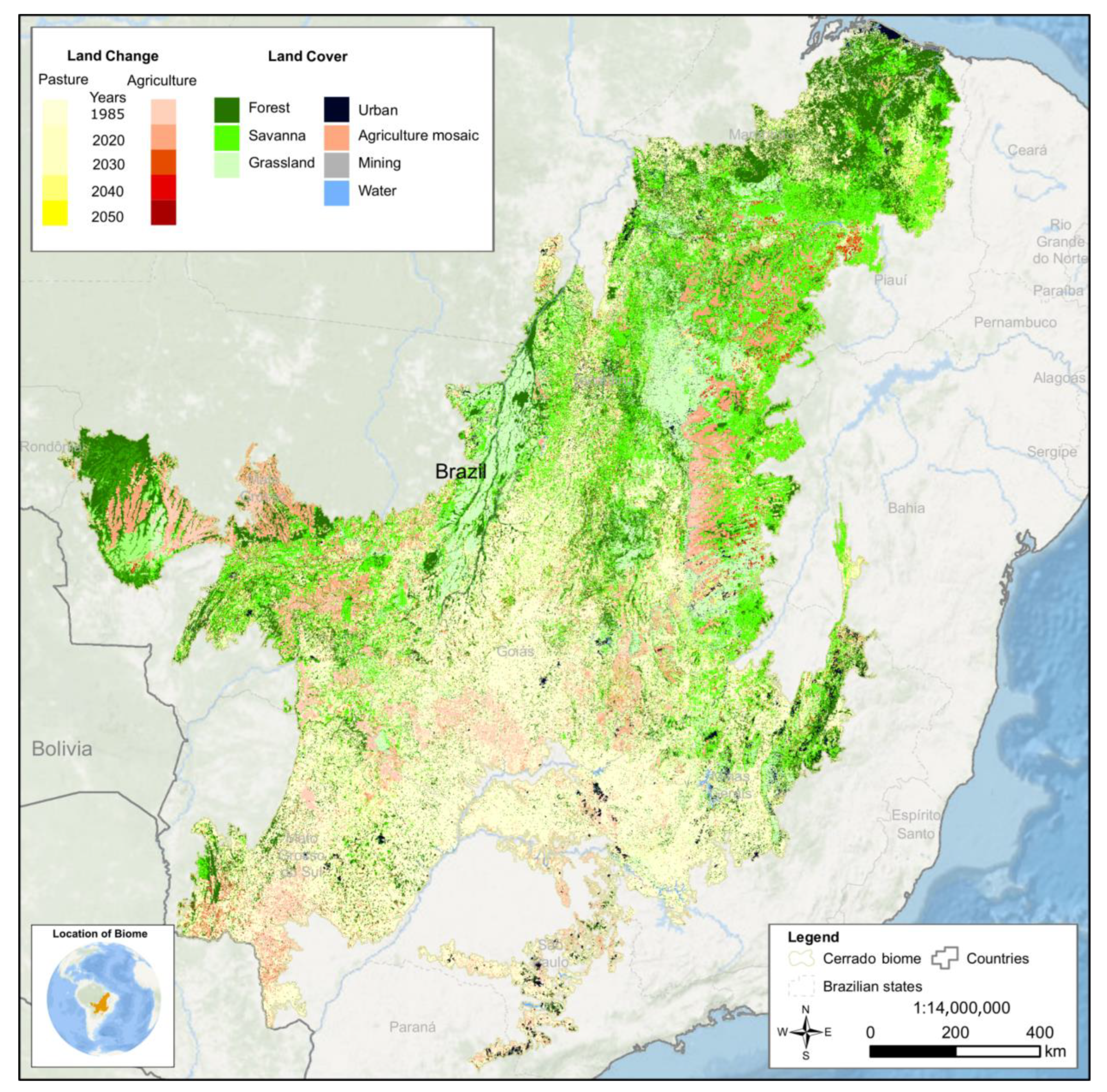
| Deforestation distance (natural log) | 0.38 | 0.89 | 0.72 | 0.53 | 0.48 | 0.47 | 0.17 | 0.1 | 0.06 | 0.08 | 0.07 | 0.007 |
| Friction (travel cost) | 0.26 | 0.63 | 0.3 | 0.37 | 0.35 | 0.34 | 0.14 | 0.36 | 0.06 | 0.01 | 0.03 | 0.001 |
| Slope | 0.28 | 0.87 | 0.49 | 0.41 | 0.37 | 0.33 | 0.12 | 0.1 | 0.06 | 0.05 | 0.04 | 0.006 |
| Altimetry | 0.28 | 0.87 | 0.49 | 0.42 | 0.36 | 0.33 | 0.14 | 0.07 | 0.06 | 0.05 | 0.04 | 0.006 |
| Rainfall of the rainiest month | 0.28 | 0.87 | 0.5 | 0.43 | 0.31 | 0.34 | 0.14 | 0.07 | 0.06 | 0.05 | 0.06 | 0.007 |
| Rainfall of the driest month | 0.24 | 0.67 | 0.51 | 0.25 | 0.3 | 0.18 | 0.16 | 0.05 | 0.04 | 0.05 | 0.11 | 0 |
| Soils | 0.27 | 0.87 | 0.48 | 0.48 | 0.3 | 0.33 | 0.11 | 0.06 | 0.06 | 0.05 | 0.04 | 0.005 |
| Soils (evidence likelihood) | 0.27 | 0.77 | 0.46 | 0.42 | 0.34 | 0.35 | 0.23 | 0.09 | 0.08 | 0.06 | 0.05 | 0.007 |
| Protected areas (natural log) | 0.29 | 0.87 | 0.51 | 0.41 | 0.31 | 0.4 | 0.11 | 0.07 | 0.08 | 0.06 | 0.06 | 0.005 |
| Legal reserves (natural Log) | 0.26 | 0.8 | 0.48 | 0.33 | 0.31 | 0.29 | 0.11 | 0.08 | 0.06 | 0.07 | 0.04 | 0.006 |
| Permanent preservation area (square root distance) | 0.28 | 0.85 | 0.49 | 0.4 | 0.31 | 0.34 | 0.11 | 0.06 | 0.06 | 0.05 | 0.07 | 0.006 |
| Valley (square root distance) | 0.11 | 0.59 | 0.32 | 0.27 | 0.32 | 0.19 | 0.1 | 0.1 | 0.04 | 0.04 | 0.02 | 0.003 |
| Hydrography (distance) | 0.05 | 0.01 | 0.003 | 0.0004 | 0.006 | 0.0019 | 0.001 | 0.07 | 0.14 | 0.02 | 0.0004 | |
| Limite constrange | 29 | 0.87 | 0.51 | 0.41 | 0.37 | 0.32 | 0.12 | 0.07 | 0.06 | 0.05 | 0.001 | 0.07 |
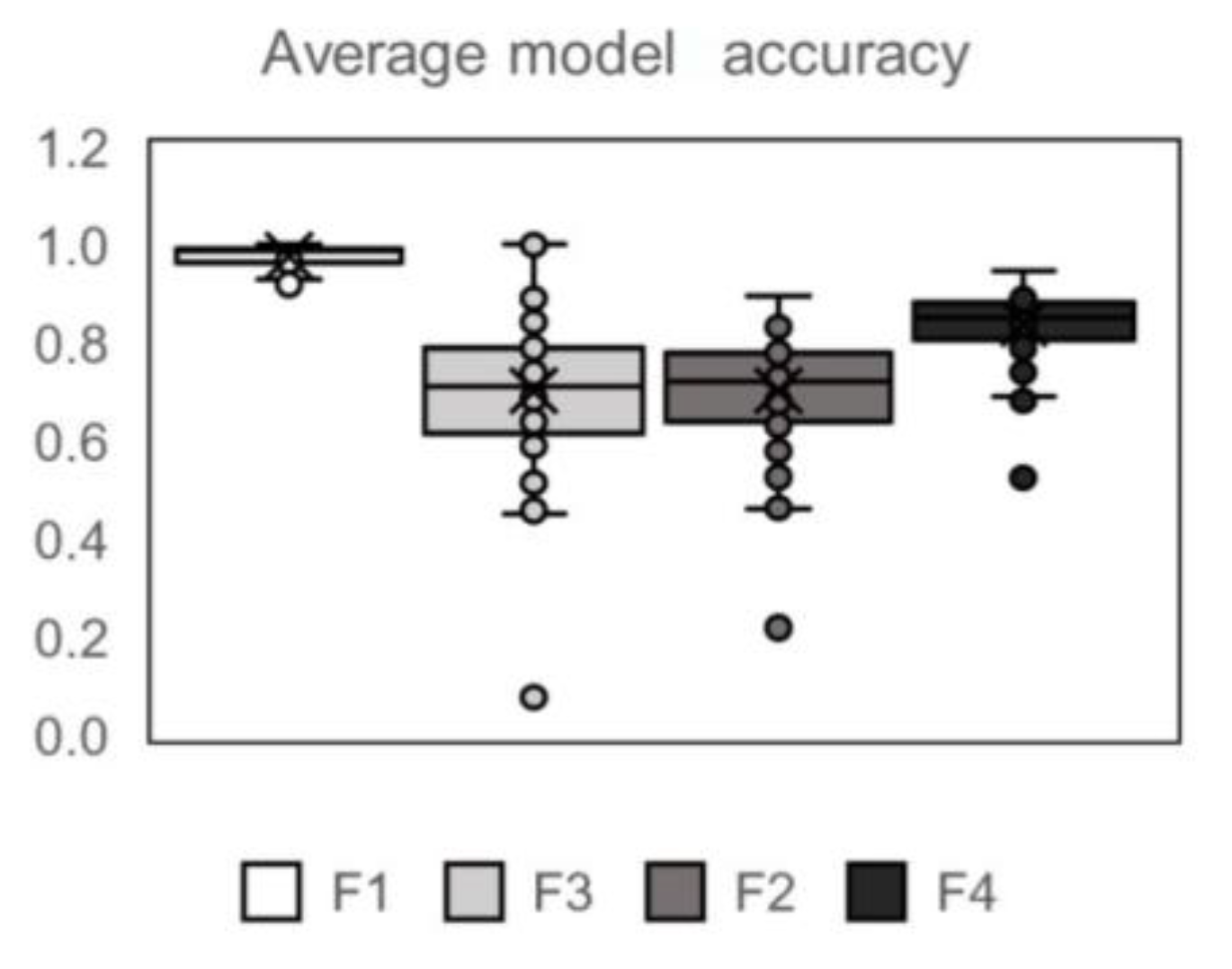
| Accuracy of Land Use Transitions | Model Accuracy | |||||
|---|---|---|---|---|---|---|
| Transition | Accuracy | Transition | Accuracy | Overall Model Accuracy Metrics | Model | Null Model |
| Forest to Pasture | 71.82% | Grassland to Mining | 77.78% | |||
| Forest to agriculture | 71.82% | Others to savanna | 67.51% | P(N) | 0.30 | 0.30 |
| Savanna to pasture | 75.20% | Others to grassland | 68.00% | P(M) | 0.99 | 0.99 |
| Savanna to silviculture | 83.25% | Others to pasture | 65.60% | P(P) | 1.00 | 1.00 |
| Savanna to mosaic | 88.98% | Others to agriculture | 76.38% | M(n) | 0.30 | 0.28 |
| Savanna to urban | 89.62% | Others to mosaic | 100% | M(m) | 0.99 | 0.96 |
| Savanna to agriculture | 73.65% | Pasture to grassland | 63.50% | M(p) | 0.99 | 0.96 |
| Grassland to pasture | 78.50% | Pasture to agriculture | 57.54% | N(n) | 0.09 | 0.09 |
| Grassland to agriculture | 80.04% | Pasture to mosaic | 77.00% | N(m) | 0.63 | 0.63 |
| Grassland to silviculture | 86.69% | Forest to silviculture | 98.04% | N(p) | 0.63 | 0.63 |
| Grassland to mosaic | 88.89% | Forest to mosaic | 98.44% | Kno | 0.99 | 0.96 |
| Grassland to urban | 92.45% | Savanna to forest | 61.01% | Klocation | 0.99 | 0.90 |
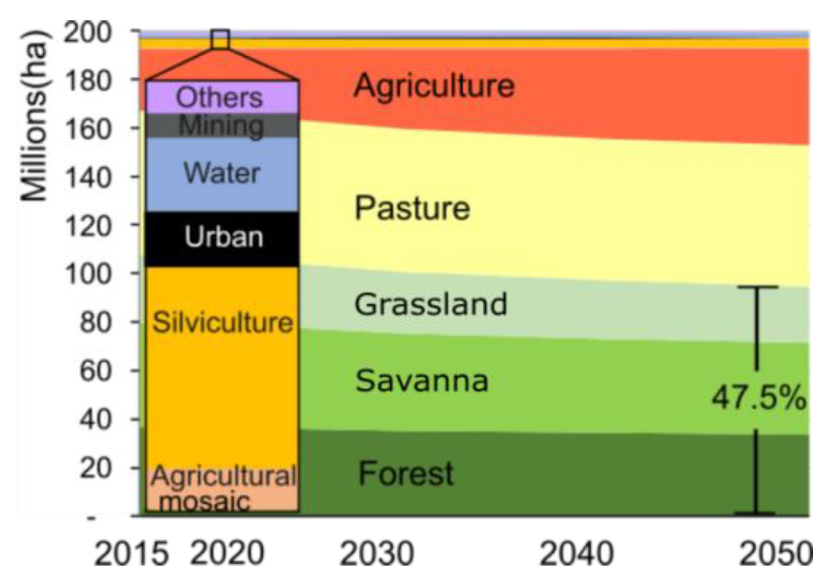
| Land Use | 2015 | 2018 | 2020 | 2030 | 2040 | 2050 |
|---|---|---|---|---|---|---|
| Forest | 18.40% | 18.70% | 18.50% | 17.70% | 17.20% | 16.90% |
| Savanna | 22.00% | 21.50% | 21.30% | 20.10% | 19.40% | 18.90% |
| Grassland | 14.40% | 14.10% | 13.90% | 12.80% | 12.20% | 11.70% |
| Others | 0.50% | 0.50% | 0.50% | 0.40% | 0.40% | 0.30% |
| Pastures | 30.00% | 30.00% | 29.80% | 29.40% | 29.20% | 29.10% |
| Agriculture | 11.70% | 12.20% | 13.00% | 16.60% | 18.60% | 20.00% |
| Silviculture | 1.70% | 1.70% | 1.70% | 1.70% | 1.70% | 1.70% |
| Agricultural mosaic | 0.30% | 0.30% | 0.30% | 0.30% | 0.30% | 0.30% |
| Urban areas | 0.30% | 0.40% | 0.40% | 0.40% | 0.40% | 0.40% |
| Mining | 0.00% | 0.00% | 0.00% | 0.00% | 0.00% | 0.00% |
| Water areas | 0.70% | 0.60% | 0.60% | 0.60% | 0.60% | 0.60% |
| Deforestation(km2) | 10.635 | 11.747 | 63.952 | 34.108 | 25.581 | |
| Deforestation(km2/year) | 3.545 | 5.874 | 6.395 | 3.411 | 2.558 | |
| Native remaining | 54.80% | 54.30% | 53.70% | 50.50% | 48.80% | 47.50% |
Disclaimer/Publisher’s Note: The statements, opinions and data contained in all publications are solely those of the individual author(s) and contributor(s) and not of MDPI and/or the editor(s). MDPI and/or the editor(s) disclaim responsibility for any injury to people or property resulting from any ideas, methods, instructions or products referred to in the content. |
© 2023 by the authors. Licensee MDPI, Basel, Switzerland. This article is an open access article distributed under the terms and conditions of the Creative Commons Attribution (CC BY) license (https://creativecommons.org/licenses/by/4.0/).
Share and Cite
Salmona, Y.B.; Matricardi, E.A.T.; Skole, D.L.; Silva, J.F.A.; Coelho Filho, O.d.A.; Pedlowski, M.A.; Sampaio, J.M.; Castrillón, L.C.R.; Brandão, R.A.; Silva, A.L.d.; et al. A Worrying Future for River Flows in the Brazilian Cerrado Provoked by Land Use and Climate Changes. Sustainability 2023, 15, 4251. https://0-doi-org.brum.beds.ac.uk/10.3390/su15054251
Salmona YB, Matricardi EAT, Skole DL, Silva JFA, Coelho Filho OdA, Pedlowski MA, Sampaio JM, Castrillón LCR, Brandão RA, Silva ALd, et al. A Worrying Future for River Flows in the Brazilian Cerrado Provoked by Land Use and Climate Changes. Sustainability. 2023; 15(5):4251. https://0-doi-org.brum.beds.ac.uk/10.3390/su15054251
Chicago/Turabian StyleSalmona, Yuri Botelho, Eraldo Aparecido Trondoli Matricardi, David Lewis Skole, João Flávio Andrade Silva, Osmar de Araújo Coelho Filho, Marcos Antonio Pedlowski, James Matos Sampaio, Leidi Cahola Ramírez Castrillón, Reuber Albuquerque Brandão, Andréa Leme da Silva, and et al. 2023. "A Worrying Future for River Flows in the Brazilian Cerrado Provoked by Land Use and Climate Changes" Sustainability 15, no. 5: 4251. https://0-doi-org.brum.beds.ac.uk/10.3390/su15054251