Soil Erosion Status Prediction Using a Novel Random Forest Model Optimized by Random Search Method

Abstract

Soil erosion, the degradation of the earth’s surface through the removal of soil particles, occurs in three phases: dislocation, transport, and deposition. Factors such as soil type, assembly, infiltration, and land cover influence the velocity of soil erosion. Soil erosion can result in soil loss in some areas and soil deposition in others. In this paper, we proposed the Random Search-Random Forest (RS-RF) model, which combines random search optimization with the Random Forest algorithm, for soil erosion prediction. This model helps to better understand and predict soil erosion dynamics, supporting informed decisions for soil conservation and land management practices. This study utilized a dataset comprising 236 instances with 11 features. The target feature’s class label indicates erosion (1) or non-erosion (−1). To assess the effectiveness of the classification techniques employed, six evaluation metrics, including accuracy, Matthews Correlation Coefficient (MCC), F1-score, precision, recall, and Area Under the Receiver Operating Characteristic Curve (AUC), were computed. The experimental findings illustrated that the RS-RF model achieved the best outcomes when compared with other machine learning techniques and previous studies using the same dataset with an accuracy rate of 97.4%.

1. Introduction

Soil erosion is the separation and wind-borne transportation of soil particles, water or other agents [1]. It is a natural process but can be accelerated by human activities such as deforestation, overgrazing, and inappropriate agricultural practices [2]. Unsustainable land use practices can lead to multiple negative impacts, including reduction in soil fertility and productivity, soil degradation and desertification, water pollution, loss of biodiversity and habitat, increased risk of natural disasters, and negative impacts on food security and human health. It is important to implement sustainable land management practices to mitigate these adverse effects and ensure a healthy and sustainable environment for current and future generations [3,4,5].

Reduction in soil fertility and productivity can occur due to various factors, including overuse of chemical fertilizers, erosion, and depletion of essential nutrients. Soil degradation and desertification, which are caused by activities such as deforestation, unsustainable agricultural practices, and mining, can result in the loss of fertile topsoil and the conversion of land into unproductive deserts [6].

Water pollution due to increased sedimentation can result from activities such as deforestation and land clearance, as sediment runoff can enter rivers and streams, negatively affecting water quality and aquatic ecosystems. This can have detrimental effects on marine life and other organisms dependent on clean water sources [7].

Loss of biodiversity and habitats for plants and animals can result from activities such as deforestation, land conversion, and habitat destruction. This can lead to the displacement and extinction of species, disrupting ecosystems and impacting the overall balance of ecosystems [8].

The increased risk of natural disasters such as landslides and flash floods can occur as a result of activities such as deforestation and improper land use. The removal of vegetation and disruption of natural drainage systems can exacerbate soil erosion and instability, leading to higher risks of landslides and flash floods, posing threats to human settlements and infrastructure [4,9].

Negative impacts on food security and human health can result from activities that degrade soil and water quality. This can affect agricultural productivity, crop yields, and access to clean water, leading to food shortages, malnutrition, and health issues for local communities who rely on agriculture for their livelihoods and sustenance [10].

Erosion can occur on various scales, from small-scale rills and gullies to large-scale land degradation [11,12].

In regions with abundant precipitation, erosion can be a significant concern, resulting in the gradual formation of deep gorges and canyons. However, there are several effective techniques available to mitigate soil erosion. These methods include the use of cover crops and conservation tillage to safeguard the soil surface, terracing to decelerate water flow and minimize erosion, vegetation planting to stabilize the soil and prevent erosion, as well as the construction of contour barriers and check dams to impede water flow and erosion. Additionally, implementing sustainable land use practices such as agroforestry and rotational grazing can also contribute to erosion control efforts [13].

It is important to address soil erosion as it has significant impacts on the environment, economy, and society. In order to preserve our natural resources and ensure food security, it is crucial to implement effective soil conservation measures [14]. Erosion is both a creative and destructive process in nature [15]. Benefits of erosion include the formation of alluvial plains, energy fields, rejuvenation of rivers, and the creation of soil. It also helps fight global warming, creates new habitats, binds carbon, and cleanses sites. However, excessive erosion can have negative impacts such as removing fertile soil and carrying agricultural chemicals into waterways. Erosion is a complex process in nature that involves both positive and negative outcomes. The formation of alluvial plains, energy fields, rejuvenated rivers, and soil are some of the benefits of erosion. It also helps mitigate global warming by removing carbon from the atmosphere and storing it in wetland areas. Erosion creates new habitats, binds carbon, and cleanses sites, but excessive erosion can lead to the loss of fertile soil and contamination of waterways with agricultural chemicals. Erosion is often viewed as a negative process, but it can also have positive impacts in nature. It helps to create alluvial plains, form energy sources such as coal and shale gas fields, rejuvenate rivers, and improve scenery and tourism. Additionally, soil erosion helps to fight global warming, create new soil and habitats, bind carbon, and cleanse the environment by diluting toxins in the ocean. Erosion is an ongoing process that weathers away rock into smaller particles that eventually form soil and create new habitats for life. The movement of soil and rock also helps to absorb carbon and remove it from the atmosphere [16].

Soil erosion can be studied using machine learning techniques for classification purposes. The major contribution of the study includes the training of a machine learning algorithm on a dataset of soil erosion patterns and characteristics, allowing the algorithm to classify new instances of soil erosion into predefined categories based on their similarity to the examples in the training dataset. This classification approach can aid in identifying different types of soil erosion and predicting their impacts on the environment. The study utilizes a soil erosion prediction classification model called Random Search-Random Forest (RS-RF). RS-RF is a machine learning model that combines two popular algorithms: Random Search and Random Forest. Random Search is an optimization algorithm used to identify the best set of hyperparameters for a given machine learning model. In contrast, Random Forest is an ensemble learning technique that integrates multiple decision trees for making predictions. RS-RF employs the Random Search algorithm to enhance the hyperparameters of the Random Forest algorithm, improving the accuracy of predictions. RS-RF is commonly used for classification and regression problems in various domains, including soil erosion prediction. The hypothesis of this study stated that the Random Search-Random Forest (RS-RF) model, trained on a dataset of soil erosion patterns and characteristics, will achieve higher accuracy in predicting soil erosion compared to other machine learning techniques, based on evaluation metrics such as accuracy, Matthews Correlation Coefficient (MCC), F1-score, precision, recall, and Area Under the Receiver Operating Characteristic Curve (AUC).”

This hypothesis suggests that the RS-RF model will outperform other machine learning techniques in accurately predicting soil erosion by utilizing the combined power of Random Search optimization and Random Forest algorithm. The study aims to validate this hypothesis by comparing the performance of RS-RF with other techniques and evaluating the results using various evaluation metrics. The organization of this paper is as follows: Section 2 presents the related work, Section 3 introduces the materials and methodologies used in this study, Section 4 presents the results and discussions, and finally, Section 5 concludes the paper with future directions.

2. Related Work

The use of Machine Learning (ML) in the assessment of plot experiment data for soil erosion prediction has become increasingly popular in recent years. These models, based on machine learning, provide a valuable solution to the complex and multivariate aspects of soil science and geoscience [17,18,19,20,21,22,23,24]. In Ref. [1], the authors studied the process of erosion model development; it involves two main stages: the creation of a physical model prototype and model evaluation. Once the model code and parameter experiments are completed, the parameter estimation stage can begin, which consists of parameter identification and the development of parameter prediction equations or techniques. The second phase of model development includes sensitivity analysis, confidence limit analysis, and validation with data. The WEPP (Water Erosion Prediction Project) and ANN (Artificial Neural Network) models are commonly used in soil science and hydrology to simulate soil loss. The WEPP model is a process-based erosion model that estimates soil erosion and sediment yield caused by water erosion. It simulates various erosion processes, such as rainfall detachment, runoff transport, and sediment detachment and transport. The ANN model, on the other hand, is a machine learning-based approach that uses artificial neural networks to model complex relationships between input variables (such as rainfall, slope, soil type) and output variables (such as soil loss). ANN models can capture nonlinearities and interactions among variables, making them useful for predicting soil erosion in complex environments. Both WEPP and ANN models have been widely used in erosion modeling and have their respective strengths and limitations [25,26,27].

Another study in [26] used ANN to estimate soil erosion and found that the amount of erosion was positively related to rainfall and runoff. In a study used in [27], WEPP and ANN models were used to simulate soil loss. The results showed that WEPP underpredicted soil loss, while the ANN outcomes were more in line with the observed data. In [28], the authors used ANN to forecast soil erodibility in Malaysia. In another study [29], used Kohonen neural networks (KNNs) for runoff-erosion modeling and found that KNNs outperformed the traditional multiple linear regression model.

In Ref. [30], the authors conducted to predict soil erosion in the Semenyih watershed in Malaysia by incorporating land cover dynamics using the LTM (Land Transformation Model) and USLE (Universal Soil Loss Equation) models. The research aimed to assess the impact of land cover changes on soil erosion potential in the watershed using these modeling approaches.

In Ref. [31], the authors used ANN to analyze erosion in a watershed and obtained good modeling outcomes. However, ANN has been heavily utilized in prior studies for analysis of erosion and these techniques are often trained with the steepest gradient descent and error backpropagation, which can result in getting trapped in locally optimal solutions [32,33,34,35]. Additionally, ANN is based on empirical risk minimization and can lead to overfitting [36]. A review of the literature suggests that more enhanced ML models may improve the modeling of soil erosion solutions and further investigation of other advanced algorithms is needed due to the complexity and dynamic nature of soil erosion prediction. The authors in Ref. [37] conducted a survey where they proposed a study for predicting soil erosion susceptibility using the Multivariate Adaptive Regression Splines (MARS) technique and Social Spider Algorithm (SSA) metaheuristic. The MARS model was used to construct a boundary that divided the input data into non-erosion and erosion zones, and the SSA metaheuristic was employed to optimize the effectiveness of MARS by tuning its hyperparameters. The combined method, called SSAO-MARS, was trained and tested using 236 soil plot conditions and corresponding erosion levels. The results showed a high classification accuracy rate of 96%, indicating that SSAO-MARS could be an effective tool for land management organizations. Additionally, the study utilized the Random Search-Random Forest (RS-RF) model for soil erosion forecasting, which was trained on a dataset with 11 features and 236 instances. Performance evaluation using various metrics showed that RS-RF outperformed other machine learning models and previous studies, achieving an accuracy rate of 97.4%. The utilization of ML approaches with optimizer and ensemble regression models may be helpful for achieving proposing results in both classification and regression issues [38,39,40,41,42,43].

3. Materials and Methods

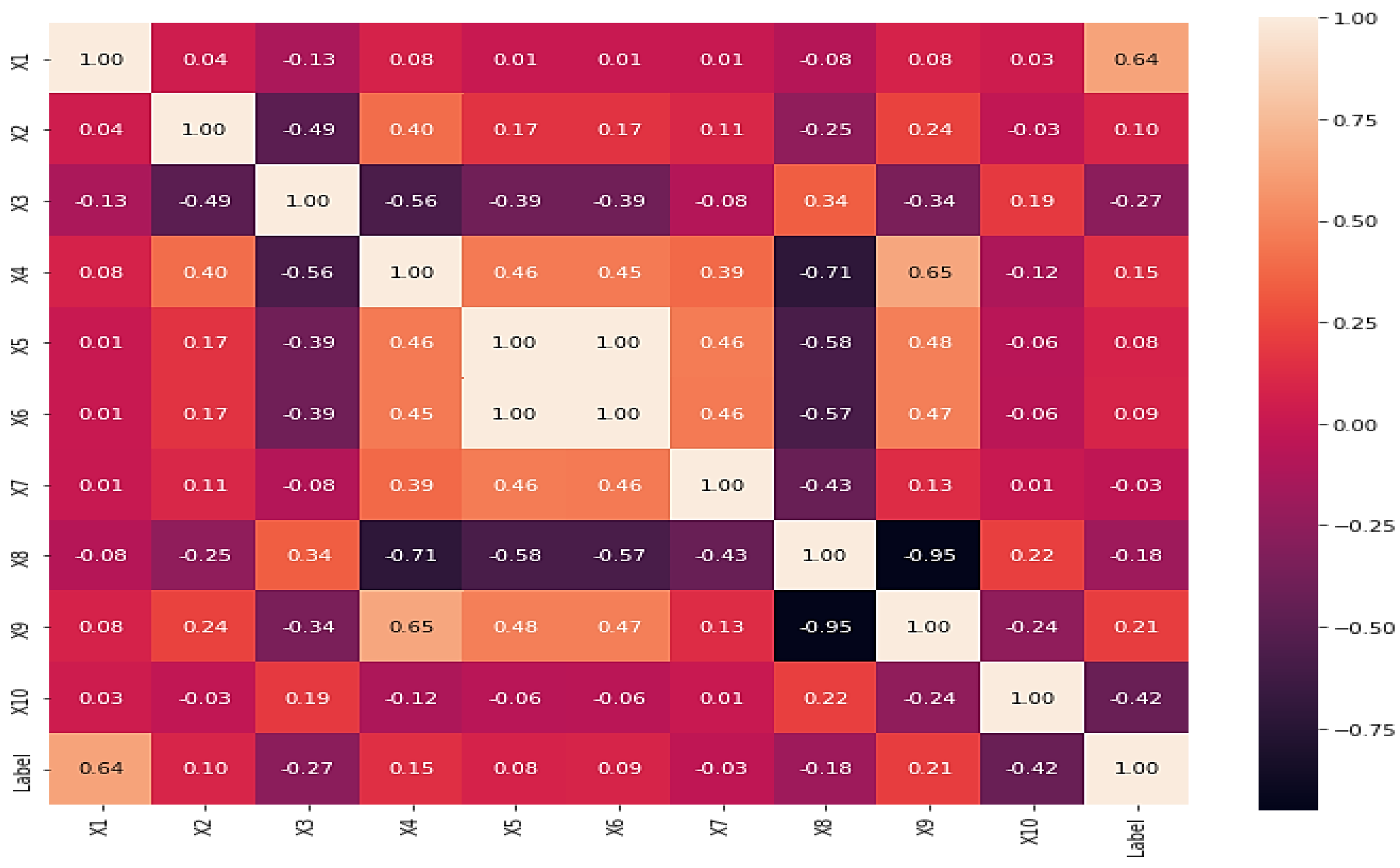
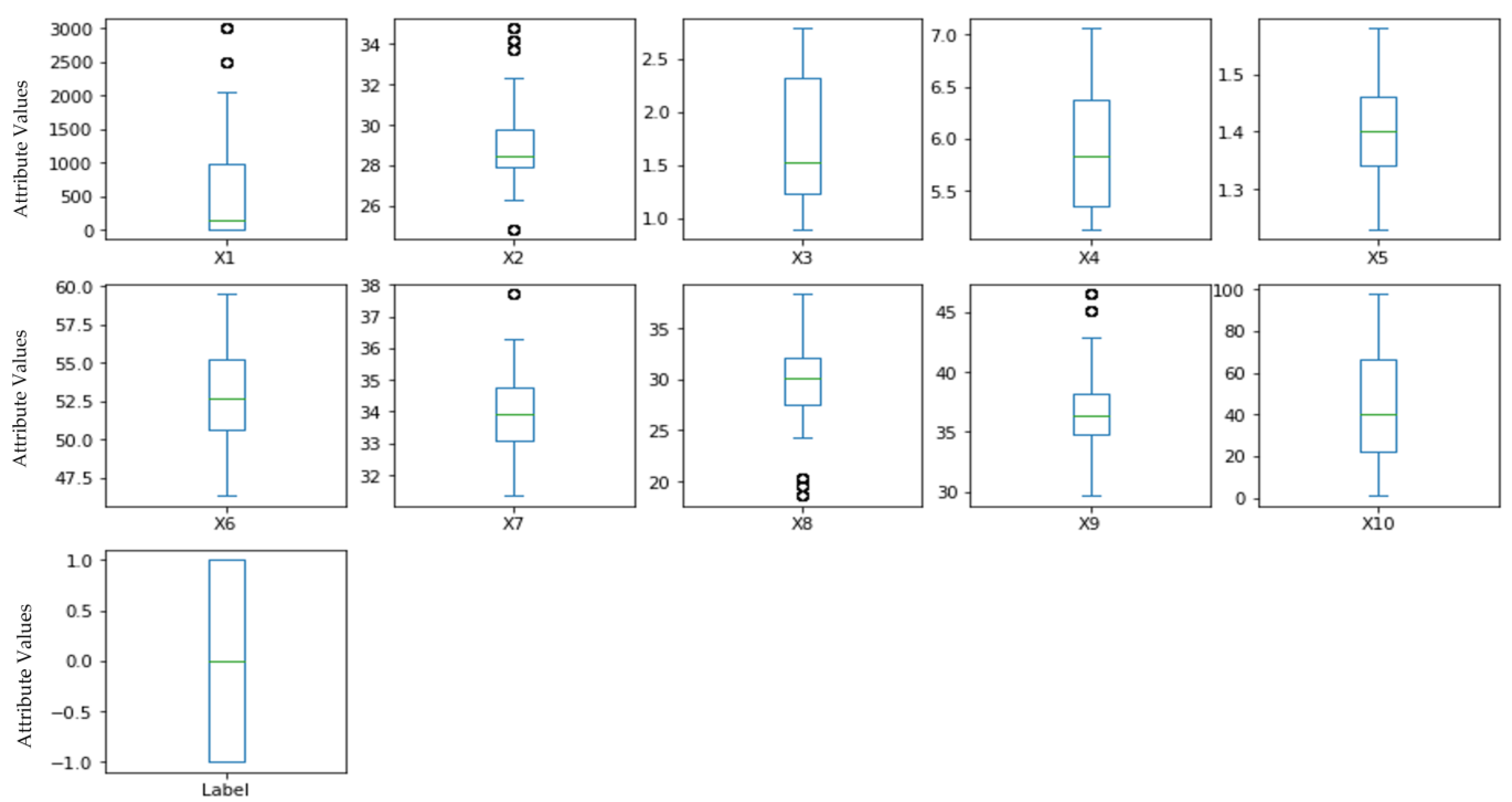
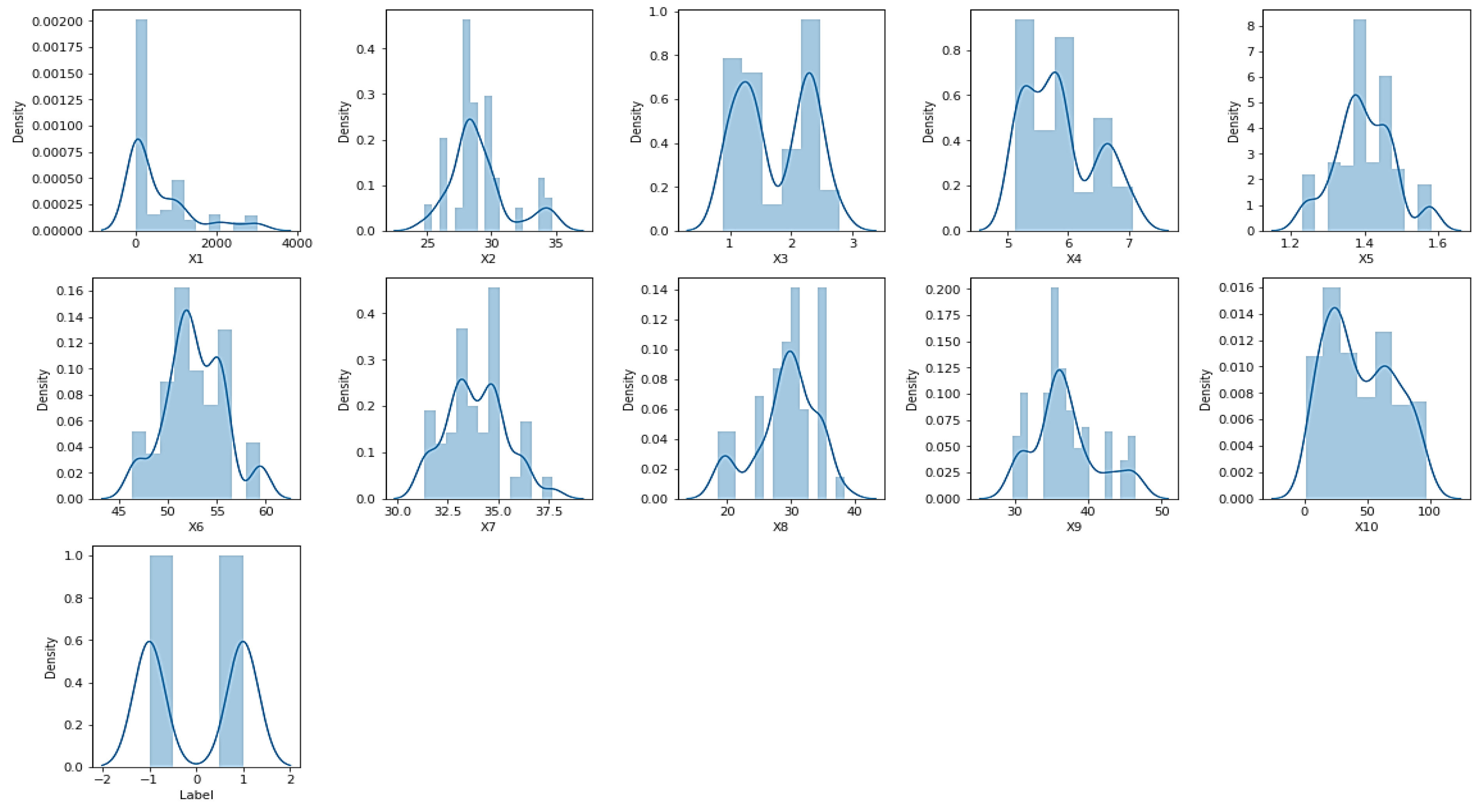
3.1. Dataset Description

In this paper, the dataset used is available at [37]. The data were collected over a three-year period (2009–2011) at two catchment areas in Vietnam’s northwest province of Son La. A tropical monsoon climate with a wet season from May to October and a dry, cold season from November to March characterizes the weather in both locations. The yearly average temperature is 21 °C, with February being 16 °C and August being 27 °C. The erosion plots, each measuring 4 m × 18 m and covering an area of 72 m², were set up to prevent water runoff from flowing outside. There was a total of 24 plots at both sites. At the base of each plot, a 200-L plastic tank was positioned with 16 outlet tubes spaced evenly along its top to monitor surface runoff. Clay loam to clay are the textures of the soils in the research locations, which are categorized as Alisols, Luvisols, or Calcisols. A randomized full-block design with four treatments and three replications was used to set up the experimental plots. The plots were typical USLE runoff plots, measuring 4 m in width and 18 m in slope. Slash-and-burn farming, fertilization-assisted plowing, soil conservation techniques such as grass barriers, cover crops, minimal tillage, and relay cropping with adzuki beans, were all used in the treatments as a traditional local maize farming practice. At each site, a bucket system was set up to collect sediment from soil erosion in the plots during the period from 2009 to 2011. This study used ten explanatory attributes to predict soil erosion, based on the available data. The attributes include slope, EI30, pH topsoil, organic carbon topsoil, total pore volume, bulk density, soil texture-clay, soil texture-silk, soil cover rate, and soil texture-sand. In this paper, we present the descriptive statistics of various attributes in

Table 1. Statistical description for the attributes.

Attributes	Notation	Count	Mean	Std	Min	50%	Max
EI30	X1	236	573.64	814.70	0	144.72	3008.93
Slope (degree)	X2	236	29.05	2.32	24.83	28.47	34.77
Organic carbon top soil (%)	X3	236	1.75	0.58	0.89	1.53	2.79
pH top soil	X4	236	5.87	0.58	5.13	5.83	7.06
Bulk density (g/cm3)	X5	236	1.40	0.08	1.23	1.40	1.58
Total pore volume (%)	X6	236	52.76	3.02	46.34	52.69	59.48
Soil texture-silk (%)	X7	236	33.90	1.49	31.35	33.93	37.71
Soil texture-clay (%)	X8	236	29.14	4.81	18.61	30.15	38.35
Soil texture-sand (%)	X9	236	36.95	4.38	29.66	36.37	46.51
Soil cover rate (%)	X10	236	44.28	26.74	1.05	40.42	97.64
Label	Label	236	0	1	−1	0	1

. Table 1 likely includes summary measures, such as measures of central tendency (e.g., count, mean, max, min), and measures of dispersion, e.g., the standard deviation for each attribute to summarize and describe the main characteristics of a dataset, providing a quantitative overview of the data.

Additionally, we provide a heatmap matrix in Figure 1 to visually represent the attributes. The heatmap matrix likely displays the relationships or patterns among the attributes in a tabular format, where rows and columns represent different attributes, and the cells are filled with colors that represent the strength or magnitude of the relationship between pairs of attributes. Heatmap matrices are commonly used in data visualization to explore and identify patterns, trends, or correlations among variables in a dataset. Figure 2 demonstrates a box plot for the distribution analysis of the features. Figure 3 demonstrates the histogram for the distribution analysis of the features.

3.2. Machine Learning Models

3.2.1. Random Forest (RF) Model

Random Forests is an ensemble technique that constructs numerous decision trees and combines them to generate a more accurate classifier. The decision tree algorithm employs entropy and information gain to identify the most discriminant characteristic for branching and to utilize it as the branching point. The RF classifier can reduce overfitting if the tree is sufficiently deep or if there are sufficient trees [44,45]. It is recognized as a valuable tool for regression and classification problems. Each decision tree functions as a voter, drawing inspiration from elections. The collection of votes for the final choice is utilized to increase the accuracy of forecasts [46]. Entropy and information gain are computed in accordance with Equations (1)–(3).

Gain(s,f) = E(s) − E(s,f)

(1)

$$\mathrm{E}(\mathrm{s})={\sum }_{i=1}^c-P_i{\log }_2{P}_i$$

(2)

$$\mathrm{E}(\mathrm{s},\mathrm{f})={\sum }_{c\in x}p\left(c\right)E\left(c\right)$$

(3)

where E(s) denoted the entropy of 2 classes, and E(s,f) represents the entropy of feature f. Algorithm 1 displays the pseudocode for the random forest method.

Algorithm 1 Pseudocode of RF Algorithm

To construct Ti, randomly sample the training data T using replacement. Generate a root node Ni, that contains containing Ti If N >1,    Pick x% at random from the potential dividing features in N.    Determine the information gain using Equation (1).    Choose the feature F that has the most information gain value.    Generate f child nodes of N, N1,…,Nf, where F has f potential values (F1,….,Ff)    For i from 1 to f do      Put the contents of Ni to Ti, as Ti contains all instances that match Fi in N      Repeat steps 3 through 9 for N times to create a forest of N trees.   End for End if

3.2.2. Naïve Bayes (NB) Model

As a simple probabilistic classification technique, the Naive Bayes (NB) algorithm obtains its probability value from the frequency computation and value associations from the connected material. In order to identify the class of the data that has to be evaluated, the NB classification process requires many guidelines or directives [47]. Therefore, Equation (4) is applied.

$$\mathrm{P}\left(\mathrm{c}|{\mathrm{F}}_1\dots .{\mathrm{F}}_{\mathrm{n}}\right)=\frac{\mathrm{P}\left(\mathrm{c}\right)\mathrm{P}({\mathrm{F}}_1\dots .{\mathrm{F}}_{\mathrm{n}}|\mathrm{c})}{\mathrm{P}({\mathrm{F}}_1\dots .{\mathrm{F}}_{\mathrm{n}})}$$

(4)

where $F_1\dots .F_n$ stands for features needed for categorization, and c denotes a class. Consequently, the probability of matching data with a certain feature in C class is C class probability emerged multiplied by the sample features probability in this class, and then divided by the samples features probability globally; posterior = [(class probability × likelihood)/evidence]. Algorithm 2 shows the pseudocode of the NB model.

Algorithm 2 Pseudocode of NB Model

Input: Training sample set N Output: A class of testing dataset. Check the training dataset N; Determine the standard deviation and mean of predictor parameter for each class; Repeat   Determine the fi probability in each class using the gauss density Equation (4); Until all predictor parameters probabilities (f1, f2, f3,..., fn) have been defined; Determine the samples features probability in each class; Obtain the largest probability.

3.2.3. Logistic Regression (LR) Model

The Logistic Regression Model, often known as the LR Model, is a common approach to modeling regression that takes into account both continuous and mixed independent variables as well as binary dependent variables [48]. The expression of logistic regression is denoted by the following Equation (5):

$$P=\frac{\text{exp}({\beta }_0+{\beta }_1{x}_{1+}\dots .+{\beta }_k{x}_k)}{1+\text{exp}({\beta }_0+{\beta }_1{x}_{1+}\dots .+{\beta }_k{x}_k)}$$

(5)

The success likelihood above the failure probability is determined by LR. The analysis’s outcomes are introduced as an odds ratio [49]. The logit transformation of Equation (6) was used to determine the regression coefficient.

$${\ln \left[\frac{p}{1-p}\right]=}_{\beta 0}+{\beta }_1{x}_{1+}{\beta }_2{x}_{2+}\dots .+{\beta }_k{x}_k$$

(6)

where p stands for the ecological land change probability, values range from 0–1, and 1 − p denotes the ecological land unchanged. Ln [p/(1 − p)] represents the log of the outputs, as the link function in generalized linear techniques. ${\beta }_0,{\beta }_1,{\beta }_2,\dots ,{\beta }_k$ are regression coefficients for the max likelihood method, and $x_1,x_2,\dots ,x_k$ are independent parameters.

3.2.4. K-Nearest Neighbor (KNN) Model

Although KNN was developed as a classification technique, it is now often utilized for non-parametric regression. The fundamental KNN algorithm calculating procedure may be stated as follows. In order to forecast the goal value, state vectors are built using present and historical data. Using the Euclidean distance that exists between the current state vector and each of the previous state vectors, the k historical moments that have the smallest distances are selected as the k-nearest neighbors. By determining the value that is, on average, held by k neighbors at the subsequent time point, the prediction outcome can be found for the target time [50].

3.2.5. Support Vector Machine (SVM) Model

Support Vector Machine, or SVM for short, is a method of ML that has gained a great deal of traction in recent years for its application in the analysis of neuroimaging data. Even in research projects with possibly limited data sets, SVMs stand out due to their exceptional capacity to deliver accurate performance predictions in a balanced manner. This is a result of the relative ease with which they can tackle a wide array of categorization issues as well as their adaptability [51,52]. Algorithm 3 shows the pseudocode of the SVM model.

Algorithm 3 Pseudocode of the SVM Model

Make the data set normalized, For Each C, γ: while C variable trades off the training instances misclassification against the decision surface simplicity, and γ parameter determines how much effect a single training example has. Use leave-one-out cross validation. a. Develop and evaluate the SVM. b. Save the achievement rate. Determine the average success rate. If necessary, update the best γ and C. With the next values of C, γ, return to step 3. Select γ, C with the highest average success rate, then carry out step 2 using a fine scale around the variables you’ve chosen.

3.2.6. Linear Discriminant Analysis (LDA) Model

The LDA method categorizes data into vector format using linear combinations of characteristics based on class variables or a target factor. It is a variation of Fisher’s linear discriminant. Five simple steps may be used to create the LDA algorithm [53]. When conducting LDA classification, the first step is to calculate the d-dimensional mean vectors for the classes found in the dataset by determining the mean (μ) of each given attribute (x) in each class (k), as shown in Equation (7).

$$\mu =\frac{1}{nk}\sum \left(x\right)$$

(7)

where n refers to the whole dataset’s observation number. Subsequently, a matrix representing the calculated within-class and between-class scatters is returned. Based on Equations (8) and (9) the within-class dispersion or distances are calculated.

$$S_{within}=\sum _{i=1}^c{S}_i$$

(8)

$$S_i=\sum _{x\in Di}^n(x-{\mu }_i){(x-{\mu }_i)}^T$$

(9)

where i represents the scatter for each class found in the dataset. The between-class scatter is computed using Equation (10).

$$S_{between}=\sum _{i-1}^c{N}_i({\mu }_i-\mu ){({\mu }_i-\mu )}^T$$

(10)

where $\mu$ signifies the sample mean of recognized classes, and N is the size of the classes that were found. In the third stage, Eigenvectors related to the product of the out-of-class and within-class matrices are solved. The linear discriminant is sorted in the fourth phase to find the new feature subspace utilizing diminishing Eigenvalue amplitudes to pick and sort. The observations or samples are changed into the new sub-spaces in the last phase.

3.2.7. Stochastic Gradient Descent (SGD) Model

By modifying the parameters that are adaptive to the stochastic gradient descent (SGD), the LR model may be constructed. The initial sample of data should be split into training sets and testing sets before the model creation process. The earlier set is used to change the model’s variables, while the second set is saved for verifying the technique’s generalization capabilities [54]. Algorithm 4 describes the SGD steps.

Algorithm 4 Pseudo-code for Stochastic Gradient Descent (SGD)

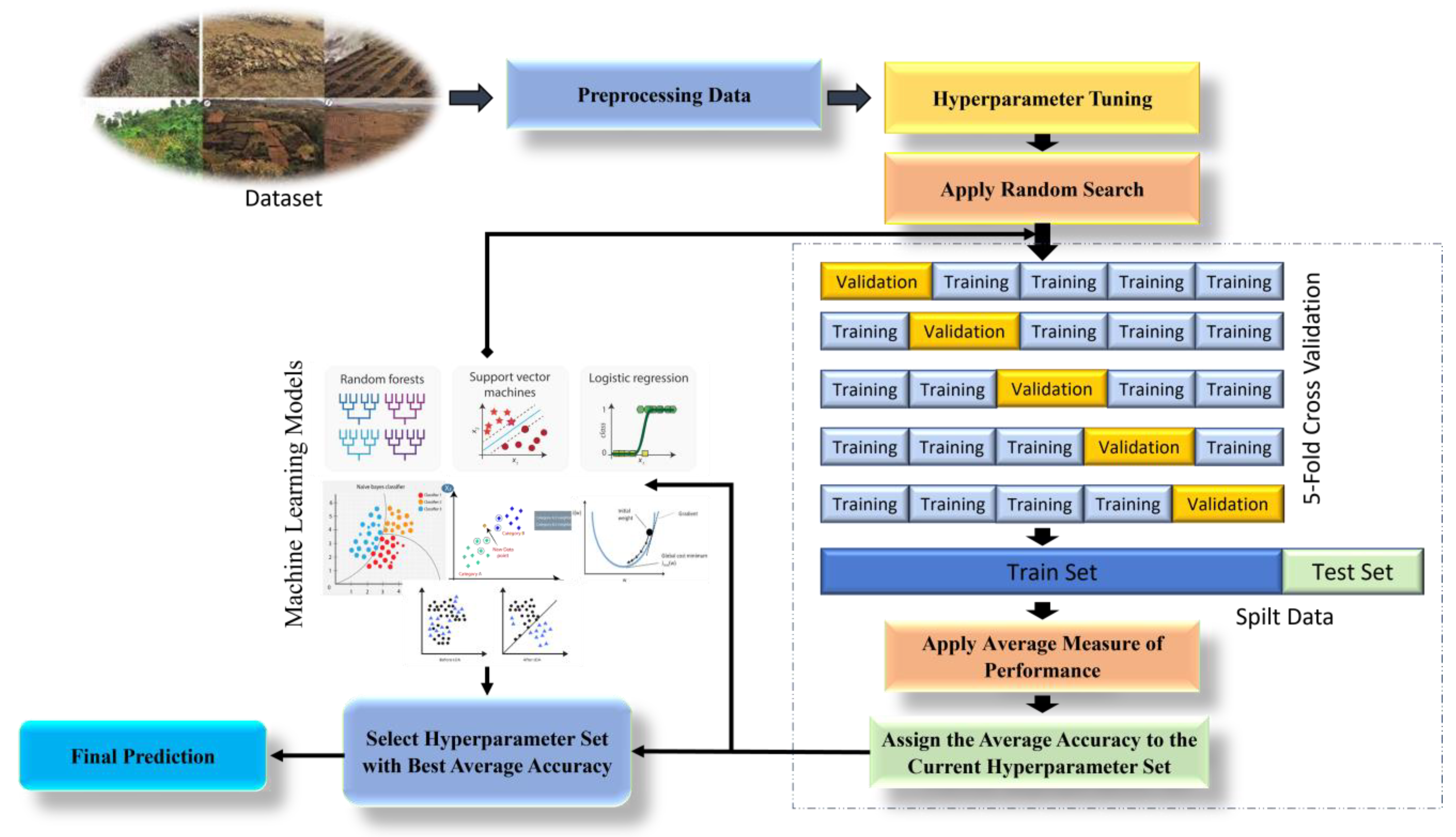
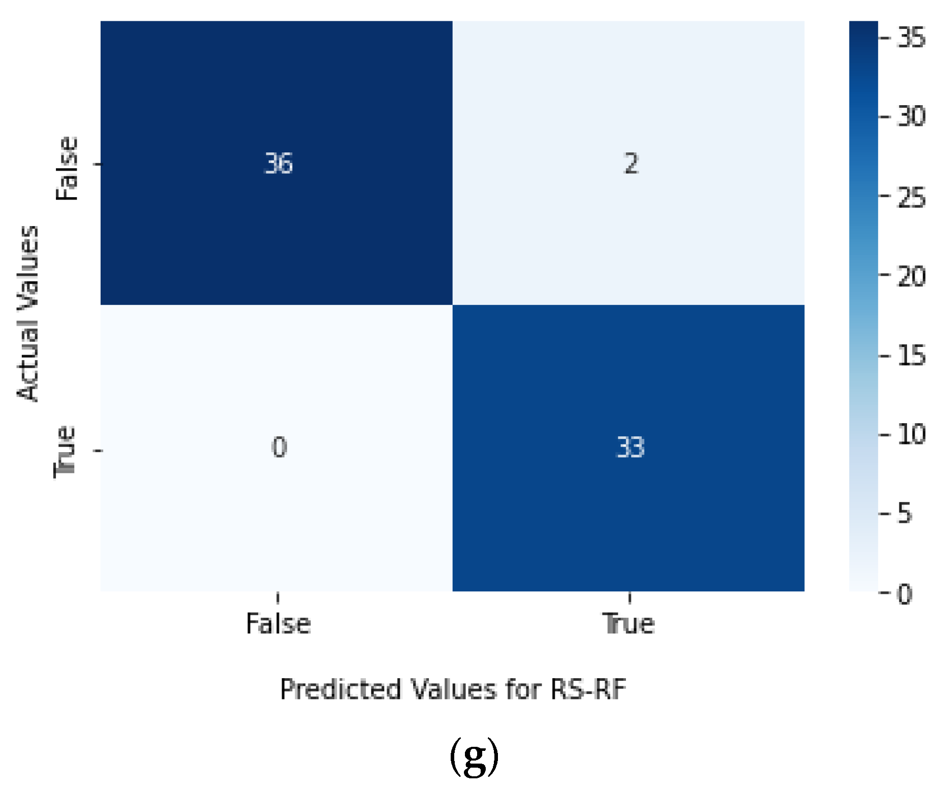
3.3. The Proposed RS-RF for Soil Erosion Status Prediction

This section explains how to combine the random search method with the random forest model to greatly enhance the generalization of decision thresholds for two classes of soil erosion data: erosion and non-erosion. In order to classify patterns, the following influencing parameters are used: slope, EI30, pH top soil, organic carbon top soil, total pore volume, bulk density, soil texture-clay, soil texture-silk, soil cover rate, and soil texture-sand. N-estmators (Ne) and Criterion (C) are two hyper-parameters of RF that are noteworthy. It is necessary for the RS to concurrently search these hyper-parameters. It should be mentioned that the proposed technique was developed using the built-in functionalities of Jupyter in a Python environment.

3.3.1. Data Normalization

The Min-Max equation is used in this research to adjust the values of the influencing elements to a standard limit. It is the simplest kind of normalization that aims to scale all variables to fall between [0, 1]. The value x_i is modified to a brand-new value in the range [0, 1] for each value in attribute A. Equation (12) represents the Min-max formula.

$$X_i=\frac{x_i-Min}{Max-Min}$$

(12)

The whole soil erosion dataset is then split into two sets. The first set, which made up 70% of the data pattern and is referred to as the training set, is used to build the non-erosion/erosion classification technique, and the second set, which made up the remaining 30% of the dataset and referred to the testing dataset, is used to verify the generalizability of the trained classification model. A cross-validation approach is used and equals 5 to generalize the classification findings and improve the system’s reliability. In this research, the suggested models Linear Discriminant Analysis (LDA), Stochastic Gradient Descent (SGD), K-Nearest Neighbor (KNN), Support Vector Machine (SVM), Logistic Regression (LR), Random Forest (RF), and Naive Bayes (NB) are compared to the proposed RS-RF model.

3.3.2. Random Search (RS)

Random search is the baseline scheduling approach; for an optimization strategy to be deemed feasible, it must outperform random searching for better solutions. Random Search is an example of a Monte Carlo method, as a very basic Monte Carlo strategy that uses no problem-specific information to merely assign management units to harvest time possibilities and serves as a search process guide at random [55]. The procedure involves randomly assigning a harvest time, including the option of a no-harvest prescription, to all management units. The wildlife objectives are then assessed, and if the resulting objective function is achievable and superior to the best solution found so far, it is stored as the optimal solution. This initial step is different from the subsequent seven processes, where only minor modifications are made to the solution during iterations. There may be additional methods to improve the Monte Carlo search process, but RS is utilized as a general mechanism, random chance, to evaluate the other strategies [56].

3.3.3. Proposed Methodology

Using the RS metaheuristic, this work seeks to maximize the performance of the RF model. As mentioned in the previous section, the RS starts with the random initialization of a set of hyper-parameters (e.g., c and Ne). With each subsequent generation, this metaheuristic method searches and utilizes the search space to find promising regions containing high-quality sets of the RF model’s hyperparameters. Using the hyper-parameters identified by the RS metaheuristic, the RF model evaluates the training set and generalizes a decision limit that splits input sequences related to erosion from those related to non-erosion classes. This research employed a K-fold cross-validation method with K = 5 to define the objective function of the RS. The dataset is separated into five mutually exclusive groups based on the cross-validation approach. In each of the five iterations, one set is utilized to verify the model, while the remaining four sets serve as training data. The mean forecast accuracy produced from five folds is used to measure the soil erosion forecasting model’s capacity to adapt. Consequently, the objective function for the RS metaheuristic is given by Equation (13):

$$F=\sum _{i=1}^5\left(\frac{\left(\frac{FN}{FN+TP}\right)+\left(\frac{FP}{FP+TN}\right)}{5}\right)$$

(13)

where TP, TN, FN, and FP represent the number of true positives, true negatives, false negatives, and false positives obtained from the ith run, respectively. The RS-RF model’s operating process is shown in Figure 4. Algorithm 5 displays the pseudocode of the proposed Random Search-Random Forest (RS-RF).

Algorithm 5 Pseudocode of the proposed Random Search-Random Forest (RS-RF)

Select randomly M features from total feature set Among M features:    Calculate information gain    Select node d which has the highest information gain    Spilt nodes into daughter nodes    Repeat steps from 1–5 until predefined number of nodes is reached Build forest by repeating step 6 to create number of trees Apply random search for each subtree For each iteration do   Takes test features   Calculate accuracy of each randomly created trees   Calculate averaging for all subtrees Return hyperparameter set with best average accuracy

3.4. Evaluation Metrics

In this paper, Accuracy, F1-score, Precision, Matthews Correlation Coefficient (MCC), Recall, and Area Under Curve (AUC) metrics were computed based on the confusion matrix. The formula for each measure is specified using Equations (14)–(19) [57].

$$\mathrm{Accuracy}=\frac{TN+TP}{TP+TN+FP+FN}\ast 100$$

(14)

$$\mathrm{Matthews}\mathrm{Correlation}\mathrm{Coefficient}(\mathrm{MCC})=\frac{\left(TP\ast TN\right)-(FN\ast FP)}{\sqrt{\left(TP+FN\right)\ast \left(TP+FP\right)\ast \left(TN+FP\right)\ast (TN+FN)}}$$

(15)

$$\mathrm{F}1\mathrm{-Score}=\frac{2TP}{2TP+FP+FN}$$

(16)

$$\mathrm{Recall}=\frac{TP}{TP+FN}$$

(17)

$$\mathrm{Precision}=\frac{TP}{TP+FP}$$

(18)

$$\mathrm{AUC}=\frac{1}{2}\left(\frac{TP}{TP+FN}+\frac{TN}{TN+FP}\right)$$

(19)

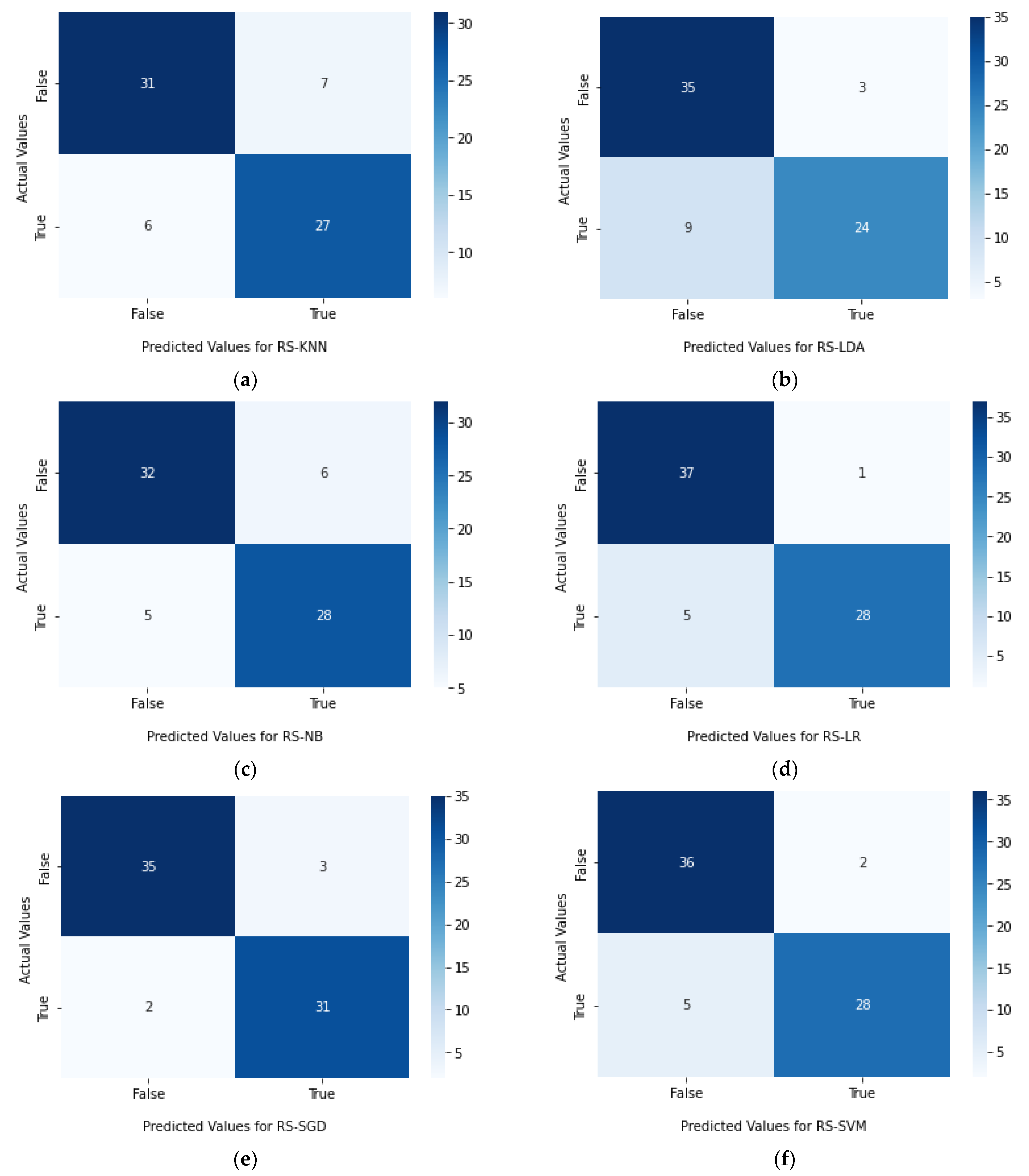
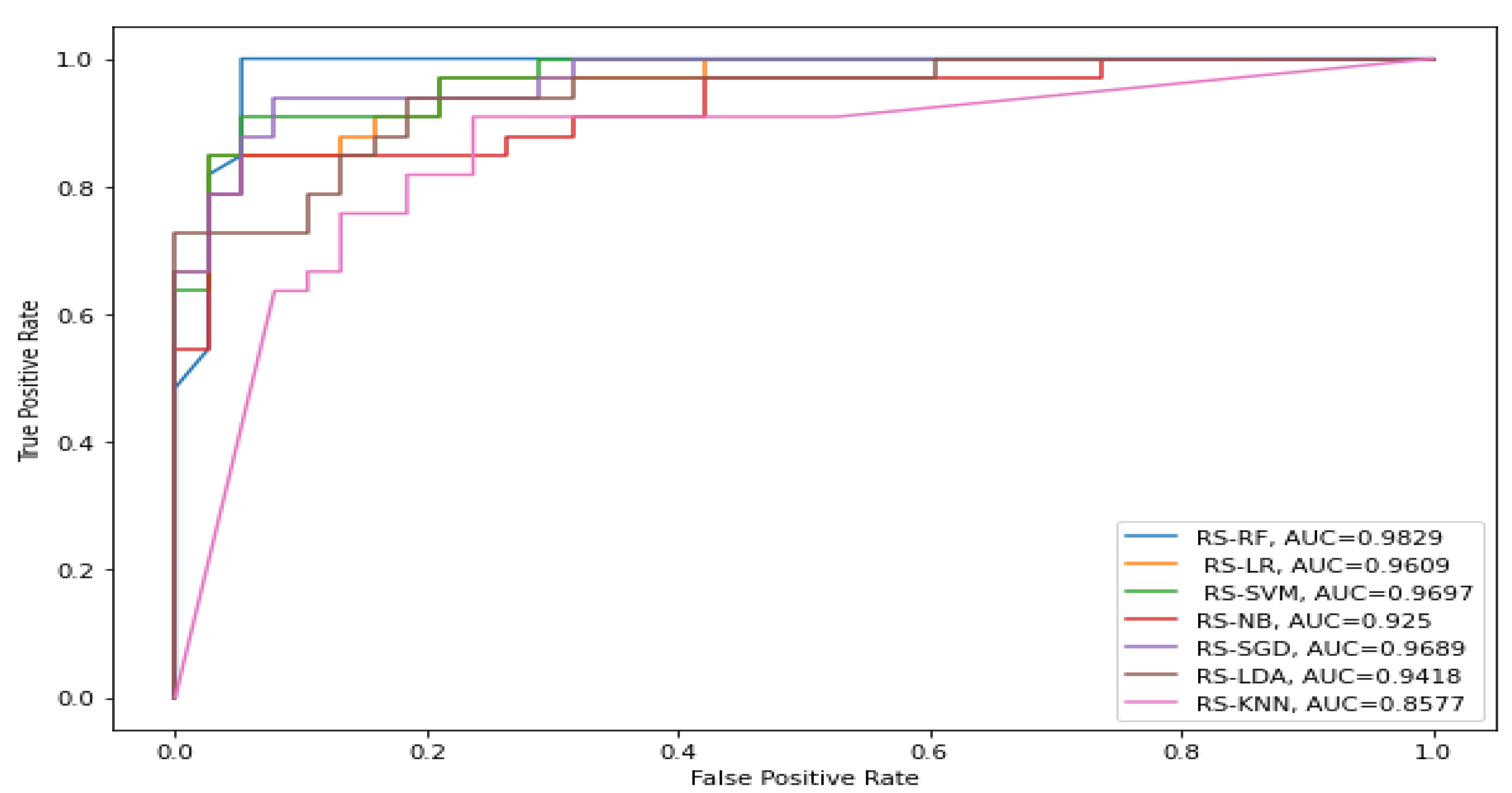
4. Results and Discussion

Jupiter notebook version (6.4.6) is used to perform the experimental findings. Jupiter notebook facilitates the execution and authoring of Python programs. It is extensively used as an open-source implementation and execution tool of artificial intelligence (AI) and machine learning models. The performance of the proposed technique is compared to several models. The performance of the classification models was evaluated using the evaluation metrics, namely, accuracy, MCC, F1 score, recall, precision, and AUC.

Table 2. Best parameters for the classification models using random search method.

Models	Tuning Parameters	Best Parameters
RF	N_estimators = [50, 100, 150, 200, 250], criterion = [‘gini’, ‘entropy’].	N_estimators = 150, criterion = gini.
KNN	N_neighbors = [5, 10, 15, 20, 25, 30], weights = [‘uniform’, ‘distance’].	N_neighbors = 15, weights = distance.
LDA	N_components = [1, 2, 3, 4, 5, 6, 7, 8, 9, 10].	N_components = 1.
NB	Alpha = [0.1, 0.2, 0.3, 0.4, 0.5, 0.6, 0.7, 0.8, 0.9, 1].	Alpha = 0.6.
LR	Penalty = [l1′, ‘l2′, ‘elasticnet’], solver = [‘lbfgs’, ‘liblinear’, ‘saga’].	Penalty = l2, solver = lbfgs.
SGD	Loss = [‘hinge’, ‘log_loss’, ‘log’], penalty = [l1′, ‘l2′, ‘elasticnet’].	Loss = log, penalty = l1.
SVM	Kernel = [‘linear’, ‘poly’, ‘rbf’, ‘sigmoid’], regularization parameter (C) = [0.1, 0.2, 0.3, 0.4].	Kernel = rbf, C = 0.2.

presents the best variables for the classification techniques using the RS method.

Figure 5 demonstrates the predicted and actual values for the models namely, RS-KNN, RS-LDA, RS-NB, RS-LR, RS-SGD, RS-SVM, and the proposed RS-RF. Furthermore, it shows the results obtained as confusion metrics for the proposed RS-RF compared with ML models in the testing phase. The Python code generated a figure showing the results of evaluating the metrics using a confusion matrix. The dataset was divided into a 70% training set and a 30% test set. Figure 5 displays the evaluation metrics for 71 attributes. The intensity of the blue color represents the values, with darker blue indicating higher values and brighter blue indicating lower values.

The AUC is calculated by plotting the Receiver Operating Characteristic (ROC) curve, which is a graphical representation of a model’s true positive rate (sensitivity) against its false positive rate (1-specificity) at different classification thresholds. The AUC represents the area under this curve, with a higher value indicating better model performance as shown in Figure 6. The AUC values for the models namely, RS-RF, RS-LR, RS-SVM, RS-NB, RS-SGD, RS-LDA, and RS-KNN. It can be seen that the AUC value of the RS-RF model is 0.9829, this value is good as it is near 1.

Table 3. Performance of the classification models.

Models	Accuracy	MCC	F1 Score	Recall	Precision	AUC
RS-KNN	81.60%	63.20%	81.70%	81.60%	81.70%	0.8577
RS-LDA	83.10%	66.60%	82.80%	83.10%	83.80%	0.9418
RS-NB	84.50%	68.90%	84.50%	84.50%	84.60%	0.925
RS-LR	91.50%	83.40%	91.40%	91.50%	92.00%	0.9609
RS-SGD	92.90%	85.90%	92.90%	92.90%	93.00%	0.9689
RS-SVM	90.10%	80.30%	90.10%	90.10%	90.30%	0.9697
RS-RF	97.40%	95.10%	97.30%	97.30%	97.50%	0.9829

displays the accuracy, MCC, F1 score, recall, precision, and AUC experimental results for the RS-KNN model, RS-LDA model, RS-NB model, RS-LR model, RS-SGD model, RS-SVM model, and RS-RF model, respectively. As seen in Table 3, the best outcomes of the assessment measures are printed in bold.

As shown in Table 3, the performance of the classification models using random search method, namely, the RS-KNN model, RS-LDA model, RS-NB model, RS-LR model, RS-SGD model, RS-SVM model, and RS-RF model are demonstrated. The proposed RS-RF model presents the best results than other classification models, namely, the RS-KNN model, RS-LDA model, RS-NB model, RS-LR model, RS-SGD model, and RS-SVM model. The proposed RS-RF model accuracy, MCC, F1 score, recall, precision, and AUC are 97.4%, 95.1%, 97.3%, 97.3%, 97.5% and 0.9829, respectively. The RS-KNN model performed the lowest, its accuracy, MCC, F1 score, recall, precision, and AUC are 81.6%, 63.2%, 81.7%, 81.6%, 81.7% and 0.8577, respectively. A comparison between the proposed RS-RF classification model using a random search method with a study using the same dataset is listed in

Table 4. Comparative study of this work with another study used the same dataset.

Studies	Model	Accuracy
Ref. [37]	SSAO-MARS	96.00%
Proposed RS-RF	Random search with random forest	97.40%

. From Table 4, the proposed RS-RF model achieved better performance in terms of accuracy than the previous study.

5. Conclusions and Future Work

In recent times, machine learning models and optimization methods have been increasingly used for soil erosion classification. In this study, we employed the random search (RS) optimization method to fine-tune the parameters of seven different classification models, namely, random forest (RF), logistic regression (LR), naïve Bayes (NB), support vector machine (SVM), stochastic gradient descent (SGD), K-Nearest Neighbor (KNN), and linear discriminant analysis (LDA), for predicting soil erosion. Six evaluation metrics, including MCC, accuracy, F1 score, recall, precision, and AUC, were utilized to assess the performance of these classification models. Our experimental results revealed that the proposed RS-RF approach, which combined the random search method with the random forest model, achieved the highest accuracy of 97.4% in predicting soil erosion. On the other hand, the RS-KNN model performed relatively less accurately with an accuracy of 81.6%.

In the future, there is potential for collecting larger datasets from diverse areas to further improve the accuracy of soil erosion prediction models. Additionally, exploring other machine learning techniques such as deep learning (DL) and statistical models could be beneficial in achieving even better results. Overall, this study contributes to the growing body of research on soil erosion prediction using machine learning and optimization techniques and opens avenues for future research in this field.

References

1. Nearing, M.A.; Lane, L.J.; Lopes, V.L. Modeling Soil Erosion. In Soil Erosion Research Methods; Routledge: Oxford, UK, 2017; pp. 127–158. ISBN 0-203-73935-3. [Google Scholar]
2. Batista, P.V.; Davies, J.; Silva, M.L.; Quinton, J.N. On the Evaluation of Soil Erosion Models: Are We Doing Enough? Earth-Sci. Rev. 2019, 197, 102898. [Google Scholar] [CrossRef]
3. Wang, J.; Zhen, J.; Hu, W.; Chen, S.; Lizaga, I.; Zeraatpisheh, M.; Yang, X. Remote Sensing of Soil Degradation: Progress and Perspective. Int. Soil Water Conserv. Res. 2023; in press. [Google Scholar] [CrossRef]
4. AbdelRahman, M.A. An Overview of Land Degradation, Desertification and Sustainable Land Management Using GIS and Remote Sensing Applications. Rend. Lincei. Sci. Fis. Nat. 2023, 1–42. [Google Scholar] [CrossRef]
5. Kryuchkov, S.N.; Solonkin, A.V.; Solomentseva, A.S.; Zholobova, O.O. Elements of the Technology of Reproduction of Robinia Pseudoacacia L. for Protective Afforestation under Conditions of Land Degradation and Desertification. Arid Ecosyst. 2023, 13, 83–91. [Google Scholar] [CrossRef]
6. Osman, K.T. Soil Degradation, Conservation and Remediation; Springer: Dordrecht, The Netherlands, 2014; Volume 820. [Google Scholar]
7. Nosair, A.M.; Shams, M.Y.; AbouElmagd, L.M.; Hassanein, A.E.; Fryar, A.E.; Abu Salem, H.S. Predictive Model for Progressive Salinization in a Coastal Aquifer Using Artificial Intelligence and Hydrogeochemical Techniques: A Case Study of the Nile Delta Aquifer, Egypt. Environ. Sci. Pollut. Res. 2022, 29, 9318–9340. [Google Scholar] [CrossRef]
8. Mills, S.C.; Socolar, J.B.; Edwards, F.A.; Parra, E.; Martínez-Revelo, D.E.; Ochoa Quintero, J.M.; Haugaasen, T.; Freckleton, R.P.; Barlow, J.; Edwards, D.P. High Sensitivity of Tropical Forest Birds to Deforestation at Lower Altitudes. Ecology 2023, 104, e3867. [Google Scholar] [CrossRef]
9. Tang, H.; Shi, P.; Fu, X. An Analysis of Soil Erosion on Construction Sites in Megacities Using Analytic Hierarchy Process. Sustainability 2023, 15, 1325. [Google Scholar] [CrossRef]
10. Mkhize, X.; Mthembu, B.E.; Napier, C. Transforming a Local Food System to Address Food and Nutrition Insecurity in an Urban Informal Settlement Area: A Study in Umlazi Township in Durban, South Africa. J. Agric. Food Res. 2023, 12, 100565. [Google Scholar] [CrossRef]
11. Pimentel, D. Soil Erosion: A Food and Environmental Threat. Environ. Dev. Sustain. 2006, 8, 119–137. [Google Scholar] [CrossRef]
12. Montgomery, D.R. Soil Erosion and Agricultural Sustainability. Proc. Natl. Acad. Sci. USA 2007, 104, 13268–13272. [Google Scholar] [CrossRef]
13. Chalise, D.; Kumar, L.; Kristiansen, P. Land Degradation by Soil Erosion in Nepal: A Review. Soil Syst. 2019, 3, 12. [Google Scholar] [CrossRef]
14. Toy, T.J.; Foster, G.R.; Renard, K.G. Soil Erosion: Processes, Prediction, Measurement, and Control; John Wiley & Sons: Hoboken, NJ, USA, 2002; ISBN 0-471-38369-4. [Google Scholar]
15. Lal, R.; Moldenhauer, W.C. Effects of Soil Erosion on Crop Productivity. Crit. Rev. Plant Sci. 1987, 5, 303–367. [Google Scholar] [CrossRef]
16. Pimentel, D.; Burgess, M. Soil Erosion Threatens Food Production. Agriculture 2013, 3, 443–463. [Google Scholar] [CrossRef]
17. Momeni, E.; Armaghani, D.J.; Hajihassani, M.; Amin, M.F.M. Prediction of Uniaxial Compressive Strength of Rock Samples Using Hybrid Particle Swarm Optimization-Based Artificial Neural Networks. Measurement 2015, 60, 50–63. [Google Scholar] [CrossRef]
18. Shahin, M.A. State-of-the-Art Review of Some Artificial Intelligence Applications in Pile Foundations. Geosci. Front. 2016, 7, 33–44. [Google Scholar] [CrossRef]
19. Bunawan, A.R.; Momeni, E.; Armaghani, D.J.; Rashid, A.S.A. Experimental and Intelligent Techniques to Estimate Bearing Capacity of Cohesive Soft Soils Reinforced with Soil-Cement Columns. Measurement 2018, 124, 529–538. [Google Scholar] [CrossRef]
20. Mohanty, R.; Suman, S.; Das, S.K. Prediction of Vertical Pile Capacity of Driven Pile in Cohesionless Soil Using Artificial Intelligence Techniques. Int. J. Geotech. Eng. 2018, 12, 209–216. [Google Scholar] [CrossRef]
21. Abedini, M.; Ghasemian, B.; Shirzadi, A.; Shahabi, H.; Chapi, K.; Pham, B.T.; Bin Ahmad, B.; Tien Bui, D. A Novel Hybrid Approach of Bayesian Logistic Regression and Its Ensembles for Landslide Susceptibility Assessment. Geocarto Int. 2019, 34, 1427–1457. [Google Scholar] [CrossRef]
22. Chan, H.; Chang, C.C.; Chen, P.; Lee, J.T. Using Multinomial Logistic Regression for Prediction of Soil Depth in an Area of Complex Topography in Taiwan. Catena 2019, 176, 419–429. [Google Scholar] [CrossRef]
23. Moayedi, H.; Gör, M.; Khari, M.; Foong, L.K.; Bahiraei, M.; Bui, D.T. Hybridizing Four Wise Neural-Metaheuristic Paradigms in Predicting Soil Shear Strength. Measurement 2020, 156, 107576. [Google Scholar] [CrossRef]
24. Azizi, A.; Gilandeh, Y.A.; Mesri-Gundoshmian, T.; Saleh-Bigdeli, A.A.; Moghaddam, H.A. Classification of Soil Aggregates: A Novel Approach Based on Deep Learning. Soil Tillage Res. 2020, 199, 104586. [Google Scholar] [CrossRef]
25. Licznar, P.; Nearing, M.A. Artificial Neural Networks of Soil Erosion and Runoff Prediction at the Plot Scale. Catena 2003, 51, 89–114. [Google Scholar] [CrossRef]
26. Kim, M.; Gilley, J.E. Artificial Neural Network Estimation of Soil Erosion and Nutrient Concentrations in Runoff from Land Application Areas. Comput. Electron. Agric. 2008, 64, 268–275. [Google Scholar] [CrossRef]
27. Albaradeyia, I.; Hani, A.; Shahrour, I. WEPP and ANN Models for Simulating Soil Loss and Runoff in a Semi-Arid Mediterranean Region. Environ. Monit. Assess. 2011, 180, 537–556. [Google Scholar] [CrossRef] [PubMed]
28. Yusof, M.F.; Azamathulla, H.M.; Abdullah, R. Prediction of Soil Erodibility Factor for Peninsular Malaysia Soil Series Using ANN. Neural Comput. Appl. 2014, 24, 383–389. [Google Scholar] [CrossRef]
29. de Farias, C.A.S.; Santos, C.A.G. The Use of Kohonen Neural Networks for Runoff–Erosion Modeling. J. Soils Sediments 2014, 14, 1242–1250. [Google Scholar] [CrossRef]
30. Rizeei, H.M.; Saharkhiz, M.A.; Pradhan, B.; Ahmad, N. Soil Erosion Prediction Based on Land Cover Dynamics at the Semenyih Watershed in Malaysia Using LTM and USLE Models. Geocarto Int. 2016, 31, 1158–1177. [Google Scholar] [CrossRef]
31. Arif, N.; Danoedoro, P. Hartono Analysis of Artificial Neural Network in Erosion Modeling: A Case Study of Serang Watershed. IOP Conf. Ser. Earth Environ. Sci. 2017, 98, 012027. [Google Scholar] [CrossRef]
32. Ojha, V.K.; Abraham, A.; Snášel, V. Metaheuristic Design of Feedforward Neural Networks: A Review of Two Decades of Research. Eng. Appl. Artif. Intell. 2017, 60, 97–116. [Google Scholar] [CrossRef]
33. Sadowski, Ł.; Nikoo, M.; Nikoo, M. Hybrid Metaheuristic-Neural Assessment of the Adhesion in Existing Cement Composites. Coatings 2017, 7, 49. [Google Scholar] [CrossRef]
34. Ngo, P.-T.T.; Hoang, N.-D.; Pradhan, B.; Nguyen, Q.K.; Tran, X.T.; Nguyen, Q.M.; Nguyen, V.N.; Samui, P.; Tien Bui, D. A Novel Hybrid Swarm Optimized Multilayer Neural Network for Spatial Prediction of Flash Floods in Tropical Areas Using Sentinel-1 SAR Imagery and Geospatial Data. Sensors 2018, 18, 3704. [Google Scholar] [CrossRef] [PubMed]
35. Sadowski, Ł.; Nikoo, M.; Shariq, M.; Joker, E.; Czarnecki, S. The Nature-Inspired Metaheuristic Method for Predicting the Creep Strain of Green Concrete Containing Ground Granulated Blast Furnace Slag. Materials 2019, 12, 293. [Google Scholar] [CrossRef] [PubMed]
36. Lin, S.-Y.; Guh, R.-S.; Shiue, Y.-R. Effective Recognition of Control Chart Patterns in Autocorrelated Data Using a Support Vector Machine Based Approach. Comput. Ind. Eng. 2011, 61, 1123–1134. [Google Scholar] [CrossRef]
37. Vu, D.T.; Tran, X.-L.; Cao, M.-T.; Tran, T.C.; Hoang, N.-D. Machine Learning Based Soil Erosion Susceptibility Prediction Using Social Spider Algorithm Optimized Multivariate Adaptive Regression Spline. Measurement 2020, 164, 108066. [Google Scholar] [CrossRef]
38. Alhakami, H.; Kamal, M.; Sulaiman, M.; Alhakami, W.; Baz, A. A Machine Learning Strategy for the Quantitative Analysis of the Global Warming Impact on Marine Ecosystems. Symmetry 2022, 14, 2023. [Google Scholar] [CrossRef]
39. Alrayes, F.S.; Maray, M.; Gaddah, A.; Yafoz, A.; Alsini, R.; Alghushairy, O.; Mohsen, H.; Motwakel, A. Modeling of Botnet Detection Using Barnacles Mating Optimizer with Machine Learning Model for Internet of Things Environment. Electronics 2022, 11, 3411. [Google Scholar] [CrossRef]
40. Mengash, H.; Alzahrani, J.; Eltahir, M.; Al-Wesabi, F.; Mohamed, A.; Hamza, M.; Marzouk, R. Search and Rescue Optimization with Machine Learning Enabled Cybersecurity Model. Comput. Syst. Sci. Eng. 2022, 45, 1393–1407. [Google Scholar] [CrossRef]
41. Rathore, F.A.; Khan, H.S.; Ali, H.M.; Obayya, M.; Rasheed, S.; Hussain, L.; Kazmi, Z.H.; Nour, M.K.; Mohamed, A.; Motwakel, A. Survival Prediction of Glioma Patients from Integrated Radiology and Pathology Images Using Machine Learning Ensemble Regression Methods. Appl. Sci. 2022, 12, 10357. [Google Scholar] [CrossRef]
42. Mujeeb, S.; Alghamdi, T.A.; Ullah, S.; Fatima, A.; Javaid, N.; Saba, T. Exploiting Deep Learning for Wind Power Forecasting Based on Big Data Analytics. Appl. Sci. 2019, 9, 4417. [Google Scholar] [CrossRef]
43. Elshewey, A.M.; Shams, M.Y.; Elhady, A.M.; Shohieb, S.M.; Abdelhamid, A.A.; Ibrahim, A.; Tarek, Z. A Novel WD-SARIMAX Model for Temperature Forecasting Using Daily Delhi Climate Dataset. Sustainability 2023, 15, 757. [Google Scholar] [CrossRef]
44. Hassan, N.Y.; Gomaa, W.H.; Khoriba, G.A.; Haggag, M.H. Supervised Learning Approach for Twitter Credibility Detection. In Proceedings of the 2018 13th International Conference on Computer Engineering and Systems (ICCES), Cairo, Egypt, 18–19 December 2018; pp. 196–201. [Google Scholar]
45. Shams, M.Y.; Tarek, Z.; Elshewey, A.M.; Hany, M.; Darwish, A.; Hassanien, A.E. A Machine Learning-Based Model for Predicting Temperature Under the Effects of Climate Change. In The Power of Data: Driving Climate Change with Data Science and Artificial Intelligence Innovations; Hassanien, A.E., Darwish, A., Eds.; Studies in Big Data; Springer Nature Switzerland: Cham, Switzerland, 2023; pp. 61–81. ISBN 978-3-031-22456-0. [Google Scholar]
46. Lv, Y.; Le, Q.-T.; Bui, H.-B.; Bui, X.-N.; Nguyen, H.; Nguyen-Thoi, T.; Dou, J.; Song, X. A Comparative Study of Different Machine Learning Algorithms in Predicting the Content of Ilmenite in Titanium Placer. Appl. Sci. 2020, 10, 635. [Google Scholar] [CrossRef]
47. Saputra, M.F.A.; Widiyaningtyas, T.; Wibawa, A.P. Illiteracy Classification Using K Means-Naïve Bayes Algorithm. JOIV Int. J. Inform. Vis. 2018, 2, 153–158. [Google Scholar] [CrossRef]
48. Wu, W.; Zhang, L. Comparison of Spatial and Non-Spatial Logistic Regression Models for Modeling the Occurrence of Cloud Cover in North-Eastern Puerto Rico. Appl. Geogr. 2013, 37, 52–62. [Google Scholar] [CrossRef]
49. Boateng, E.Y.; Abaye, D.A. A Review of the Logistic Regression Model with Emphasis on Medical Research. J. Data Anal. Inf. Process. 2019, 7, 190–207. [Google Scholar] [CrossRef]
50. Lin, G.; Lin, A.; Gu, D. Using Support Vector Regression and K-Nearest Neighbors for Short-Term Traffic Flow Prediction Based on Maximal Information Coefficient. Inf. Sci. 2022, 608, 517–531. [Google Scholar] [CrossRef]
51. Pisner, D.A.; Schnyer, D.M. Support Vector Machine. In Machine Learning; Elsevier: Amsterdam, The Netherlands, 2020; pp. 101–121. [Google Scholar]
52. Elshewey, A.M.; Shams, M.Y.; El-Rashidy, N.; Elhady, A.M.; Shohieb, S.M.; Tarek, Z. Bayesian Optimization with Support Vector Machine Model for Parkinson Disease Classification. Sensors 2023, 23, 2085. [Google Scholar] [CrossRef] [PubMed]
53. Alloghani, M.; Aljaaf, A.; Hussain, A.; Baker, T.; Mustafina, J.; Al-Jumeily, D.; Khalaf, M. Implementation of Machine Learning Algorithms to Create Diabetic Patient Re-Admission Profiles. BMC Med. Inform. Decis. Mak. 2019, 19, 253. [Google Scholar] [CrossRef]
54. Hoang, N.-D.; Nguyen, Q.-L.; Tran, X.-L. Automatic Detection of Concrete Spalling Using Piecewise Linear Stochastic Gradient Descent Logistic Regression and Image Texture Analysis. Complexity 2019, 2019, 5910625. [Google Scholar] [CrossRef]
55. Anyanwu, G.O.; Nwakanma, C.I.; Lee, J.-M.; Kim, D.-S. Falsification Detection System for IoV Using Randomized Search Optimization Ensemble Algorithm. IEEE Trans. Intell. Transp. Syst. 2023, 24, 4158–4172. [Google Scholar] [CrossRef]
56. Bettinger, P.; Graetz, D.; Boston, K.; Sessions, J.; Chung, W. Eight Heuristic Planning Techniques Applied to Three Increasingly Difficult Wildlife Planning Problems. Silva Fenn. 2002, 36, 561–584. [Google Scholar] [CrossRef]
57. Sabanci, K.; Aslan, M.F.; Ropelewska, E.; Unlersen, M.F. A Convolutional Neural Network-based Comparative Study for Pepper Seed Classification: Analysis of Selected Deep Features with Support Vector Machine. J. Food Process Eng. 2022, 45, e13955. [Google Scholar] [CrossRef]
Figure 1. Heatmap analysis for the dataset features.
Sustainability 15 07114 g001
Figure 2. Box plot for distribution analysis of the features.
Sustainability 15 07114 g002
Figure 3. Histogram for distribution analysis of the features.
Sustainability 15 07114 g003
Figure 4. The proposed methodology framework for soil erosion prediction.
Sustainability 15 07114 g004
Figure 5. The confusion matrices for the ML models (a) RS-KNN, (b) RS-LDA, (c) RS-NB, (d) RS-LR, (e) RS-SGD, (f) RS-SVM, compared with the proposed (g) RS-RF.
Sustainability 15 07114 g005aSustainability 15 07114 g005b
Figure 6. AUC for the models namely, RS-RF, RS-LR, RS-SVM, RS-NB, RS-SGD, RS-LDA, and RS-KNN.
Sustainability 15 07114 g006