Unveiling the Spatial-Temporal Characteristics and Driving Factors of Greenhouse Gases and Atmospheric Pollutants Emissions of Energy Consumption in Shandong Province, China

Abstract

As the largest energy-consuming province in China, Shandong faces the dual task of greenhouse gas (GHG) reduction and atmospheric pollution control. Based on the latest activity data and updated emission factors, this study establishes a high-resolution emission inventory (5 km × 5 km) for GHGs and main atmospheric pollutants from the energy consumption sectors of Shandong Province from 2010 to 2021, quantifies the relationship between social economic factors and GHGs and atmospheric pollutants emissions using the expanded stochastic environmental impact assessment (STIRPAT) model, and forecasts the future emission trend with the help of the scenario analysis method. Results indicate that the electricity and transportation sectors are the main contributors to all pollutants. Spatially, the high value of pollutants is mainly concentrated in the urban agglomerations of central and eastern Shandong. Up to 72% of GHGs and 50% of air pollution emissions are attributed to the top 10% of emission grids. Emission peaks occur mainly in summer and winter due to straw burning, increased utilization of temperature-controlled facilities, and expansion of plant capacity. Population, energy consumption, the proportion of secondary industry, and energy consumption intensity are the most significant influencing factors for pollutant emissions. Scenario analysis results indicate Shandong province can reach its carbon peak in 2027 without sacrificing population growth or economic progress.

1. Introduction

Fossil energy combustion was the main contributor to GHGs and air pollutants. Although the proportion of fossil energy in China has fallen steadily in recent years, rapid economic growth and rapid urbanization have inevitably led to a rise in total fuel energy consumption [1]. This has undoubtedly worsened the atmospheric environment, with serious consequences for human health and social productivity [2]. Massive emissions of GHGs are contributing to global warming, leading to an increase in extreme weather events such as hurricanes, floods, and droughts, the melting of glacial permafrost, and a rise in sea level. This has resulted in significant economic losses, the endangerment and potential extinction of many species, and other ecological impacts [3,4]. In addition, air pollution has emerged as one of the most significant environmental threats to human health. The emissions of sulfur dioxide (SO₂), nitrogen oxides (NOx), and carbon monoxide (CO), along with particulate matter like PM₁₀ and PM_2.5, are key contributors to respiratory diseases and are responsible for the premature deaths of approximately 7 million people worldwide each year [5].

According to statistics from the International Energy Agency (IEA), the energy GHG emissions of China reached 12,267 Mt CO₂ equivalent (CO₂eq) in 2020 and accounted for 31.75% of world energy GHG emissions [6]. Despite considerable efforts to combat air pollution, 135 out of 337 Chinese prefecture-level cities still exceeded the ambient air quality standards in 2020, representing 40.1% of the total cities monitored [7]. In coping with global climate change, China has pledged to achieve a carbon peak before 2030 and carbon neutrality by 2060 in the 2020 Climate Ambition Summit. Since the commencement of the 14th (2021–2025) Five-Year Plan, the synergy of carbon emissions and air pollution control has been an important strategy for ecological civilization construction and environmental protection in China. To address the dual challenge of air quality improvement and carbon reduction targets, grasping the spatial and temporal characteristics of GHGs and air pollutants, identifying the major contributions of different sources, and identifying the influence factors are crucial for designing effective emission control policies.

Shandong is one of the most energy-consuming and industrialized regions in China. Analyzing the drivers of GHGs and air pollutants in Shandong Province and developing scenario models to provide decision-makers with a basis for decision-making can not only offer guidance for high energy-consuming and high energy-intensive regions but also make a significant contribution to achieving China’s goal of reducing pollution and carbon emissions. As a result, joint and synergistic emission reduction has become an important action guide and performance evaluation factor for the local government in promoting environmental sustainability [8].

Spatial explicit emission inventory is the foundation of a nuanced environmental plan; therefore, a series of studies on emission inventory have been conducted. However, while there is extensive research focusing either on GHGs or air pollutants individually, there are still limited studies that discuss emissions of both at the same time [9,10]. International researchers have conducted extensive work on developing emission inventories. Organizations such as the World Resources Institute (WRI), the Intergovernmental Panel on Climate Change (IPCC), and the European Environment Agency (EEA) primarily focus their research on global, regional, and national scales. Chatani et al. [11] developed a comprehensive long-term emission inventory of ozone precursors in Japan and evaluated their impact on ozone concentrations across various timescales using air quality simulations. Paunu et al. [12] explored the representation of residential wood combustion (RWC) emissions in national inventories and compared them with local assessments in the Nordic countries. In China, local-level studies have been less common, with most research conducted in economically developed regions with comprehensive data, such as the Beijing-Tianjin-Hebei region [3], the Yangtze River Delta region [13], and the Pearl River Delta region [14]. In terms of emission sources, the primary focus of research has been concentrated on areas such as power plants [15], industries [16], roadways [17], and households [18]. It has been revealed that GHGs and atmospheric pollutants have the same sources and that synergistic control can significantly reduce costs [19,20]. Therefore, developing a unified emission inventory of GHGs and air pollutants at the subsector level locally is crucial.

In order to formulate relevant emission reduction policies, it is necessary to identify the drivers of emissions. Researchers often use the Index Decomposition Analysis (IDA) method to analyze the effects of energy structure, energy intensity, industrial structure, per capita Gross Domestic Product (GDP), and population on CO₂ emissions [21,22]. In addition, some scholars have applied Structural Decomposition Analysis (SDA) based on an input-output model to various sectors or industries within the economic system in order to investigate the influence of each sector or industry on specific variables [23,24]. Compared with IDA and SDA, the STIRPAT model is flexible enough to enable empirical analysis of the drivers behind carbon emissions, and it can extend the analysis of the effects of population, economy, and technology on carbon emissions through ridge regression fitting, as well as expand the analysis of other additional carbon emission factors, including energy consumption, energy consumption per GDP, and the ratio of the secondary industry output value over the total GDP, among others [25,26].

Based on these findings and with the aim of reducing pollution and carbon emissions, as well as providing a reference for regions with high energy consumption and energy intensity and filling the gaps in existing research, we: (1) Estimate the unified emission inventory of GHGs and air pollutants at the same subsector level in Shandong Province from 2010 to 2021. (2) Investigate the emission characteristics of GHGs and various pollutants. (3) Conduct a comparative analysis of the spatial distribution characteristics of each gas and the monthly emission patterns in 2010 and 2021. (4) Determine the degree of influence of each explanatory variable using the STIRPAT model. (5) Analyze and evaluate the pathways of carbon emissions under different scenarios.

2. Materials and Methods

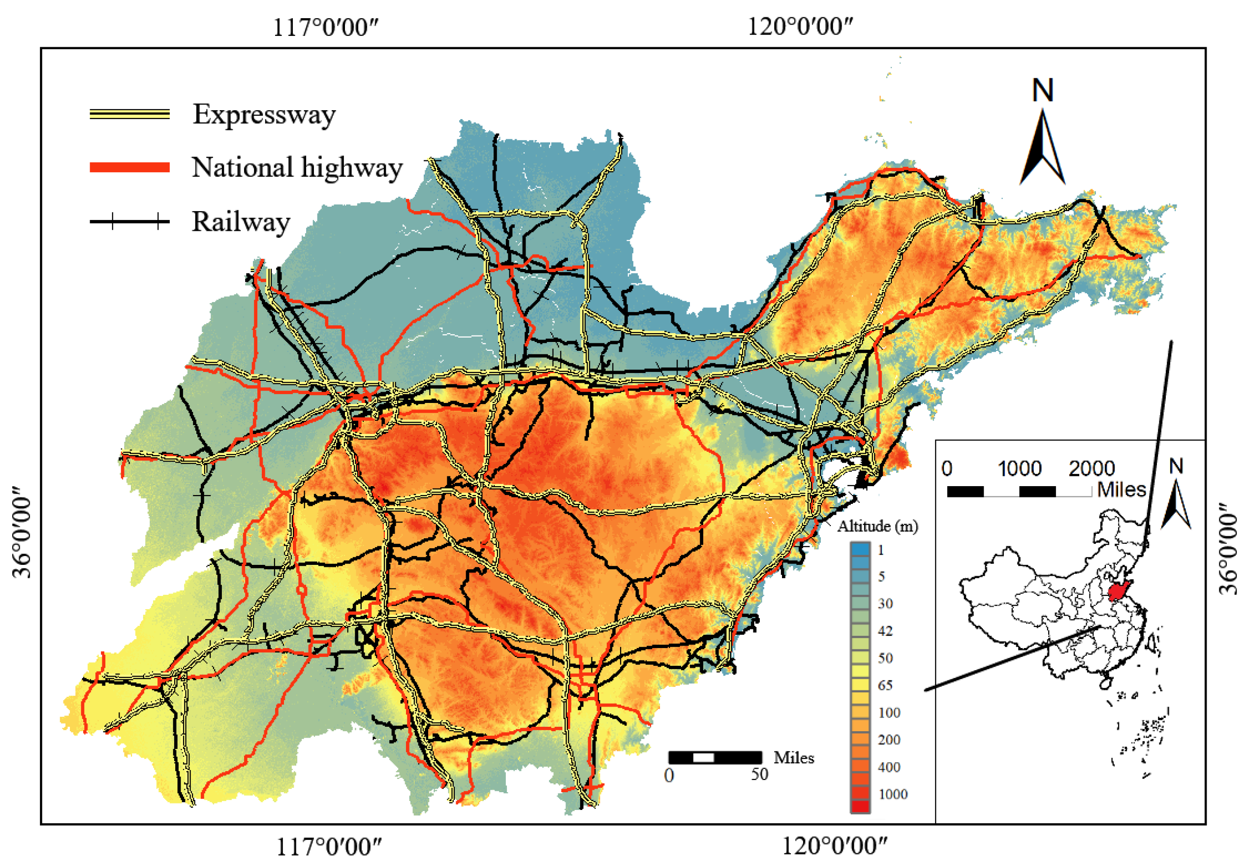
2.1. Study Domain

Shandong Province is located on the eastern coast of China, and it is located within 34°22.9′ N to 38°24.01′ N latitudes and 114°47.5′ E to 122°42.3′ E longitudes (Figure 1). In 2021, Shandong Province’s GDP reached 8.31 trillion yuan (RMB), with a population of approximately 101.7 million people. The robust industrial system has led to significant energy consumption, with the total energy consumption reaching 413.9 million tons of standard coal, which accounts for 8.5% of the country’s total energy consumption [27]. This high energy consumption is a major cause of serious pollution in some areas of Shandong. To address these environmental challenges, the government has implemented a series of measures, including strengthening the regulation of highly polluting and energy-consuming industries, promoting the adoption of cleaner production technologies, and fostering the development of green industries. These measures have reduced Shandong’s energy consumption per unit of GDP from 0.90 in 2010 to 0.53 in 2021. While there has been progress, it still lags behind the national average [28,29].

2.2. Source Categorization

Scientific and comprehensive classification of emission sources is an important basis for the establishment of reliable emission inventories [30]. The energy emissions of GHGs are typically divided into the following four categories: fossil fuel combustion, biomass combustion, coal mining and post-mine activities escape emissions, and oil and gas system escape emissions [31]. Air pollutants come from various sources, which can be categorized into eight primary types: stationary combustion, industrial process, road mobile sources, non-road mobile sources, solvent, dust, agricultural, and biomass combustion [32,33].

Given these classifications, this study proposes a unified classification method that applies the same categories of emission sources to both GHGs and air pollutants resulting from energy emissions. In this reclassification, stationary combustion includes power plants, heating plants, industries, and residents. Meanwhile, transportation modes such as highways, waterways, railways, and aviation, as well as agricultural machinery, are classified as either road mobile sources or non-road mobile sources, depending on their main area of operation. Open burning of biomass and rural residential burning are classified as biomass burning sources.

Emissions generated during non-energy consumption processes, such as coal mining and post-mining emissions, solvents, and emissions from agricultural activities, are not included in this classification. A detailed classification of emission sources is shown in Table S1.

2.3. Calculation Method and Data Collection

In this study, the emission factor method is combined with the material balance method to estimate emissions using activity data, emission factors, and control measures. The activity data for energy consumption across various sectors are sourced from the Energy Balance Sheet of Shandong Province (https://www.stats.gov.cn/sj/ndsj/, accessed on 17 December 2023). Vehicle information is obtained from the Shandong Statistical Yearbook (http://tjj.shandong.gov.cn/col/col6279/index.html, accessed on 17 December 2023). The latitude and longitude coordinates, as well as the installed capacity of units for 341 thermal power plants and heating plants, are derived from field research. The aircraft landing and take-off (LTO) cycle data are sourced from the Civil Transport Airport Production Statistics Bulletin published by the Ministry of Transport of the People’s Republic of China. Biomass burning data are obtained from the Shandong Provincial Rural Agricultural Bureau (http://nync.shandong.gov.cn/, accessed on 17 December 2023). In order to ensure the accuracy of the estimation, priority is given to the emission factors from Shandong Province and neighboring regions. The emission factors are shown in Tables S2–S5.

The emissions for GHGs, NOx, PM₁₀, PM_2.5, CO, volatile organic compounds (VOCs), and Ammonia (NH₃) were estimated using the emission factor method recommended by the IPCC [34], as shown in Equation (1):

$$\begin{array}{c}{E}_{ }=EF\times A\times \left(1-\eta \right)\end{array}$$

(1)

where, $E_{ }$ is the emissions of each pollutant from each source; $EF$ is the emission factor; $A$ is activity data; $\eta$ is removal efficiency. This study refers to the measurement and investigation of various pollutants and emission source subclasses in the literature. The specific methods are as follows:

The SO₂ emissions from power plants, heating plants, and motor vehicles were calculated using the material balance method. In this study, 341 thermal power plants and heating plants in Shandong Province were investigated. The investigation involved collecting information about their geographical location, fuel type, sulfur content, ash content, fly ash ratio, particle mass percentage, boiler type, process type, and removal facilities [35]. In recent years, with the continuous improvement of national gasoline standards, the quality of fuel used by railways and vehicles has also significantly improved [36]. The estimation equations are as follows.

$$\begin{array}{c}{E}_{S{O}_2}=\frac{64}{32}·A_{ }\times W_{ }\times S_{ }\times \left(1-\eta \right)\end{array}$$

(2)

$$\begin{array}{c}{E}_{SO2}=2.0\times {10}^{-6}\times \left(F_g\times a_g+F_d\times a_d\right)\end{array}$$

(3)

where $E_{S{O}_2}$ stands for SO₂ emissions; $\frac{64}{32}$ indicates the molecular weight ratio of SO₂ to S; $A$ is activity data; $W_{ }$ is the sulfur content of the fuel; $S_{ }$ is the release rate of sulfur; $\eta$ is removal efficiency. $F_g$ and $F_d$ are the consumption of gasoline and diesel of motor vehicles in this region, and the unit is t; $a_g$ and $a_d$ are the average sulfur content of motor vehicle gasoline and diesel oil in the region, with the unit of one part per million (ppm) by mass.

Emission estimation methods for aircraft [37], road mobile sources [38], and biomass combustion [39] are significantly influenced by factors such as landing times, mileage, and burn conditions of straw, which differ from the conventional emission factor method. The estimation method is as follows:

$$\begin{array}{c}{E}_i=\sum {MP}_i\times {VKT}_i\times EF\end{array}$$

(4)

$$\begin{array}{c}{E}_{i,m}=\sum n\times F_m\times E{F}_{i,m}\times t_{i,m}\end{array}$$

(5)

$$\begin{array}{c}{E}_{i,k}=P_k\times N_k\times R_k\times D_k\times {CE}_k\times E{F}_{i,k}\end{array}$$

(6)

where $i$ represents the types of pollutants and $E$ represents the total emissions; $MP$ represents the number of motor vehicles; $VKT$ represents the average annual mileage of all types of motor vehicles; $m$ is the phase of aircraft operation (approach, taxi, take-off, and climb); t indicates the time of phase $m$. $k$ stands for crop type; $p$ is the single yield of specific crops per year; $N$ is the ratio of grain to grass for each straw type; $R$ is the ratio of straw burning in a household or field; $D$ is the dry matter fraction of each straw type; $CE$ is the combustion efficiency of each straw type. Biomass will absorb CO₂ during the growth process, and the CO₂ emitted by combustion is basically the same as that absorbed, so it is no longer calculated.

2.4. Temporal and Spatial Allocation

Accurate spatial and temporal allocation is essential for constructing high-resolution emission inventories in order to understand localized emission characteristics. To consider emissions from different sources, appropriate spatial distribution weights were applied, and a high-resolution emission map of 5 km × 5 km was created using ArcGIS software (10.2). Emission data from point sources, such as power plants, heating plants, and airports, was allocated based on their installed capacity and takeoff and landing frequencies. Emissions from factories and commercial establishments were mapped based on GDP distribution, while residential consumption was mapped based on population distribution. The distribution of indoor biomass burning coincided with the residential areas on the land use type map, while outdoor biomass burning and agricultural machinery were allocated relative to the size of agricultural land. Railways and motor vehicles followed the distribution of their respective networks. The GDP grid data, population grid data, land use type distribution data, and road mobile sources data used in this study were obtained from the Data Center for Resources and Environmental Sciences, Chinese Academy of Sciences (http://www.resdc.cn, accessed on 22 March 2023). The power load curve of the power grid, the use of seasonal heating equipment, straw use and burning, and additional relevant data are utilized as the basis for allocating seasonal variations. Meanwhile, the congestion delay index serves as the basis for the daily variation allocation in on-road sources, as detailed in Tables S6 and S7.

2.5. Extended STIRPAT Model

The STIRPAT model overcomes the limitation of assuming a proportional relationship between IPAT factors and dependent variables. In addition to the basic P, A, and T factors, the STIRPAT model can incorporate other potential explanatory variables, thereby enhancing the flexibility and randomness of the model. The general form of the STIRPAT model is as follows:

$$\begin{array}{c}I=a{P}^{b^{\mathrm{\prime }}}{A}^{c^{\mathrm{\prime }}}{T}^{d^{\mathrm{\prime }}}e\end{array}$$

(7)

where, $I$, $P$, $A$, and $T$ represent environmental impact, population size, affluence, and technology, respectively. $a$ is the constant, $b$, $c$, and $d$ are the exponents of $P$, $A$, and $T$, respectively, and $e$ denotes the error term.

To address heteroscedasticity in the model, restrict the data range and apply a logarithmic transformation to the variables. This transformation helps convert the nonlinear relationship into a linear one, making it easier to interpret. The formula for the logarithmic transformation is as follows:

$$\begin{array}{c}lnI=lna+bln{P}_1+c_{1}ln{A}_1+c_{2}ln{A}_2+d_{1}ln{T}_1+d_{2}ln{T}_2+d_{3}ln{T}_3+lne\end{array}$$

(8)

where $I$ denotes the GHGs equivalent or atmospheric pollutant equivalent [40], $lna$ denotes the constant term, $P_1$ represents population size, $A_1$ stands for per capita real GDP, $A_2$ is the proportion of the secondary industry, $T_1$ signifies energy consumption, $T_2$ indicates energy consumption intensity, and $T_3$ refers to patent inventions. The elasticities for the model indicators are given by $b$, $c_1$, $c_2,d_1$, $d_2$, and $d_3$ respectively.

2.6. Scenario Setting

By combining the STIRPAT model and scenario analysis, with 2010–2021 as the base period, this study predicts the pathways to carbon peaking and the impact on pollutants under different scenarios from 2022 to 2035. The data for scenario predictions are sourced from the long-term development plan of Shandong Province and relevant literature [41,42], such as the “Long-term Trend Forecast of China’s Population” [43] and the “14th Five-Year Plan and 2035 Vision Outline for the National Economy and Social Development of Shandong Province” [44]. Five scenarios were established in this study: baseline scenario (BAU), high-speed development scenario (HSD), stable carbon peaking scenario (SCP), balanced emission reduction scenario (BER), and green emission reduction scenario (GER). The BAU is based on current policies and historical development trends. The HSD prioritizes economic growth compared to the other peaking scenarios. The SCP adjusts all indicators according to the government’s latest energy planning documents. The BER considers both economic and energy use factors, while the GER prioritizes environmental protection by adjusting adverse factors to the environment with a view to reaching an early peak (Table S12).

3. Results and Discussion

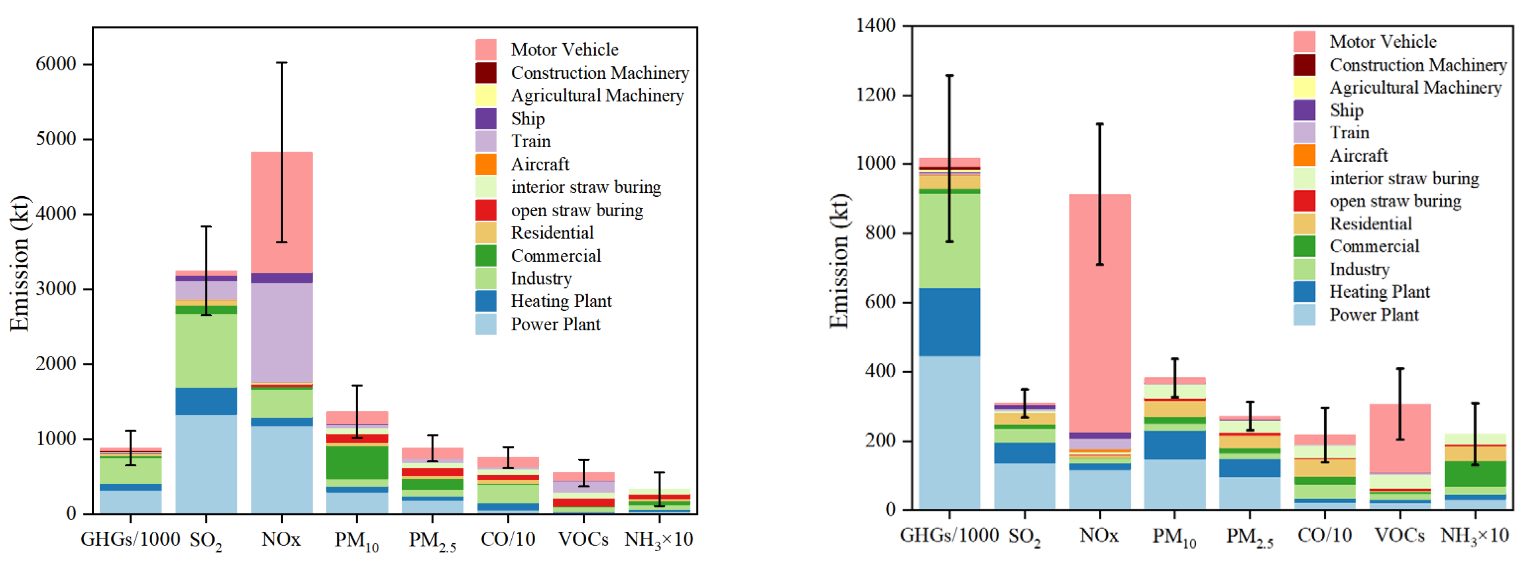
3.1. Emissions and Source Distribution of GHGs and Air Pollutants

GHGs from energy activities in Shandong Province have shown an overall rise, from 872.2 Mt CO₂eq to 1017.23 Mt CO₂eq in 2021 (as shown in Figure 2). This corresponds with the general upward trend in China’s CO₂ emissions observed by the IEA [45]. In this study, there are some variations in GHG emissions between 2013 and 2020. The small decrease in 2013 may be related to the implementation of the air control strategy in that year, especially the emission limitation policy for highly polluting enterprises. The decline in 2020 is closely related to the impact of COVID-19 on production and life. In contrast, air pollutant emissions show a downward trend from 2010 to 2021. Emissions of SO₂, NOx, PM₁₀, PM_2.5, CO, VOCs, and NH₃ from 3245.47, 4846.83, 1617.29, 973.88, 7860.38, 549.94, and 37.19 kt, respectively, to 308.83, 913.00, 425.81, 273.08, 1815.00, 299.79, and 13.04 kt. Among them, the concentration of SO₂ and NOx decreased most significantly, by 90% and 81%, respectively, especially in the period from 2013 to 2017, when the average annual decline reached 25% and 20%, respectively (as shown in Figure 2). The emission reduction effect of VOCs and CO has been gradually significant since 2018, which means that at different time nodes and for different pollutants, the emission reduction strategy has been timely adjusted and optimized.

Stationary combustion is the main source of GHGs and atmospheric pollutants, contributing 95% of GHGs, 90% of SO₂, and over 70% of PM₁₀, PM_2.5, CO, and NH₃ (as shown in Figure 3). Power plants have been using cleaner coal and increasing end-of-pipe measures to reduce emissions. The emissions of SO₂, NOx, PM₁₀, and PM_2.5 have been reduced from 1335.30, 1176.19, 291.86, and 188.30 kt to 135.98, 116.70, 148.15, and 95.58 kt, achieving a reduction of approximately 89.81%, 90.07%, 49.25%, and 49.23% (as shown in Figure 3). Although power plants have implemented ultra-low emission measures, as they are the main sector of coal consumption, they still contribute more than 30% of SO₂, PM₁₀, and PM_2.5 emissions. Additionally, the industrial sector, with its large-scale energy consumption, contributes to over one-third of GHG emissions and 13% and 19% of SO₂ and CO emissions, respectively.

Since 2013, Shandong has been implementing the “coal-to-gas” strategy, progressively adjusting its energy consumption structure. Consequently, coal consumption in the commercial sector has significantly decreased from 8357.3 thousand tons in 2010 to 2135.2 thousand tons in 2021. However, residential coal consumption has shown a fluctuating trend, primarily due to the variability in natural gas prices and the initial capital investment required for policy implementation. As a result, some residents continue to prefer using coal, a cheaper and more reliable source of energy for heating and cooking. Between 2010 and 2021, emissions from commercial and residential sources were reduced by 90% and 50%, respectively (Figure 3). In response, the government implemented subsidy policies in 2017 to improve the central heating infrastructure and provide residents with more economical and environmentally friendly energy options. These efforts have gradually transformed energy consumption. According to the green energy development action plan of the “Hundred Townships and Thousand Villages” in Shandong Province, there is still a significant disparity in the energy consumption structure between urban and rural areas. Specifically, rural residents have a per capita coal consumption of 192 kg, which is 4.2 times higher than that of urban residents. This indicates the potential to reduce emissions.

Road sources are the main sources of NOx and VOC emissions from fossil energy consumption, accounting for 75% and 64% of total emissions, respectively. Due to the operating mechanism of diesel engines, heavy trucks have become the main source of NOx emissions, accounting for 70–85% of motor vehicle emissions. Because of their large numbers, light passenger cars are identified as the largest emitters of CO and VOCs, accounting for 51% and 62% of all vehicle emissions in 2021 (Figure 4). Despite the continuous increase in the number of motor vehicles, the total emissions of air pollutants caused by these vehicles have shown an overall downward trend, thanks to the continuous improvement of national emission standards. However, we also observed a slight rebound in pollutant emissions as the number of vehicles increased between the two updates to emission standards.

Railway turnover in Shandong Province showed a decreasing trend from 2011 to 2015. However, driven by the “road-to-rail transfer” policy, freight turnover increased from 107,728 million ton-kilometers to 168,212 million ton-kilometers between 2015 and 2021. Especially after 2018, Shandong actively implemented the Three-year Action Plan for Promoting Transportation Structural Adjustment (2018–2020), which resulted in an annual growth rate of 8.25% in freight turnover. Nonetheless, the expansion of railway electrification, along with the improvement of internal combustion locomotives and the implementation of stricter fuel standards, has resulted in a significant reduction in pollutant emissions. For example, SO₂ emissions were reduced from 238.9 kt to 5.6 kt, a 97% reduction. However, there is still potential for rail transport to reduce emissions as the electrification of railroads advances and transport efficiency continues to be optimized.

In 2010, biomass combustion was the main contributor to emissions of particulate matter, CO, VOCs, and NH₃, with VOCs and NH3 accounting for a third of these emissions (Figure 5). Outdoor biomass combustion was found to produce more pollutants compared to indoor combustion due to incomplete combustion, posing a considerable environmental threat at that time [46]. However, with the implementation of measures to ban straw burning, the proportion of straw burning has decreased year by year. By 2020, widespread straw burning had become rare. Simultaneously, the increased adoption of clean energy significantly reduced the reliance on direct biomass usage as fuel. According to the Notice on Further Strengthening the Improvement of Rural Living Environment jointly issued by the Shandong Provincial Development and Reform Commission and the Rural Department, the proportion of straw burning has significantly decreased. Fuelwood usage as the primary energy source in rural areas decreased to 14.8 percent in 2019, compared to 28.1 percent in 2010.

3.2. Temporal and Spatial Distribution Characteristics

3.2.1. Spatial Distribution

On the distribution map of a 5 km × 5 km area, there are significant regional differences in the levels of SO₂, NOx, PM₁₀, PM_2.5, CO, VOCs, NH₃, and GHGs in Shandong Province in 2010 and 2021. As shown in Figure 6, the eastern coastal and central areas are regions with relatively concentrated emissions. There is significant heterogeneity in the spatial distribution of various pollutants. For example, in the western and southwestern parts of Shandong province, where there is more agricultural land, the concentrations of pollutants such as PM₁₀, PM_2.5, CO, VOCs, and NH₃ are higher. Additionally, pollutants such as NOx, CO, and VOCs, which are closely associated with vehicular activities, exhibit a clear linear distribution pattern. There are significant differences in the emission intensity of GHGs and pollutants. The concentration of GHG far exceeds that of other atmospheric pollutants by a factor of several thousand. The emission of CO is almost equivalent to the combined emissions of other atmospheric pollutants.

Simultaneously, comparing the spatial distribution of pollutants in 2021 and 2010, the maximum value of GHG emissions in 2021 increases significantly. The area of high-value regions has expanded. This suggests that GHG emissions increase significantly in some areas over the 12-year period and that a wider area begins to face higher GHG emissions. Conversely, the situation with atmospheric pollutants shows an optimistic transformation. In 2021, there is a decrease in high-value regions, and they appear to be more widely distributed. This may imply that the sources of high pollution have become more dispersed or that control measures in certain areas have been effective (Figure 6). Overall, these two sets of comparative images depict a complex phenomenon. Over the past 12 years, significant progress has been made in combating air pollutants. However, there is still considerable pressure to reduce GHG emissions. This discrepancy highlights the imbalance in environmental protection efforts, and so there is a need to strengthen GHG reduction measures.

To further delve into the characterization of emission spatial heterogeneity, the probability distributions of GHGs and air pollutants are shown in Figure S1. In general, most of the emissions are concentrated in a small area. The top 10% of grids for SO₂, NOx, PM₁₀, PM_2.5, CO, VOCs, NH₃, and GHG emissions account for 58%, 59%, 56%, 58%, 37%, 53%, 46%, and 72% of the total emissions. And SO₂, PM₁₀, PM_2.5, CO, and VOCs account for more than 50% of grids that emit 72% of GHGs and indicate strong spatial consistencies between the air pollutants and GHG emissions.

3.2.2. Temporal Variation

As shown in Figure 7, emissions of GHGs and air pollutants in 2010 and 2021 are higher in summer and winter than in other seasons. This is mainly due to the increased consumption of fossil fuels in power plants, driven by the widespread use of refrigeration equipment in summer and the increased demand for heating in Shandong Province during winter, coupled with the intensification of production activities in factories leading up to the Chinese New Year. Additionally, in 2010, emissions of PM_2.5, PM₁₀, VOCs, and NH₃ were significantly higher from May to August compared to other periods, predominantly due to more widespread straw burning. However, in 2021, emissions of these pollutants did not show significant peaks in other months, likely due to a decrease in straw burning practices.

On the daily time scale, the emission pattern of pollutants is highly consistent with people’s daily travel and activity habits (Figure S1). The peak of pollutant emissions is mainly concentrated between 6:00 and 22:00. Specifically, pollutant emissions reach their daily maximum between 6:00 and 9:00 and between 17:00 and 19:00. This coincides with peak hours when people are commuting. This synchronicity suggests that daily socio-economic activities have a significant impact on short-term fluctuations in air quality.

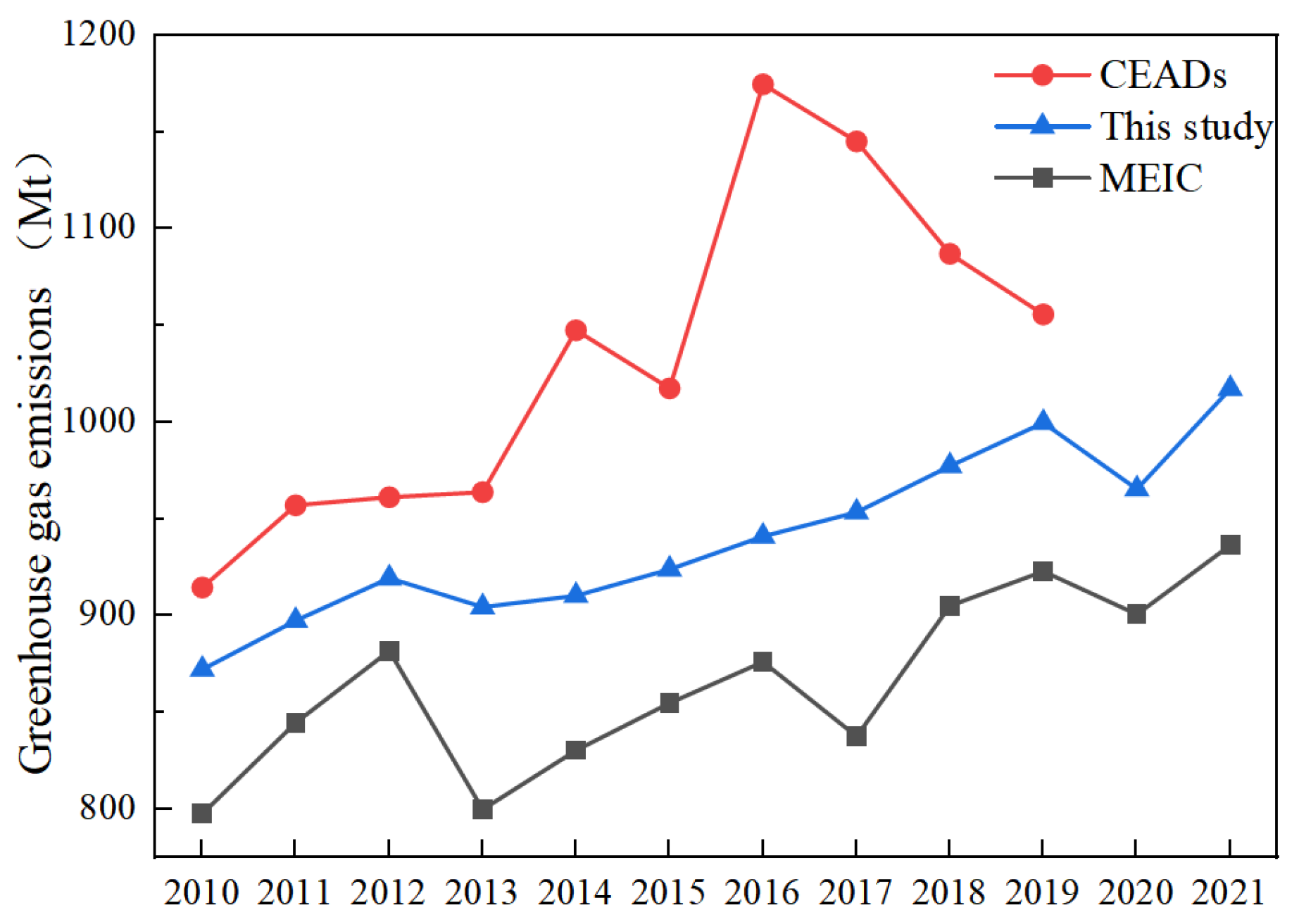
3.3. Comparison and Evaluation of Emission Inventory

In order to verify the accuracy and reliability of the inventory compilation, this study utilized two authoritative databases, namely the Carbon Emission Accounts and Datasets (CEADs) (https://www.ceads.net.cn/, accessed on 22 March 2023) and Multi-resolution Emission Inventory for China (MEIC) (http://meicmodel.org.cn/, accessed on 22 March 2023), to conduct a comprehensive comparison of GHG emission data over time. Due to the limited availability of long-term air pollutant research data, this paper chose to utilize cross-sectional data and compare it with local research findings in Shandong Province.

The GHG emission trends obtained in this study are generally consistent with the results of the MEIC database [47], but the calculated emissions are slightly higher (Figure 8). This difference is mainly due to the additional consideration of CH₄ and N₂O emissions in our calculations. Compared to this study and MEIC, the GHG emissions recorded in the carbon accounting database are more significant. This is primarily because the database not only includes GHG generated by the combustion of fossil fuels but also encompasses emissions from industrial production processes [48]. For example, the calcination of calcium carbonate in cement production results in a large amount of CO₂.

When assessing atmospheric pollutant emissions, SO₂ emissions were estimated to be 400.74 kt in this study (

Table 1. Comparison with air pollutant emission inventories for Shandong Province (Unit: kt).

Reference	Year	Sources	SO2	NOx	PM10	PM2.5	CO	VOCs	NH3
Zheng et al. [49]	2017	Power plants	159.21	410.09	105.89	61.37	457.93	8.17	0.00
		Industries	615.64	897.22	495.76	342.18	4529.54	1929.22	32.60
		Residents	152.85	72.06	227.44	204.41	3862.14	412.66	19.41
		Road mobile	32.59	763.59	70.63	68.57	2518.58	445.06	4.07
		Agriculture	0.00	0.00	0.00	0.00	0.00	0.00	661.85
		Total	960.29	2142.96	899.72	676.53	11368.19	2795.10	717.93
Jiang et al. [50]	2016	Fossil fuel combustion	157.40	254.70	900.40	493.30	2902.20	71.50	0.00
		Biomass burning	57.50	75.10	359.50	341.40	4416.70	359.20	0.00
		Road mobile	0.00	985.80	49.20	35.70	1537.00	269.90	0.00
		Total	214.90	1315.60	1309.10	870.40	8855.90	700.60	0.00
This study	2017	Power plants	192.16	252.42	153.67	99.14	327.15	20.67	2.81
		Industries	145.81	82.58	54.60	47.78	1501.43	40.77	5.34
		Residents	50.08	7.04	49.66	38.34	547.71	3.13	3.13
		Biomass burning	8.51	17.72	74.93	69.62	606.98	73.39	5.01
		Road mobile	4.19	618.01	63.90	63.90	1778.84	225.20	0.00
		Total	400.74	977.77	396.77	318.78	4762.11	363.17	16.29

). This is significantly lower than the 960.29 kt reported by Zheng et al. [49], primarily because we did not include emissions from industrial processes. However, when considering only emissions from power and thermal plants, our estimates closely align with Zheng et al. [49]. The value being higher than that of Jiang et al. [50] at 214.90 kt might be attributed to increased coal consumption in our study year and the implementation of more aggressive sulfur removal measures by Jiang et al. [50].

Motor vehicles are the primary source of NOx emissions. According to Zheng et al. [49] and our data, the NOx emissions reached 763.59 kt and 618.01 kt, respectively. Both values are significantly lower than the 988.5 kt reported by Jiang et al. [50]. Jiang et al. [50] utilized a more sophisticated Copert V5 model for their estimation, which enhanced the scientific accuracy of their data. In contrast, our estimation with Zheng et al. [49] is primarily based on simplified fuel consumption, which may not fully consider important factors such as environmental background and driving characteristics.

In the study of particulate matter emissions, we observe that Zhang et al. [49] pay more attention to the contribution of industrial processes, whereas our study with Jiang et al. [50] focuses on the impact of fossil fuel combustion. Nonetheless, consistent with Zheng et al., we also consider residential activity as a key source of particulate matter emissions. These activities also emit significant amounts of CO, which primarily comes from industrial and biomass combustion. Interestingly, our emission estimates regarding biomass burning are much lower than those of Jiang et al. [50]. This may be related to the straw-burning exclusion operation conducted in Shandong Province in 2016, which effectively reduced incidents of open burning.

In terms of VOC emissions, the primary sources identified in this paper differ from those in the other two research studies. Zheng et al. [49] identify industrial sources as the major contributors. Their categorization of industrial sources includes both the combustion of industrial fossil fuels and industrial process emissions, with the latter being identified as the primary source of VOCs [30]. In contrast, Jiang et al. [50]. show a higher proportion of VOCs originating from biomass combustion. Additionally, all three studies concur that motor vehicles are a significant source of VOC emissions.

Overall, our findings are generally in agreement with previous studies that have demonstrated similar emission trends. This provides reliability validation for our research methodology and a solid foundation for future studies.

3.4. Uncertainty Analysis

The uncertainty of the emission inventory arises from a combination of uncertainties in emission factors, removal efficiencies, and activity data. In this study, the Monte Carlo simulation method was used to quantitatively evaluate the uncertainty of the estimated results, with further details available in Cai et al. [51]. This simulation was executed 10,000 times with a 95% confidence interval to derive the uncertainty ranges. The estimated range of emissions of GHGs and atmospheric pollutants is shown in Figure 5, and specific data are shown in Table S8.

The uncertainty in SO₂ emissions is the smallest, primarily because the material balance method is used heavily in the evaluation process. For instance, the sulfur content in fossil fuels and the removal efficiency of devices are determined based on local data from Shandong Province. Additionally, the activity data, sourced entirely from the official statistics of Shandong Province, are highly credible. However, for pollutants such as CO, VOCs, and NH₃, the uncertainty is relatively higher due to the limited availability of local data, necessitating the sourcing of some information from literature in other regions. In terms of emission sources, non-road sources and biomass combustion exhibit significant uncertainty, primarily due to the lack of extensive field surveys and the incompleteness of data regarding open straw burning sourced from the Rural Agriculture Department.

3.5. Analysis of Driving Factors

The ordinary least squares (OLS) method was used to analyze the correlation between GHGs, air pollutant equivalents, population, per capita GDP, proportion of secondary industry, energy consumption, energy intensity, and patented inventions. It was found that the variance inflation factor (VIF) of each factor was greater than 10, indicating that there was a serious collinearity problem among the model variables (Table S9). In order to prevent the distortion of the model fitted by the OLS method, the ridge regression method is used to eliminate multicollinearity between variables (Tables S10 and S11). The prediction models of GHGs and air pollutants constructed are as follows:

$$\begin{array}{c}ln{I}_1=0.346ln{P}_1+0.035ln{A}_1-0.062ln{A}_2+0.050ln{T}_1-0.053ln{T}_2+0.008ln{T}_3+9.804\end{array}$$

(9)

$$\begin{array}{l}ln{I}_2=-4.833n{P}_1-0.49136ln{A}_1+0.909ln{A}_2+1.060ln{T}_1+0.570ln{T}_2-0.127n{T}_3\\ \hspace{1em}\hspace{1em}\hspace{1em}\hspace{1em}\hspace{1em} +49.591\end{array}$$

(10)

According to the prediction model, various factors have different degrees of influence and directions on the levels of GHGs and air pollutants. However, the variables with the greatest influence are population, the proportion of secondary industry, energy consumption, and energy consumption intensity. In many studies on the influence factors of GHGs or air pollutants, the most influential factor is population, which is consistent with the research conclusion of this paper [41,52,53]. A large population leads to more production and energy consumption, but population growth pushes people to concentrate in resource-rich areas, which can promote more intensive and efficient energy use. The factors that have the least impact of patent innovation on GHGs and air pollutants may be because there is a time lag in the wide application of new technologies, which cannot be rapidly promoted, and some end-treatment technologies for air pollutants may lead to an increase in GHGs. For example, limestone reacts with SO₂ to release CO₂, and increased electricity demand may also indirectly increase CO₂ emissions.

There is a strong agreement between the estimated value and the STIRPAT output of GHG and air pollutant equivalent emissions from energy consumption in Shandong Province. Specifically, the error rate of GHGs as a whole is maintained in the range of ±3%, while the error rate of atmospheric pollutant equivalent is located in the range of −15% to −20%, and the prediction model can be used for predictive analysis (Figure S3).

3.6. Scenario Prediction

In the five scenarios studied, the BAU and HSD failed to reach the peak of GHG emissions before 2030, while the SCP, BER, and GER successfully achieved this goal, particularly the GER, which even reached it by 2027 (Figure 9). In the BAU, Shandong’s GHG emissions are consistently increasing, with an average annual growth rate of 0.34% from 2022 to 2035. This growth rate is lower than the 1.86% observed from 2010 to 2021, but it still does not meet the country’s carbon peak target by 2030. Therefore, this scenario is clearly not desirable. For the HSD, though again not peaking before 2030, growth has slowed to an average annual rate of 0.24%.

Both the SCP and the BER achieve the peak of GHG in 2030, but their paths and peaks are different. The SCP is based on a set of medium parameters such as fertility and economic growth, while the BER focuses on the quality of life by combining high economic growth, low energy consumption, and a high volume of patented inventions. In contrast, the BER would result in 31.5 Mt CO₂eq less cumulative GHG emissions in 2022–2035 compared to the peaking scenario. The GER peaks at 1009.3 Mt CO₂eq of GHG emissions in 2027. However, this requires lower energy consumption, lower fertility, and lower per capita GDP growth. This suggests that sacrificing certain economic and demographic factors for environmental quality may not be a viable option in the long run.

The air pollutant equivalent showed a downward trend in different development scenarios, indicating active efforts to reduce air pollutant emissions in each scenario. However, the rate of decline varies in different scenarios. In the BAU, the rate of reduction by 2028 is lower than in the other four scenarios. Unexpectedly, after 2028, the air pollutant equivalents of the HSD and the GER will be higher than those of the BAU. This finding leads us to rethink that pursuing economic growth alone, or focusing too much on peaking carbon emissions, may not be consistent with long-term sustainability. In addition, the SCP and BER have achieved significant results in reducing air pollutants, demonstrating that striking a balance between economic growth and environmental protection is both practical and feasible. More importantly, such balancing strategies are likely to have long-term and lasting positive effects. This study highlights the need to adopt a global perspective and long-term planning in the formulation of relevant policies, integrating multiple elements to help us achieve the best balance between economic growth and environmental protection. This research result not only has reference value for future policy setting but also highlights the importance of balanced economic and environmental development and points out the direction for subsequent related research.

4. Conclusions and Policy Implications

Based on a regionally adapted research method and the STIRPAT model, this paper systematically discusses the emission characteristics, spatial distribution, influencing factors, and future trends of GHGs and air pollutants resulting from energy consumption in Shandong Province. Firstly, this study estimates the unified emission inventory of GHGs and air pollutants at the same subsector level. It combines the emission factor method and the material balance method to estimate the emissions associated with historical energy consumption. Based on the appropriate spatial weight factors, the ArcGIS software was used to analyze the spatial distribution characteristics of various GHGs and air pollutants. The STIRPAT model is used to analyze the contribution of each driving factor to emissions, forecast the future carbon peak through scenario analysis, and estimate the emissions of pollutants along each peak path. Therefore, a comprehensive evaluation and prediction model have been established.

The results showed that: (1) From 2010 to 2021, Shandong Province successfully reduced the emission of air pollutants from energy consumption, while the emission of GHGs increased. Stationary combustion and on-road emissions are the most important sources of emissions, indicating that improving energy structures is conducive to reducing pollution and carbon emissions. (2) The overall distribution of GHGs and air pollutants is similar, with emissions mainly concentrated in the eastern coastal and central areas of Shandong Province. This concentration makes collaborative control efforts more feasible. (3) The STIRPAT model was utilized to analyze the underlying factors of GHG and air pollutant emissions in energy consumption within Shandong Province. This study revealed that population was identified as the most significant factor influencing the emissions of GHGs and air pollutants. This finding aligns with the conclusions drawn from previous research studies. (4) By comparing emissions and their trends under different scenarios, we observe that the predicted carbon peak will be achieved before 2030 in SCP, BER, and GER. Specifically, GER predicts that this goal will be achieved in 2027. However, blindly pursuing economic growth or solely focusing on carbon peaking is not a sustainable option in the long run. SCP and BER confirm that achieving a balance between the economy and the environment is possible and can have a lasting positive impact on the future.

The research results of this paper can provide policy references for Shandong Province to reduce pollution and carbon emissions. (1) In view of the current development trend, in order to achieve the carbon peak target, Shandong Province should adopt more stringent carbon emission reduction measures. (2) To optimize energy allocation, it is imperative to bolster green innovation capabilities and further diminish dependence on coal consumption. (3) To facilitate the shift to a green economy, a progressive reduction in reliance on high-energy-consuming traditional industries and an adjustment of the industrial layout are essential. (4) To advance the notion of sustainable living, it is recommended to bolster public participation and establish a consumption framework aligned with the principles of circular and sharing economies.

Finally, although this study estimated a high-resolution unified emission inventory of GHGs and air pollutants at the same subsector level of energy consumption in Shandong Province from 2010 to 2021 using localized data, the STIRPAT model and scenario analysis were employed to investigate their drivers and future development trends. However, there are still some limitations. Firstly, during the process of compiling the inventory, the localized emission factors are not comprehensive enough and have significant uncertainties. Moreover, although the activity data are sourced from official records, they may exhibit a degree of latency, thereby affecting the timeliness and relevance of the information. Secondly, the compilation system of the homologous classification list of GHGs and air pollutants needs to be further improved and subdivided. Additionally, this study examines the impact and prediction of six drivers, but there may be additional factors that influence the research results. The interaction between GHGs and atmospheric pollutants is undoubtedly complex, and it has profound effects on human health and the environment. In order to achieve the dual goals of reducing pollution and carbon emissions, the collaborative control strategy between the two is particularly crucial and warrants further exploration.

References

1. Yuan, R.; Ma, Q.; Zhang, Q.; Yuan, X.; Wang, Q.; Luo, C. Coordinated Effects of Energy Transition on Air Pollution Mitigation and CO2 Emission Control in China. Sci. Total Environ. 2022, 841, 156482. [Google Scholar] [CrossRef]
2. Xu, C.; Zhang, Z.; Ling, G.; Wang, G.; Wang, M. Air Pollutant Spatiotemporal Evolution Characteristics and Effects on Human Health in North China. Chemosphere 2022, 294, 133814. [Google Scholar] [CrossRef]
3. Lao, J.; Song, H.; Wang, C.; Zhou, Y.; Wang, J. Reducing Atmospheric Pollutant and Greenhouse Gas Emissions of Heavy Duty Trucks by Substituting Diesel with Hydrogen in Beijing-Tianjin-Hebei-Shandong Region, China. Int. J. Hydrogen Energy 2021, 46, 18137–18152. [Google Scholar] [CrossRef]
4. WMO. Provisional State of the Global Climate in 2022. Available online: https://public.wmo.int/en/our-mandate/climate/wmo-statement-state-of-global-climate (accessed on 22 March 2023).
5. Deng, X.; Zou, B.; Li, S.; Wu, J.; Yao, C.; Shen, M.; Chen, J.; Li, S. Disease Specific Air Quality Health Index (AQHI) for Spatiotemporal Health Risk Assessment of Multi-Air Pollutants. Environ. Res. 2023, 231, 115943. [Google Scholar] [CrossRef]
6. IEA. Global Energy Review CO2 Emissions in 2021. 2021. Available online: https://iea.blob.core.windows.net/assets/d0031107-401d-4a2f-a48b-9eed19457335/GlobalEnergyReview2021.pdf (accessed on 17 December 2023).
7. MCEPRC. Ecological Environmental Bulletin of China. Available online: https://www.mee.gov.cn/hjzl/sthjzk/zghjzkgb/ (accessed on 22 March 2023).
8. Chen, W.; Tang, H.; He, L.; Zhang, Y.; Ma, W. Co-Effect Assessment on Regional Air Quality: A perspective of Policies and Measures with Greenhouse Gas Reduction Potential. Sci. Total Environ. 2022, 851, 158119. [Google Scholar] [CrossRef]
9. Nguyen, T.H.; Hung, N.T.; Nagashima, T.; Lam, Y.F.; Doan, Q.-V.; Kurokawa, J.; Chatani, S.; Derdouri, A.; Cheewaphongphan, P.; Khan, A.; et al. Development of Current and Future High-Resolution Gridded Emission Inventory of Anthropogenic Air Pollutants for Urban air Quality Studies in Hanoi, Vietnam. Urban Clim. 2022, 46, 101334. [Google Scholar] [CrossRef]
10. Marchi, M.; Capezzuoli, F.; Fantozzi, P.L.; Maccanti, M.; Pulselli, R.M.; Pulselli, F.M.; Marchettini, N. GHG Action Zone Identification at the Local Level: Emissions Inventory and Spatial Distribution as Methodologies for Policies and Plans. J. Clean. Prod. 2023, 386, 135783. [Google Scholar] [CrossRef]
11. Chatani, S.; Kitayama, K.; Itahashi, S.; Irie, H.; Shimadera, H. Effectiveness of Emission Controls Implemented since 2000 on Ambient Ozone Concentrations in Multiple Timescales in Japan: An emission Inventory Development and Simulation Study. Sci. Total Environ. 2023, 894, 165058. [Google Scholar] [CrossRef]
12. Paunu, V.-V.; Karvosenoja, N.; Segersson, D.; López-Aparicio, S.; Nielsen, O.-K.; Plejdrup, M.S.; Thorsteinsson, T.; Niemi, J.V.; Vo, D.T.; Denier van der Gon, H.A.C.; et al. Spatial Distribution of Residential Wood Combustion Emissions in the Nordic Countries: How Well National Inventories Represent Local Emissions? Atmos. Environ. 2021, 264, 118712. [Google Scholar] [CrossRef]
13. Qu, Y.; Cang, Y. Cost-Benefit Allocation of Collaborative Carbon Emissions Reduction Considering Fairness Concerns—A Case Study of the Yangtze River Delta, China. J. Environ. Manag. 2022, 321, 115853. [Google Scholar] [CrossRef]
14. Wang, L.; Wu, Z.; Wang, X. Multimodal Transportation and City carbon Emissions over Space and Time: Evidence from Guangdong-Hong Kong-Macao Greater Bay Area, China. J. Clean. Prod. 2023, 425, 138987. [Google Scholar] [CrossRef]
15. Wu, B.; Bai, X.; Liu, W.; Zhu, C.; Hao, Y.; Lin, S.; Liu, S.; Luo, L.; Liu, X.; Zhao, S.; et al. Variation Characteristics of Final Size-Segregated PM Emissions from Ultralow Emission Coal-Fired Power Plants in China. Environ. Pollut. 2020, 259, 113886. [Google Scholar] [CrossRef]
16. Zhao, Y.; Zhou, Y.; Qiu, L.; Zhang, J. Quantifying the Uncertainties of China’s Emission Inventory for Industrial Sources: From National to Provincial and City Scales. Atmos. Environ. 2017, 165, 207–221. [Google Scholar] [CrossRef]
17. Wu, T.; Cui, Y.; Lian, A.; Tian, Y.; Li, R.; Liu, X.; Yan, J.; Xue, Y.; Liu, H.; Wu, B. Vehicle Emissions of Primary Air Pollutants from 2009 to 2019 and Projection for the 14th Five-Year Plan Period in Beijing, China. J. Environ. Sci. 2023, 124, 513–521. [Google Scholar] [CrossRef]
18. Shi, Y.; Han, B.; Han, L.; Wei, Z. Uncovering the National and Regional Household Carbon Emissions in China Using Temporal and Spatial Decomposition Analysis Models. J. Clean. Prod. 2019, 232, 966–979. [Google Scholar] [CrossRef]
19. Gao, Y.; Zhang, L.; Huang, A.; Kou, W.; Bo, X.; Cai, B.; Qu, J. Unveiling the Spatial and Sectoral Characteristics of a High-Resolution Emission Inventory of CO2 and Air Pollutants in China. Sci. Total Environ. 2022, 847, 157623. [Google Scholar] [CrossRef]
20. Liu, X.; Peng, R.; Bai, C.; Chi, Y.; Liu, Y. Economic Cost, Energy Transition, and Pollutant Mitigation: The Effect of China’s Different Mitigation Pathways toward Carbon Neutrality. Energy 2023, 275, 127529. [Google Scholar] [CrossRef]
21. Luo, X.; Liu, C.; Zhao, H. Driving Factors and Emission Reduction Scenarios Analysis of CO2 Emissions in Guangdong-Hong Kong-Macao Greater Bay Area and Surrounding Cities Based on LMDI and System Dynamics. Sci. Total Environ. 2023, 870, 161966. [Google Scholar] [CrossRef]
22. Song, C.; Zhao, T.; Wang, J. Spatial-Temporal Analysis of China’s Regional Carbon Intensity Based on St-Ida from 2000 to 2015. J. Clean. Prod. 2019, 238, 117874. [Google Scholar] [CrossRef]
23. Ribeiro, L.C.D.S.; Filho, J.F.D.S.; Santos, G.F.D.; Freitas, L.F.D.S. Structural Decomposition Analysis of Brazilian Greenhouse Gas Emissions. World Dev. Sustain. 2023, 2, 100067. [Google Scholar] [CrossRef]
24. Wang, W.; Hu, Y.; Lu, Y. Driving Forces of China’s Provincial Bilateral Carbon Emissions and the Redefinition of Corresponding Responsibilities. Sci. Total Environ. 2023, 857, 159404. [Google Scholar] [CrossRef]
25. Yu, S.; Zhang, Q.; Hao, J.L.; Ma, W.; Sun, Y.; Wang, X.; Song, Y. Development of an Extended Stirpat Model to Assess the Driving Factors of Household Carbon Dioxide Emissions in China. J. Environ. Manag. 2023, 325, 116502. [Google Scholar] [CrossRef]
26. Xue, L.; Li, H.; Xu, C.; Zhao, X.; Zheng, Z.; Li, Y.; Liu, W. Impacts of Industrial Structure Adjustment, Upgrade and Coordination on Energy Efficiency: Empirical Research Based on the Extended STIRPAT Model. Energy Strategy Rev. 2022, 43, 100911. [Google Scholar] [CrossRef]
27. National Bureau of Statistics. China Statistical Yearbook. Available online: https://data.stats.gov.cn/ (accessed on 22 March 2023).
28. Liu, J.; Ma, H.; Wang, Q.; Tian, S.; Xu, Y.; Zhang, Y.; Yuan, X.; Ma, Q.; Xu, Y.; Yang, S. Optimization of Energy Consumption Structure Based on Carbon Emission Reduction Target: A Case Study in Shandong Province, China. Chin. J. Popul. Resour. Environ. 2022, 20, 125–135. [Google Scholar] [CrossRef]
29. Shandong Bureau of Statistics. Shandong Statistical Yearbook. Available online: http://tjj.shandong.gov.cn/tjnj/nj2021/zk/indexce.htm (accessed on 22 March 2023).
30. Zhang, B.; Yin, S.; Lu, X.; Wang, S.; Xu, Y. Development of City-Scale Air Pollutants and Greenhouse Gases Emission Inventory and Mitigation Strategies Assessment: A Case in Zhengzhou, Central China. Urban Clim. 2023, 48, 101419. [Google Scholar] [CrossRef]
31. Li, Y.; Du, W.; Huisingh, D. Challenges in Developing an Inventory of Greenhouse Gas Emissions of Chinese Cities: A Case Study of Beijing. J. Clean. Prod. 2017, 161, 1051–1063. [Google Scholar] [CrossRef]
32. Zhong, Z.; Zheng, J.; Zhu, M.; Huang, Z.; Zhang, Z.; Jia, G.; Wang, X.; Bian, Y.; Wang, Y.; Li, N. Recent Developments of Anthropogenic Air Pollutant Emission Inventories in Guangdong Province, China. Sci. Total Environ. 2018, 627, 1080–1092. [Google Scholar] [CrossRef]
33. Zhou, M.; Jiang, W.; Gao, W.; Gao, X.; Ma, M.; Ma, X. Anthropogenic Emission Inventory of Multiple Air Pollutants and Their Spatiotemporal Variations in 2017 for the Shandong Province, China. Environ. Pollut. 2021, 288, 117666. [Google Scholar] [CrossRef]
34. IPCC. 2006 IPCC Guidelines for National Greenhouse Gas Inventories. Available online: https://www.ipcc-nggip.iges.or.jp/public/2006gl/index.html (accessed on 7 July 2023).
35. Xiong, T.; Jiang, W.; Gao, W. Current Status and Prediction of Major Atmospheric Emissions from Coal-Fired Power Plants in Shandong Province, China. Atmos. Environ. 2016, 124, 46–52. [Google Scholar] [CrossRef]
36. Zhang, S. Technical Guide for Compiling Emission Inventories of Air Pollutants from Road Vehicles (Trial); Ministry of Environmental Protection: Beijing, China, 2015. [Google Scholar]
37. Han, B.; Wang, L.; Deng, Z.; Shi, Y.; Yu, J. Source Emission and Attribution of a Large Airport in Central China. Sci. Total Environ. 2022, 829, 154519. [Google Scholar] [CrossRef]
38. Zheng, B.; Huo, H.; Zhang, Q.; Yao, Z.L.; Wang, X.T.; Yang, X.F.; Liu, H.; He, K.B. High-Resolution Mapping of Vehicle Emissions in China in 2008. Atmos. Chem. Phys. 2014, 14, 9787–9805. [Google Scholar] [CrossRef]
39. Gao, R.; Jiang, W.; Gao, W.; Sun, S. Emission Inventory of Crop Residue Open Burning and Its High-Resolution Spatial Distribution in 2014 for Shandong Province, China. Atmos. Pollut. Res. 2017, 8, 545–554. [Google Scholar] [CrossRef]
40. Xing, Y.; Mao, X.; Feng, X.; Gao, Y.; He, F.; Yu, H.; Zhao, M. An Effectiveness Evaluation of Co-Controlling Local Air Pollutants and Ghgs by Lmplementing Blue Sky Defense Action at City Level—A Case Study of Tangshan City. Chin. J. Environ. Manag. 2020, 12, 20–28. [Google Scholar] [CrossRef]
41. Tian, S.; Xu, Y.; Wang, Q.; Zhang, Y.; Yuan, X.; Ma, Q.; Chen, L.; Ma, H.; Liu, J.; Liu, C. Research on Peak Prediction of Urban Differentiated Carbon Emissions—A Case Study of Shandong Province, China. J. Clean. Prod. 2022, 374, 134050. [Google Scholar] [CrossRef]
42. Li, S.; Diao, H.; Wang, L.; Li, L. A Complete Total-Factor CO2 Emissions Efficiency Measure and “2030•60 CO2 Emissions Targets” for Shandong Province, China. J. Clean. Prod. 2022, 360, 132230. [Google Scholar] [CrossRef]
43. UNFPA. Forecast of Medium and Long-Term Population Change Trend in China (2021–2050). Available online: https://china.unfpa.org/zh-Hans/publications/22070101 (accessed on 9 October 2023).
44. NDRC. Outline of the Fourteenth Five-Year Plan for National Economic and Social Development of Shandong Province and the Long-Term Target for 2035. Available online: https://www.ndrc.gov.cn/fggz/fzzlgh/dffzgh/202105/t20210513_1279758.html (accessed on 9 October 2023).
45. IEA. CO2 Emissions in Selected Emerging Economies, 2000–2021, IEA, Paris. Available online: https://www.iea.org/data-and-statistics/charts/co2-emissions-in-selected-emerging-economies-2000-2021-2 (accessed on 17 December 2023).
46. Wang, J.; Xi, F.; Liu, Z.; Bing, L.; Alsaedi, A.; Hayat, T.; Ahmad, B.; Guan, D. The Spatiotemporal Features of Greenhouse Gases Emissions from Biomass Burning in China from 2000 to 2012. J. Clean. Prod. 2018, 181, 801–808. [Google Scholar] [CrossRef]
47. Li, M.; Liu, H.; Geng, G.-N.; Hong, C.; Liu, F.; Song, Y.; Tong, D.; Zheng, B.; Cui, H.; Man, H.; et al. Anthropogenic Emission Inventories in China: A review. Natl. Sci. Rev. 2017, 4, 834–866. [Google Scholar] [CrossRef]
48. Guan, Y.; Shan, Y.; Huang, Q.; Chen, H.; Wang, D.; Hubacek, K. Assessment to China’s Recent Emission Pattern Shifts. Earth’s Future 2021, 9, e2021EF002241. [Google Scholar] [CrossRef]
49. Zheng, B.; Tong, D.; Li, M.; Liu, F.; Hong, C.; Geng, G.; Li, H.; Li, X.; Peng, L.; Qi, J.; et al. Trends in China’s Anthropogenic Emissions since 2010 as the Consequence of Clean Air Actions. Atmos. Chem. Phys. 2018, 18, 14095–14111. [Google Scholar] [CrossRef]
50. Jiang, P.; Chen, X.; Li, Q.; Mo, H.; Li, L. High-Resolution Emission Inventory of Gaseous and Particulate Pollutants in Shandong Province, Eastern China. J. Clean. Prod. 2020, 259, 120806. [Google Scholar] [CrossRef]
51. Cai, B.; Cui, C.; Zhang, D.; Cao, L.; Wu, P.; Pang, L.; Zhang, J.; Dai, C. China City-Level Greenhouse Gas Emissions Inventory in 2015 and Uncertainty Analysis. Appl. Energy 2019, 253, 113579. [Google Scholar] [CrossRef]
52. Wu, H.; Yang, Y.; Li, W. Analysis of Spatiotemporal Evolution Characteristics and Peak Forecast of Provincial Carbon Emissions under the Dual Carbon Goal: Considering Nine Provinces in the Yellow River Basin of China as an Example. Atmos. Pollut. Res. 2023, 14, 101828. [Google Scholar] [CrossRef]
53. Xu, F.; Huang, Q.; Yue, H.; He, C.; Wang, C.; Zhang, H. Reexamining the Relationship between Urbanization and Pollutant Emissions in China Based on the Stirpat Model. J. Environ. Manag. 2020, 273, 111134. [Google Scholar] [CrossRef]
54. Bai, L.; Lu, X.; Yin, S.; Zhang, H.; Ma, S.; Wang, C.; Li, Y.; Zhang, R. A recent emission inventory of multiple air pollutant, PM2.5 chemical species and its spatial-temporal characteristics in central China. J. Clean. Prod. 2020, 269, 122114. [Google Scholar] [CrossRef]
55. Hasanbeigi, A.; Lobscheid, A.; Lu, H.; Price, L.; Dai, Y. Quantifying the co-benefits of energy-efficiency policies: A case study of the cement industry in Shandong Province, China. Sci. Total Environ. 2013, 458–460, 624–636. [Google Scholar] [CrossRef]
56. Hua, H.; Jiang, S.; Sheng, H.; Zhang, Y.; Liu, X.; Zhang, L.; Yuan, Z.; Chen, T. A high spatial-temporal resolution emission inventory of multi-type air pollutants for Wuxi city. J. Clean. Prod. 2019, 229, 278–288. [Google Scholar] [CrossRef]
57. Jiang, Q.Z.; Ma, J.K.; Chen, G.S.; Li, Z.W. Estimation and analysis of carbon dioxide emissions in refineries. Xiandai Huagong/Mod. Chem. Ind. 2013, 33, 1–4+6. [Google Scholar]
58. Liu, S.; Hua, S.; Wang, K.; Qiu, P.; Liu, H.; Wu, B.; Shao, P.; Liu, X.; Wu, Y.; Xue, Y.; et al. Spatial-temporal variation characteristics of air pollution in Henan of China: Localized emission inventory, WRF/Chem simulations and potential source contribution analysis. Sci. Total Environ. 2018, 624, 396–406. [Google Scholar] [CrossRef]
59. Qiu, P.; Tian, H.; Zhu, C.; Liu, K.; Gao, J.; Zhou, J. An elaborate high resolution emission inventory of primary air pollutants for the Central Plain Urban Agglomeration of China. Atmos. Environ. 2014, 86, 93–101. [Google Scholar] [CrossRef]
60. Sun, S.; Jiang, W.; Gao, W. Vehicle emission trends and spatial distribution in Shandong province, China, from 2000 to 2014. Atmos. Environ. 2016, 147, 190–199. [Google Scholar] [CrossRef]
61. Wang, R.-P.Z.Y.; Cheng, S.-Y.; Duan, W.-J.; Lu, Z.; Shen, Z.-Y. The establishment of airports emission inventory and the air quality impactsfor typical airports in North China. China Environ. Sci. 2020, 40, 1468–1476. [Google Scholar]
62. Yi, X.; Yin, S.; Huang, L.; Li, H.; Wang, Y.; Wang, Q.; Chan, A.; Traoré, D.; Ooi, M.C.G.; Chen, Y.; et al. Anthropogenic emissions of atomic chlorine precursors in the Yangtze River Delta region, China. Sci. Total Environ. 2021, 771, 144644. [Google Scholar] [CrossRef]
63. Zhang, H.; Hu, J.; Qi, Y.; Li, C.; Chen, J.; Wang, X.; He, J.; Wang, S.; Hao, J.; Zhang, L.; et al. Emission characterization, environmental impact, and control measure of PM2.5 emitted from agricultural crop residue burning in China. J. Clean. Prod. 2017, 149, 629–635. [Google Scholar] [CrossRef]
64. Zhang, K.; Yu, Z.; Gao, H.; Huang, T.; Ma, J.; Zhang, X.; Wang, Y. Gridded emission inventories and spatial distribution characteristics of anthropogenic atmospheric pollutants in Lanzhou valley. Huanjing Kexue Xuebao/Acta Sci. Circumstantiae 2017, 37, 1227–1242. [Google Scholar]
65. Zhou, Y.; Xing, X.; Lang, J.; Chen, D.; Cheng, S.; Wei, L.; Wei, X.; Liu, C. A comprehensive biomass burning emission inventory with high spatial and temporal resolution in China. Atmos. Chem. Phys. 2017, 17, 2839–2864. [Google Scholar] [CrossRef]
66. Zhou, Z.; Tan, Q.; Deng, Y.; Wu, K.; Yang, X.; Zhou, X. Emission inventory of anthropogenic air pollutant sources and characteristics of VOCs species in Sichuan Province, China. J. Atmos. Chem. 2019, 76, 21–58. [Google Scholar] [CrossRef]
67. Zhou, Z.H.; Deng, Y.; Tan, Q.W.; Wu, K.Y.; Yang, X.Y.; Zhou, X.L. Emission Inventory and Characteristics of Anthropogenic Air Pollutant Sources in the Sichuan Province. Huan Jing Ke Xue 2018, 39, 5344–5358. [Google Scholar]
Figure 1. Study domain of this research.
Sustainability 16 01304 g001
Figure 2. GHGs, air pollutant emissions, and energy consumption from 2010 to 2021.
Sustainability 16 01304 g002
Figure 3. GHGs and air pollutant emissions from different sub-sources in Shandong Province in 2010 (left) and 2021 (right) (Unit: kt).
Sustainability 16 01304 g003
Figure 4. The contribution ratio of each type of motor vehicle to NOx, VOCs, and CO, with the line graph representing total vehicle count.
Sustainability 16 01304 g004
Figure 5. Emissions and uncertainty from different sub-sources of GHGs and air pollutants, 2010 (left) and 2021 (right). Note: The error bar represents uncertainty.
Sustainability 16 01304 g005
Figure 6. Spatial distribution characteristics of GHGs and air pollutant emissions in Shandong Province, 2010 (left) and 2021 (right).
Sustainability 16 01304 g006aSustainability 16 01304 g006b
Figure 7. Monthly characteristics of GHGs and air pollutant emissions, 2010 (left) and 2021 (right) (Unit: kt).
Sustainability 16 01304 g007
Figure 8. Comparison of the GHG emissions calculated in our study with CEADs and MEIC.
Sustainability 16 01304 g008
Figure 9. Emission prediction of GHGs (left) and air pollutant equivalents (right) under five scenarios.
Sustainability 16 01304 g009