


Aspects Regarding of Passive Filters Sustainability for Non-Linear Single-Phase Consumers
Department of Electrical Engineering and Industrial Informatics, Politehnica University of Timișoara, 331128 Hunedoara, Romania
*
Author to whom correspondence should be addressed.
Sustainability 2024, 16(7), 2776; https://0-doi-org.brum.beds.ac.uk/10.3390/su16072776
Submission received: 29 January 2024
/
Revised: 4 March 2024
/
Accepted: 25 March 2024
/
Published: 27 March 2024
(This article belongs to the Special Issue Critical Issues in Power Engineering and Renewable Energy Technologies)
Abstract
:The efficient use of electrical energy (an important component of sustainability) has become increasingly important for electrical consumers (industrial and non-industrial) as we face the challenges of climate change and the need to protect the environment. This theme is essential for guaranteeing a secure and sustainable future for both present and future generations. The power quality and the efficiency of electrical energy are connected to each other. Some power quality problems are caused by natural and unpredictable events, but many disturbances affecting power quality are caused by suppliers and consumers. One of the most important parameters in power engineering is the power factor, which indicates the degree of efficient use of electrical energy. Harmonics is the most important dynamic component of power quality, which affects the operation of electrical equipment and, at the same time, reduces the power factor. Harmonic sources in power systems are generally associated with nonlinear loads. To analyze the operating of passive filters (series L, shunt LC, T type LCL), two groups of experiments (relevant consumers were chosen for the industry as well as from the household sector) were carried out with single-phase nonlinear consumers: in the first group of experiments, a variable-frequency drive is used to supply a three-phase induction motor with variable load; in the second group of experiments, compact fluorescent lamps and LED lamps were used. Following the experiments, it was found that the difficulty of calibrating coils (to size a filter), especially the coils with a core, and the change in electrical properties over time for capacitors. For a certain type of consumer, the improvement of the current waveform depends on the type of filter used, the possibility of improving the power factor (to use electrical energy efficiently), and the role of the source impedance, which is particularly important to improve the efficiency of passive filters. Through the appropriate choice of the passive filter, a decrease in the deforming regime is obtained, with a slight decrease in the active power, and by increasing the power factor, a decrease in the losses of electrical energy from the electrical networks is obtained, with direct implications for the emission of greenhouse gases.
1. Introduction
Sustainable development is defined as the process that meets current needs without affecting the ability of future generations to meet their own needs. In order for the goal of sustainable development to be achieved, environmental protection is an integral part of the sustainable development process and cannot be approached independently of it. The fundamental criteria in the evaluation of sustainable development take into account: maintaining the quality of life; maintaining permanent access to natural resources; and avoiding permanent damage to the environment. The economic development of society cannot be stopped, but the strategies must be adapted in such a way as to match the protection of the environment and resources of the planet. Sustainable development implies an appropriate policy in education, scientific research, and technological development, which are essential parts of the sustainable development process [1,2].
Energy is the key to the development of human society, but there is a need to limit the disruptions of technological development and the irrational use of resources. In the center of attention of power engineering specialists, the user of electrical energy must be. Since the energy sector is one of the biggest polluters of the environment, special attention is paid to evaluating the level of pollution and reducing (as much as possible) the electrical energy consumed. Energy efficiency in industrial processes has seen an important increase in recent years, determined by the implementation of the best available technologies, the use of modern command/control systems, and IT management of processes. For example, the transport sector uses a quarter of the total energy used in the world, determining about 20% of the global emissions of pollutants in the atmosphere [3,4,5,6].
Sustainable power engineering focuses on developing energy-saving technologies that minimize energy waste. Innovations such as smart networks, LED lighting systems, and energy-efficient appliances help reduce electrical energy consumption and carbon emissions. The field of electrical engineering is constantly evolving, and new technologies are constantly pushing the limits of sustainability [7,8,9].
The main benefits of electrical engineering sustainability are: the environmental benefits (reducing carbon dioxide emissions, combating climate change, and protecting natural resources); the economic benefits (creating new jobs, stimulating economic growth, and encouraging innovation); and the health benefits (energy sources have a positive impact on public health because they contribute to improving the quality of air) [1,10,11,12].
Power quality (used in power engineering) and energy consumption are closely linked in industrial and non-industrial applications. Two important parameters of power quality, power factor and total harmonic distortion, are related to the efficiency of electrical energy for both suppliers and electrical consumers [13,14,15,16,17].
Power passive filters (PPFs), consisting of a set of tuned LC filters and/or low-pass filters, have been widely used to suppress harmonics and improve power factor due to their low initial costs and efficiency. However, PPFs have the following disadvantages: the source impedance has a strong impact on filter properties; and parallel resonance between the source and the PPFs causes the harmonic current to increase at a certain frequency on the source side [18,19,20,21,22].
A low-pass LC or LCL filter offers two or three times more attenuation, depending on the cut-off frequency. This reduces the size and cost of the filters. Another filter can be AC reactors (inductors) connected in series with electrical consumers. However, this solution will inevitably lead to an increase in system volumes and implementation costs. Another solution is to use high-order passive power filters, where additional capacitors and/or inductors are added to improve the filter performance of PPFs while reducing filter capacity/inductors and system costs [23,24,25,26].
LC-type filters are made up of AC coils and AC capacitors. The two have in common the dielectric materials that must be high-performance and high-quality, especially since they work with voltages and, especially currents, that deviate from the sinusoidal form. Usually, the defects that appear in such components (more often in capacitors) are due to the failure of the dielectric material. However, parameter variations (due to the dielectric material) of PPF caused by temperature and humidity can deteriorate PPF filtering properties, which can directly affect the sustainability of the entire electrical system. Furthermore, the design of parameters is a nonlinear problem, and its parameters are established by experience. This technology has a strong dependence on subjective experience and makes it difficult to meet certain requirements. For example, single-tuned PPFs must adjust their frequency slightly lower than the harmonic frequency to be eliminated, as aging, atmospheric conditions, or faults in the element can change the initial adjustment frequency of PPFs and reduce the role of long-term filters [24,27,28,29].
Many researchers have studied (theoretical studies or through simulations) effective problem solving methods, such as improved bacterial food optimization algorithms, quadruple neural networks of a neutral delay and external disturbance of the quadruple order, differential evolutionary algorithms, analytical computational algorithms, and multi-objective optimization algorithms. Conservative energy theory was proposed to evaluate product quality parameters in order to obtain subsidies for dynamic PPF design in order to reduce harmonics (for voltage and current) [5,14,16,30,31,32].
Power passive filters can also be used to improve the power factor in electrical systems. Specialists may encounter some challenges in designing PPFs, and various measures, conditions, and practical standards should be analyzed. The use of PPFs to improve the deforming regime and to improve the power factor is difficult because it must also take into account the specifics of the consumer (non-linear, capacitive, or inductive character) [20,26,27,33].
In most industrial applications (including electric traction), AC variable-frequency drives are used. Due to the nonlinear behavior of semiconductor switches and their capacitive character, there is distortion in voltage and current obtained from the variable-frequency drives, which work at variable speeds and loads. In order to reduce input current distortion, inductors are used along with line impedance (AC reactors). High inductance values (with significant voltage drops) are necessary to maintain the percentage of total harmonic distortion for currents in the limit [2,6,8,21,24].
Switch-mode power supplies are widely used in different industrial and nonindustrial applications to supply a wide variety of loads, such as lamps (e.g., fluorescent, LED), PCs, monitors, printers, metal coatings, and others. These functions are nonlinear loads that inject harmonic currents into the AC electrical network, with many problems and negative impacts (with short- and medium-term effects) on the electric network [3,4,13,19].
In the energy production sector, fossil fuel combustion is responsible for more than three-quarters (average value) of the European Union’s greenhouse gas (GHG) emissions. Greenhouse gases are responsible for global warming, with irreversible effects over time. The decrease in electricity consumption and the increasing use of renewable energy sources (hydroelectric, wind, solar, geothermal, bioenergy, and oceanic) are essential to achieving a decrease in greenhouse gases. At the same time, for sustainable development, energy savings (including electricity) must be encouraged and achieved. For the European Union, the member states must ensure a reduction in energy consumption of at least 11.7% until 2030. A relevant indicator for the electrical energy system and the impact of energy production from renewable sources (e.g., in Romania, approx. 40% of the electricity is made with renewable plants) is greenhouse gas emissions (CO2 equivalent, g/kWh). It is known that greenhouse gases are made up of carbon dioxide (CO2), methane (CH4), nitrous oxide (NO2), and fluorinated gases (F-gases). For example, in the European Union, in 2022, CO2 represented 80% and CH4 more than 12% of the volume of greenhouse gases [34,35].
Currently, renewable energy plants, in most applications, do not work alone (in an isolated mode), but are electrically interconnected with non-renewable plants. Obviously, for a country, the higher the power of renewable plants, the lower the greenhouse gas emissions will be [36].
The paper is divided into six sections. The second section is about power quality issues: electric powers, voltages, currents, harmonics, and power factors in the electrical network. Because the dielectric materials used in the AC coils and the AC capacitors are important in increasing reliability (and implicitly the life span), the third section presents an analysis on increasing the sustainability of the passive components used in passive filters. Experimental results with passive filters connected to different single-phase consumers (variable-frequency drive connected to an induction motor with variable load; nonlinear lamps) are presented in the fourth section. An analysis of the sustainability of passive filters is carried out. The fifth section is a discussion about the experimental measurements (with implications for the efficiency of the use of electrical energy and the reduction of the deforming regime). Conclusions on the use of passive filters with single-phase nonlinear consumers are presented in the last section.
2. Power Quality Issues
Power quality is closely related to the sustainability of electrical systems and equipment. A low power factor, which is an important parameter of power quality, leads to the waste of electrical energy, with direct implications for the production of electrical energy and higher costs from the point of view of electricity users. The value of the power factor is determined both by the nature of the reactive consumers (inductive or capacitive) and by the non-linearity of the consumers. A deforming regime (voltage and/or non-sinusoidal current) also reduces the power factor.
Electromagnetic disturbances that directly affect the power network and the power quality supplied to consumers are low-frequency phenomena, with frequencies up to 9 kHz. This category includes: power frequency variations; voltage interruptions; variations of supply voltage; current and voltage unbalance; and harmonic distortion [22,27].
Some power quality problems are caused by natural and unpredictable events, including faults, lightning surges, and resonance. However, many disturbances that affect the power quality are generated by suppliers (accidents, faults, or wrong maneuvers) and consumers (due to equipment that operates with shocks, produces flicker, unbalances, transients, or harmonic pollution). As a result, maintaining satisfactory power quality is the joint responsibility of the supplier and the power user.
Deviations of power quality indices from compatibility levels cause a series of negative consequences, both at the level of producers and system operators and at the level of electricity users. Poor electrical quality is accompanied by a decline in productivity, equipment failures, high financial losses, and a reduction in the lifetime of electrical system components and end-use devices, etc.
Electromagnetic disturbances that occur in the operation of energy systems affect practically all the characteristics of the voltage and current waves: frequency, shape, amplitude, and symmetry (in the case of three-phase systems) [4,15,37,38,39].
Harmonics is the most important and dynamic area of electromagnetic disturbances. Harmonic sources in power systems are usually associated with nonlinear and switched loads (e.g., rectifier, inverter, voltage controller, frequency converter, welding, AC or DC motor drive, switching power supply, fluorescent and LED lamps, static VAR compensators, etc.). In recent years, the power network has also been exposed to other harmonic sources, with direct effects on the sustainability of electrical equipment, such as electric cars, wind and solar power stations with distribution systems, direct current conversion and transmission of high voltages, etc. [14,19,21,33].
When operating in periodic non-sinusoidal mode (non-sinusoidal voltages and/or currents), the following powers can be defined [12,13,15,37]:
- apparent power:
S = U · I,
- active power:
- reactive power:
- deforming power:
In power engineering, one of the ways to conserve energy resources is the improvement of the power factor (PF) and the judicious use of reactive energy (Q) in the power system. A high power factor reduces the flow of reactive power from power plants to consumers, reducing electrical energy losses to a minimum level determined by technological consumption itself. In this way, an increase in the efficiency of electricity transport, transformation and distribution installations, operational safety, and better use of the electrical network is obtained by reducing the apparent power with which it is loaded (and implicitly a more efficient use of electrical energy) [25].
Based on the powers S, P, Q, and D, the power factor is defined in non-sinusoidal mode [19]:
The displacement power factor is calculated with:
where φ1 represents the phase shift between the voltage and current fundamentals (50 Hz). In a deforming regime, there will be a difference between PF (which has lower values) and DPF.
Based on the data obtained from the use of the Fourier transform, the following indicators regarding the distortion of the periodic curves can be calculated [13]:
- -
- The level of the harmonic of rank k (%), depending on the harmonic of rank k (Gk) and the effective value of the fundamental harmonic G1:
- -
- The total harmonic distortion (THD), which is used for both voltage and current, depending on the deforming residue (i.e., the RMS value of the signal from which the fundamental harmonic has been eliminated) and the effective value of the fundamental:
Total harmonic distortion is one of the most important indices used in standards to evaluate the power quality of systems and should be kept as low as possible, as a lower THD in energy systems means a lower peak current and a higher efficiency [23,27].
The current harmonic distortion is influenced by the operation mode for almost nonlinear loads. Figure 1 shows the waveforms and harmonic spectra of the current of the supply line in the case of a high-frequency inductive furnace during the crucible preheating [39].
In industrial applications, harmonic sources are usually three-phase loads. In small commercial and office buildings, the harmonic source is a single-phase nonlinear load that is often supplied by a source with four wires. In these systems, even in balanced load conditions, the third harmonic and the three-multiplied harmonic will be added to the neutral conductor because they are zero sequences, so that a significant current flows through the neutral conductor and cannot be eliminated or reduced. In these situations, the solution is to use a common neutral conductor that can be evaluated twice as much as the phase conductor or use separate neutrals on each phase [23,27].
Figure 2 shows examples of line and neutral currents with high harmonic content. Measurements were obtained at a residential and educational low-voltage power substation [37].
Harmonic distortions do not have an immediate impact, such as sudden electromagnetic disturbances (voltage dips, interruptions, temporary swells, or transient over-voltages), but they can cause several negative effects in the long term. The sustainability of electrical systems will be affected. The influence of harmonics depends on the source of harmonics, the location of harmonics in the power system, and the characteristics of the network that promote harmonic propagation [4,7,26].
For harmonics of higher order, the skin effect can cause additional losses in conductors, in addition, the losses of the eddy current increase with the square of the harmonic order. As a result, harmonics cause additional losses (with higher electrical energy consumption resulting in lower energy efficiency) in power distribution cables, transformers, and electrical machines, which lead to overheating; in the case of transformers and electrical machines, they also reduce efficiency (the losses are greater); motor vibrations and noise may also occur [21,32].
Harmonics cause the malfunction of electrical system protection devices or impose oversizes on them. In addition, circuit breakers designed to interrupt the current at a zero-current crossing can interrupt the circuit prematurely. Other important negative effects of harmonic pollution include failures in the operation and control of sensitive devices such as microprocessors and even sensitive electronic systems. Harmonics cause critical problems, such as a reduction in the lifespan of components and equipment, with major economic consequences. Harmonics reduce power factors, increase system losses, and introduce disturbances that make the system less reliable [14,18,40,41].
3. Analysis of the Reliability of Components Used in Passive Filters
3.1. Parameters for Dielectric Materials
For solid dielectric (electro-insulating) materials, there are two types of breakdown: electrical breakdown (the temperature of the material does not change due to the electric strength) and thermal breakdown (polarization and conduction losses increase the temperature of the dielectric material). In both cases, the dielectric strength of the dielectric material changes (decreases) [42].
Dielectric strength (DS) is a physical quantity that characterizes dielectric materials in terms of their ability to withstand an electric strength without breaking through. The dielectric strength is equal to the electric strength that a dielectric can withstand, under certain conditions, without being pierced [43]:
where Ubrk is the breakdown voltage and d is the thickness of the dielectric.
For a uniform electric and thermal field, the dielectric strength is inversely proportional to the thickness of the material, but the breakdown voltage does not depend on the dimensions (e.g., thickness) but only on the characteristics of the material [44]:
where k is a constant (e.g., 1.4), which is determined especially by the thermal flow, λ is the thermal conductivity, α (>1) is the coefficient of variation with temperature of the electrical conductivity, and γ is the electrical conductivity at the ambient temperature. So, it is important that by increasing the thickness of the insulation, the value of the breakdown voltage does not increase (a phenomenon validated by practice). According to Equation (12), to increase the breakdown voltage of dielectric materials, they must have high thermal conductivity, low electrical conductivity, and operate at a low temperature.
A real dielectric material is non-uniform in terms of insulation, and there will be different current and thermal flow densities. The dielectric material must have as little loss as possible. The electrical breakdown takes place in the dielectric with small polarization and conduction losses (due to the electric strength, the dielectric does not heat up). This phenomenon occurs in all dielectric materials that are subjected to intense electric strength for a short period of time (they do not start to heat up). However, the value of the breakdown voltage depends on the temperature of the material (a higher temperature of the dielectric material causes a profound change in the dielectric stiffness). The dielectric strength does not depend much on the thickness of the dielectric material. From a practical point of view, a reduction in rigidity in the case of a thicker dielectric occurs due to the higher probability of the appearance of free electrons or impurities, and thus local defects in the dielectric appear more often.
The phenomenon of thermal breakdown comes from conduction and polarization phenomena.
Conduction losses in the volume unit are determined with [44,45]:
where J is the current density, E is the electric strength, and γ is the electrical conductivity of the dielectric material.
Because:
where U is the applied voltage. If it is considered that the impedance of the material is Z, then:
A lower impedance determines a higher conduction current and more important losses. Theoretically, for an ideal dielectric without impurities, an increase in the thickness of the dielectric determines an important decrease in conduction losses.
The dielectric polarization losses in the volume unit for a voltage at a certain frequency are determined by [44,45]:
where f is the frequency, εr is the relative permittivity of the material, ε0 is the absolute permittivity of the vacuum, Ef is the electric strength at frequency f, and δp is the dielectric loss angle due to the polarization of the dielectric.
For alternating voltage, the following simplification can be made:
where Xc is the reactance of the dielectric material, If is the current at frequency f, and C is the equivalent electrical capacitance of the dielectric. Then:
Dielectric polarization losses at a certain frequency decrease with increasing frequency and decrease strongly with increasing dielectric equivalent capacity and dielectric thickness. A higher relative electrical permittivity and, above all, an increase in current at a certain frequency cause an increase in dielectric polarization losses. The total polarization dielectric losses are calculated for the analyzed frequency spectrum (e.g., common up to the 50th harmonic):
An important notion related to reliability (and implicitly increasing the lifetime of filters) is the failure rate λ(t), which is expressed as the probability that equipment in good working condition at time t breaks down in the interval (t, t + Δt).
3.2. Reliability of Real AC Coils
Compared to other passive circuit elements (resistors, capacitors), coils are non-standardized elements (in most cases, neither the inductance nor the supported current or the applied voltage are passed), which have relatively low operational safety. Their failures can also lead to the failure of other parts with which they are connected or next to which they are mounted. In turn, coil failures can be caused by the failure of other components. The equivalent circuit diagram for a real AC coil and phasor diagram are presented in Figure 3.
The quality factor for a real AC coil is defined as:
where XL is the reactance of the coil, f is the frequency, L is the inductance of the coil, and R is the resistance of the coil. In Table 1 and Table 2 (measurements made with ELC-133A, ESCORT), experimental measurements were made on the same coil, without a core and with a core, fm is the measurement frequency, and φ is the phase shift angle between the voltage applied to the coil and the current (the current follows the voltage with the angle φ), and:
It is found that the coil without a core obviously has the lower inductance, but it has approximately the same value with the measurement frequency (up to 1 kHz), after which its value increases. The quality factor increases with frequency, and tanδ decreases with frequency. In the coil with a ferromagnetic core, although a higher inductance value is obtained, it changes (decreases) with the increase in frequency (due to the core). The quality factor is kept at low values, and tanδ increases (has high values) with the increase in measurement frequency. It should be noted that it is not recommended to use coils with a core when making PPFs. In order to obtain high values of the inductances of the coils, more turns must be made compared to coils with a core.
The reliability of coils is quite different depending on the type of coil, the field of use, the conditions of construction, and the manner of maintenance and operation, but, as a guide, for coils built in a single layer (which usually have low inductance), the failure rate can be considered λ = (0.01–0.017)%/103 h [46,47]. For coils made in several layers, the probability of failure increases considerably (3–4 times) because it is possible to have short circuits between turns, but especially between layers. The coils of the filters are realized with several layers to have high inductance.
The main causes that lead to the appearance of these defects are:
- High voltages between the turns or between the turns and the core, which can produce piercings, directly or indirectly, by ionizing the air film around the conductor, causing local heating of the insulation and then piercing;
- High temperatures, leading to thermal breakdown of the insulation;
- Temperatures that are too low, which favors penetration, because the sealing materials can crack and thus the penetration of moisture is possible;
- Moisture, which can penetrate the non-impregnated or poorly impregnated coils, leading to a decrease in the insulation resistance or even to the destruction of the insulation and the corrosion of the conductor until it breaks. Moisture can cause both the variation and instability of the coil parameters, as well as the interruption of the conductor.
In the case of coils with a core made of sheet metal, in the case of improper assembly, mechanical defects (vibration or displacement of sheet metal) may occur, which, in turn, may lead to the overheating of the coil, with all the consequences of too high temperatures.
To increase the operational safety of the coils, measures can be taken right from the design stage, including choosing the type of winding and insulation corresponding to the working frequencies and voltages, the type of conductor corresponding to the currents in the circuit, the shielding, and the appropriate location of the coil. In the technological process, the assembly of the coil must be performed carefully. It is also recommended to avoid using unprotected coils, especially in environments with humidity or corrosive atmospheres. The coils are impregnated (for high powers, they are even sealed in a vacuum) and, to increase the mechanical resistance, they are placed on the chassis in places with maximum mechanical rigidity.
3.3. Reliability of AC Capacitors
Capacitors are, after resistors, the most widely used components in electronic equipment. Their weight reaches, on average, 25% of the total number of components used. Taking into account the fact that the failures produced by capacitors represent about 15% of the total number of failures, and half of these failures are due to improper choice or use. The equivalent circuit diagram for a real AC capacitor and phasor diagram are presented in Figure 4.
The quality factor for a real capacitor is defined as:
where XC is the reactance of the capacitor, f is the frequency, C is the capacity of the capacitor, and R is the equivalent series resistance of the capacitor. In Table 3 and Table 4 (measurements made with ELC-133A, ESCORT), φ is the phase shift angle between the current through the capacitor and the applied voltage (the current is ahead of the voltage by the angle φ), and the angle δ depends on the angle φ according to Equation (22).
For the old capacitor, a decrease in capacity is found with the measurement frequency, compared to the new AC capacitor, where the capacity increases. Although it has high values, the quality factor for the old capacitor is 3–4 times lower compared to that of the new capacitor. Tanδ is kept at low values for the new capacitor, and for the old capacitor, tanδ has high values and increases with frequency.
One of the defects that occur most frequently in the case of capacitors is the reduction of the insulation resistance, which, in the early phase, can lead to higher conduction losses (increases in tanδ) and, finally, to breakdown damage of the capacitor. The main reason that causes this failure is, in the case of the capacitor operating in a humid atmosphere, moisture that penetrates the incompletely sealed dielectric. As a result, the insulation resistance decreases and, therefore, the losses increase. A perfect seal or, where possible, the use of capacitors with non-hygroscopic dielectrics (polystyrene, polyethylene terephthalate) greatly reduces the probability of this defect.
The decrease in insulation resistance can also occur due to physical–chemical changes that occur in the dielectric under the action of voltage applied for a long time or due to improper storage (aging of capacitors). Capacitors with metallized paper or metallized thermoplastic films deteriorate, in particular, by loss of capacity (destruction of armatures) after being held for a long time at a high voltage.
The capacitors can also be destroyed due to the breaking of the terminal connections at the point of contact with the armature.
Quantitatively, the reliability of capacitors is assessed by the failure rate λ. This parameter varies from one type of capacitor to another, being dependent on the working conditions of the capacitor and, especially, on the dielectric used between the armatures. The average values of the failure rate λ = (0.005–0.5)%/103 h for capacitors depend on the type of dielectric: for mica and ceramics used for capacitors of small values, the wave-times are low, and for metallized polypropylene and tantalum used for capacitors of large values, the wave-times are high [48]. The power capacitors also used in PPFs are made using metalized polypropylene and have a high failure rate (especially since they work in deforming mode). In practice, it breaks down three times more often compared to the coils used in PPFs.
As is normal, light stress always leads to a lower failure rate and a longer capacitor life. For this reason, it is important to use capacitors with operating voltages of at least twice the nominal voltage (to have a longer operating time) for PPFs, or larger capacity capacitors connected in series can be used (to have smaller voltages on each individual capacitor).
4. Experiments with Passive Filters
In order to analyze the operation of passive filters and to improve their sustainability (power factor and total harmonic distortion are related to the efficiency of electrical energy), two groups of experiments were carried out with non-linear single-phase consumers: in the first group of experiments, a variable frequency drive (VFD, single-phase to three-phase) was used that supplies a three-phase induction motor (IM) with the mechanical load; in the second group of experiments, compact fluorescent lamps (CFLs) and LED lamps (LED) were used. A power quality analyzer (CA 8334 B), a TRMS clamp meter (UNI-T UT 210B), and a digital multi-meter (Fluke 87) were used for all experimental measurements.
Like most non-linear consumers that have switching sources, their character is capacitive. On the one hand, large-capacity filters cannot be used because the character of the filter and the non-linear consumer will become deeply capacitive, and the reactive power will increase (resulting in a low power factor). On the other hand, to size a filter at a frequency of hundreds of Hz (for the harmonics to be reduced) with a capacitor of low capacity will lead to the choice of a high inductance coil (in terms of weight and volume), which makes the creation and use of the passive filter extremely difficult.
4.1. Experiments with a Variable Frequency Drive and Induction Motor
Measurements were made with a VFD (OMRON VS 77BIP5/1.5 kW, single-phase supply, three-phase output) supplying an induction motor (550 W; 1.59 A; 1480 rpm; efficiency 0.7; power factor 0.75). Experiments were carried out without and with filters (various types) connected to the power supply of the VFD. The IM is connected to a DC generator (450 W, 24 V, 27 A, 1680 rpm, the excitation voltage 24 V, the excitation current 1.5 A), which generates voltage on a variable power resistor Rs (0.7 ÷ 4.2 Ω). In these experiments, filters were made in the form of coils on the AC power supply, coils on the DC power supply (intermediate circuit), shunt filters (LC), and T-type filters (LCL)—Figure 5.
In the following tables, the parameters have the following meanings (Figure 5): PQA—power quality analyzer; fvfd—output frequency from VFD; Is—supply current (ammeter A1); Us—supply voltage (voltmeter V1); THDc—total harmonic distortion for the supply current; THDu—total harmonic distortion for the supply voltage; Ir—the current through the load resistance Rs (ammeter A3); P—active power; Q—reactive power; S—apparent power; PF—power factor; DPF—displacement power factor; fres—resonance frequency; and fc—cutoff frequency.
At VFD operation (Figure 5), without mechanical loading (DC generator operation at idle, with infinite Rs), without filters, and at various output frequencies, THDc has comparable values (between 97 and 103.7%, Table 5).
4.1.1. Experimental Results Obtained in the Circuit without Filters, L1 and L2 Short-Circuited
At VFD operation (Figure 5), with mechanical loading (Rs of different values) without filter and at various output frequencies, Is and PF increase with fvfd and obviously increase with the decrease in Rs. THDc is lower with increasing fvfd, and with decreasing Rs, DPF has high values that tend towards 1 (Table 6).
The current is in the form of pulses and is deformed (Figure 6).
4.1.2. Experimental Results with the Coil on the DC Intermediate Circuit L2 = 20 mH, Rl = 1.6 Ω (L1 Short-Circuited)
In the diagram in Figure 7, a coil (L2, Rl—winding resistance) was connected in the DC intermediate circuit, and the coil (L1) in the AC supply circuit is short-circuited (Table 7). Is and THDc (which are almost halved) have the same evolutions as in Section 4.1.1 measurements. Under the same operating conditions, P has higher values (due to Rl), Q and, implicitly, S have lower values, which determine a higher PF (by 0.1–0.2), and DPF (cos φ between voltage and current fundamentals) has high values but decreases with Section 4.1.1 measurements.
Is is less deformed compared to the experiments carried out in Section 4.1.1 (Figure 7).
4.1.3. Experimental Results with the Coil on AC with L1 = 20 mH and Rl = 1.6 Ω (L2 Short-Circuited)
Experimental determinations were made for the circuit in Figure 5 with the coil connected to AC. The data obtained are entered in Table 8. Under the same operating conditions, the current Is and the powers P, Q, and S have approximately the same values as those presented in the experiments in Section 4.1.2. THDc has values 3–6% higher, and PF and DPF have lower values by 0.02–0.04 compared to the experiments in Section 4.1.2.
The current Is is approximately as deformed as the one presented in the experiments in Section 4.1.2 (Figure 8).
4.1.4. Experimental Results with an AC Filter with Inductance L = 20 mH, Rl = 1.6 Ω and a DC Filter with Inductance 20 mH, Rl = 1.6 Ω
Experimental determinations were made for the circuit in Figure 5 with coils connected both on the AC side (L1 = L) as well as on the DC intermediate circuit (L2 = L). The obtained data are listed in Table 9. The current Is has comparable values to Section 4.1.1 measurements. In the same operating conditions, the THDc has the lowest values among all the experiments performed (it is reduced by 1.5–2 times compared to Section 4.1.1 experiments), P increases slightly, Q and S decrease, PF increases by 0.1–0.3, and DPF decreases by 0.05–0.1.
The current Is is less distorted (less distorted if Rs decreases) compared to the other cases, the higher harmonics being 3, 5, 7, 9 (Figure 9). By using coils connected to AC and DC (Figure 5), the current is less distorted without reaching an approximately sinusoidal shape. There are also harmonics of even order in the harmonic spectrum of the current. By using filters, the size of the experimental assembly (Figure 5) increases considerably.
In the next group of experiments, LC filters connected to the VFD input were used (Figure 10). The coil was no longer used on the DC intermediate circuit.
4.1.5. Experimental Results with LC Low-Pass Filter
Experimental determinations were made for the circuit in Figure 10 with a low-pass LC filter (Figure 11). The capacitor was chosen with a lower value because the VFD + IM character has a capacitive character. THDc is reduced by 40–50% (lower values were obtained compared to measurements B), with lower values being at higher fvfd frequencies and lower Rs compared to the measurements in Section 4.1.1. P, Q, and S have values comparable to the measurements in Section 4.1.1, and PF increases slightly (by 0.1–0.15) and DPF increases (towards 1)—Table 10.
The Is current is deformed and has oscillations in the zero area, compared to the previous experiments (Section 4.1.1, Section 4.1.2, Section 4.1.3 and Section 4.1.4). Besides the usual harmonics (3,5,7), there are also harmonics over rank 9 that have high values, especially harmonics 13 and 15 (Figure 12). The Is current has odd-order harmonics that do not change decreasingly with the rank of the harmonics.
4.1.6. Experimental Results with CL Filter
Experimental determinations were made with a CL filter (Figure 13). The values of the components are the same as those presented in the measurements in Section 4.1.5. Is increases, especially at a lower fvfd. In the same operating conditions compared to the measurements in Section 4.1.1, THDc is reduced by 30–50%, P has comparable values, Q and S are reduced, PF increases by 0.04–0.18, and DPF tends to 1 (it has lower values for fvfd, which is smaller)—Table 11. THDc decreases by 5–8% and PF increases by 0.05–0.1 compared to Section 4.1.5 measurements.
The Is current has odd-order harmonics (highest 3, 5, 7, 9, 11, 13), which change as a decrease along with the rank of the harmonics (Figure 14).
In the following experiments, other types of filters were also used (Figure 15).
4.1.7. Harmonic Analysis with LC Filters for a VFD Connected to an Induction Motor
LC filters were used (Figure 15a,b) and connected to a VFD + IM. The LC filters have the values presented in Table 12.
An analysis was made from the point of view of fundamental current and harmonics (odd, up to 15) for three fvfd frequencies (10, 30, and 50 Hz—Figure 15a,b). In principle, the currents change decreasingly with the rank of the harmonics (with the exception of harmonics of order 5).
LC filters 1 and, in particular, 2 determine an important increase for the fundamental and 3rd order current. For all filters, the fundamental and 3rd order harmonic currents have higher values compared to the situation when no filters are used. Starting with harmonics of rank 9, the currents are comparable for all cases analyzed (except for the LC 2 filter, which has slightly lower values). The harmonics from 3 to 15 have increasingly higher values with the increase of fvfd (Figure 16).
In Table 13, Table 14 and Table 15 the experimental data measured with PQA are presented in connection with the filters in Table 12 and Figure 16. The LC 2 filter determines the lowest THDc (reduced by 3–5 times) compared to the situation when no filters are used. The next filter that reduces THDc is the LC filter 1. When using LC filters, Q and S increase, and PF and DPF decrease compared to not using filters.
Next, T type filters, LCL (Figure 16c) were used between the power source and VFD + IM.
4.1.8. Filter T, LCL, L1 = L2 = 20 mH, Rl = 1.6 Ω, C = 2 μF
The T filter (Table 16), LCL (Figure 15c), was connected between the power supply and the VFD + IM. In the same operating conditions, the current Is is higher, THDc is lower (by 50–60%), P is higher (by 40–50%), Q is comparable, S is higher, and PF is higher high (by 0.15–0.18) compared to Section 4.1.1 measurements. In the following tables i represents the inductive character, and c represents the capacitive character of the loads.
The current is distorted and is similar to what was obtained in Section 4.1.5 measurements. For the same fvfd frequency, THDc decreases, and the current amplitude increases (Figure 17).
4.1.9. Filter T, LCL, L1 = L2 = 20 mH, Rl = 1.6 Ω, C = 5 μF
Compared to the measurements in Section 4.1.8, the capacity has been changed at the filter. Current increases, THDc decreases, and PF decreases only for 10 Hz fvfd compared to Section 4.1.8. Q increases for higher resistors Rs (Table 17).
4.1.10. Filter T, LCL, L1 = L2 = 11.5 mH, Rl = 1.6 Ω, C = 5 μF
By decreasing the inductors L1 and L2, Is increases (Table 18), THDc increases, and PF decreases slightly compared to the measurements in Section 4.1.9, and Q and S increase.
The currents in Figure 18 have the same shape as the currents from the measurements in Section 4.1.8.
4.1.11. Filter T, LCL, L1 = L2 = 11.5 mH, Rl = 1.6 Ω, C = 2 μF
In the same operating conditions for lower values for Section 4.1.11, compared to the measurements in Section 4.1.8, Is increases, THDc increases (by 6–14%), P is approximately constant, Q and S increase, and PF is approximately the same (Table 19).
In the last group of experiments, three lamps with non-linear characteristics were used, connected in parallel. The lamps are of the following types and have the following characteristics:
- Compact fluorescent lamp (CFL): 220 V, 50 Hz, 85 W, 6400 K;
- Compact fluorescent lamp (CFL): 220–240 V, 50/60 Hz, 120 W, 580 mA, 4000 K;
- Led lamp (LED): 220–240 V, 50/60 Hz, 80 W, 580 mA, 6500 K.
With these lamps connected in parallel (Figure 19), experiments were carried out at variable voltage and with different types of filters.
4.1.12. Lamps Used at Variable Voltage
The supply voltage changed from 130 V to 220 V (R = 0 Ω, Figure 19), in order to study the electrical quantities for consumers (lamps)—Table 20. When the supply voltage increases, the current Is has an increasing trend, the light intensity also increases, THDu remains approximately constant, and THDc decreases by approx. 17% in the analyzed field.
On the voltage change range, the shape of the current remains approximately in the same form (Figure 20). The power factor and displacement power factor (≅1) have high values for the nominal voltage.
4.2. Experiments with Lamps When the Source Impedance Changes
In order to experimentally analyze the influence of the source impedance (highly modified) on the filtering, a resistor (R, 100 Ω/1.8 A) was inserted with the lamps to artificially modify the source impedance (Figure 19). In the following tables, Us is the voltage measured on the lamps, Is is the current through the lamps, THDu is the total harmonic distortion for voltage, and THDc is the total harmonic distortion for current.
4.2.1. Lamps Used at Variable Voltage When the Impedance of the Source Also Changes, without Filters
If the supply voltage changes (by changing R, Figure 19), the current Is increases, THDu decreases by 10–12%, and THDc increases approximately 2 times (Table 21). At a lower voltage than the supply voltage (when the source impedance is higher), the voltage is more distorted, and the current is less distorted. Compared to the measurements in Section 4.1.8, for a lower supply voltage, the current is less deformed by tens of % (at lower voltages and by 40%). The supply voltage is affected, being more distorted (THDu increases by 10–11%).
The waveforms of the voltage and current change as the voltage increases at a lower voltage (when the source impedance is higher), the voltage is more distorted, and the current is less distorted compared to the change in the supply voltage and R = 0 Ω (Figure 21). A slight increase in the impedance of the power supply determines the high power factor and displacement power factor (>0.9, neutral power factor).
4.2.2. Lamps Used at Variable Voltage When the Impedance of the Source Also Changes, LC Shunt Filter, L = 43 mH, C = 2 μF
By using the LC filter (L = 43 mH, C = 2 μF), when increasing the supply voltage, Is is slightly higher, THDu decreases by 0.1–0.5%, respectively, THDc decreases by 1–2.5% compared to experiments Section 4.2.1. This filter does not significantly influence the measured electrical quantities (Table 22).
The shapes of the measured current (Figure 22) resemble the signals measured in experiment Section 4.2.1 (Figure 21).
4.2.3. Lamps Used at Variable Voltage When the Impedance of the Source Also Changes, LC Shunt Filter, L = 8.82 mH, C = 2 μF
By using the LC filter (L = 8.82 mH, C = 2 μF) when increasing the supply voltage, Is is higher, THDu is approximately likewise, THDc decreases by 1–2.5% compared to the experiments in Section 4.2.1. This filter does not significantly influence the measured electrical quantities (Table 23).
4.2.4. Lamps Used at Variable Voltage When the Impedance of the Source Also Changes, L = 8.82 mH, C = 4 μF
By using the LC filter (L = 8.82 mH, C = 4 μF), when increasing the supply voltage, Is is higher, THDu is lower by 0.5–1%, respectively, THDc decreases by 3–4% compared to the experiments in Section 4.2.1 (Table 24).
The shapes of the measured current (Figure 23) resemble the signals measured in the experiment in Section 4.2.1 (Figure 21).
4.2.5. Lamps Used at Variable Voltage When the Impedance of the Source Also Changes, T Filter, LCL, L1 = L2= L = 43 mH, C = 4 μF
If the T, LCL filter is used (L1 = L2 = 43 mH, C = 4 μF) when the supply voltage increases, Is is higher, THDu is lower by 0.2–0.7%, respectively THDc decreases by 3–9% compared to experiments Section 4.2.1 (Table 25).
The shapes of the measured current (Figure 24) differ from the signals measured in experiment Section 4.2.1 (Figure 21), being closer to the sinusoidal shape.
4.2.6. Lamps Used at Variable Voltage When the Impedance of the Source Also Changes, T Filter, LCL, L1 = L2 = 43 mH, C = 2 μF
If the T, LCL filter is used (L1 = L2 = 43 mH, C = 2 μF), when the supply voltage increases, Is is higher, THDu is lower by 0.1–0.8%, respectively. THDc decreases by 2.5–14% compared to the experiments in Section 4.2.1 (Table 26).
The shapes of the measured current (Figure 25) differ from the signals measured in the experiment in Section 4.2.1 (Figure 21), being closer to the signals measured in the experiments in Section 4.2.5, with the current being closer to the sinusoidal form.
4.3. Sustainability of Passive Filters
To analyze the sustainability of passive filters, the data from Section 4.1 were used in this Section (data from Section 4.1.1, Section 4.1.2, Section 4.1.3, Section 4.1.4, Section 4.1.5, Section 4.1.6, Section 4.1.8, Section 4.1.9, Section 4.1.10 and Section 4.1.11; Table 6, Table 7, Table 8, Table 9, Table 10, Table 11, Table 16, Table 17, Table 18 and Table 19). To obtain an interpretation of the data (relating to the energy efficiency of passive filters), the measurements from Section 4.1.1, where no passive filters were used, were used as reference measurements. For the analyzed data, the average values (for each separate filter) were determined for the important quantities for the sustainability of passive filters (Table 27).
Analyzing the active power P from Table 27, it can be seen that for the filters presented in Section 4.1.5 and Section 4.1.6, by reducing the deforming regime, a reduction of the active power was obtained, compared to Section 4.1.1: 8.47% for Section 4.1.5 and 7% for Section 4.1.6. It should be mentioned that there are other types of passive filters (Section 4.1.2, Table 7; Section 4.1.4, Table 9; Section 4.1.8, Table 16), which under certain operating conditions (usually low frequencies or high output at low electrical loads) determine lower active powers compared to the reference case (Section 4.1.1, Table 6). Obviously, it can be seen from Table 27 that, from the determination of the average values, not all passive filters are performing from this point of view (of reducing the active power).
Because the active electrical energy Wa is proportional to the active power P, then:
By decreasing the active power (by 7–8.47%, depending on the type of passive filter), the active electrical energy for the deforming consumers that use such passive filters also decreases proportionally.
Equivalent emissions of greenhouse gases (GHG) are quantities evaluated by CO2e (g/kWh). For example, Figure 26 shows the greenhouse gas emissions for Romania and the average for the European Union, measured until 2023, and from 2024 to 2030 are the forecasted GHG emissions [34].
From Figure 26, it is predicted for the year 2030, 112.44 g/kWh CO2e for Romania and 180.55 g/kWh CO2e for the EU average.
With the data from Figure 26, in Table 28, the GHG emissions were determined for several years, and using the percentage reductions in active electricity, the reductions in GHG (CO2e) and CO2 emissions were determined (for the year 2022, approximately 80% from CO2e; for the other years, the percentage of CO2 from CO2e is not known).
Table 28 shows the reduction in CO2e emissions (and implicitly CO2) for passive filters (Section 4.1.5, LC low-pass filter, and Section 4.1.6, CL filter).
Another reduction of GHG and CO2 emissions is performed by improving (increasing) the power factor [36,49].
As is known, the supply of electrical consumers is made through the electrical networks of the power plants (non-renewable sources and renewable sources). Through the electrical networks, due to the consumption of electrical energy, losses occur. The loss of active energy in a three-phase voltage system is determined by:
where Pl is the active power lost on a conductor, R is the resistance of the conductor (a quantity that is difficult to determine practically), I is the actual current passing through it, and t is the time. So, the loss on an electrical network Pl (and implicitly the loss of active energy) in a real electrical network with a complex configuration cannot be precisely determined.
The reduction of active power losses on the line (%) is calculated with [36]:
where PFi is the initial power factor (Table 28, Section 4.1.1, PFi = 0.557), and PFf is the final power factor, after using passive filters (Table 28, Section 4.1.2, Section 4.1.3, Section 4.1.4, Section 4.1.5, Section 4.1.6, Section 4.1.8, Section 4.1.9, Section 4.1.10 and Section 4.1.11). With (26), the reductions in active power losses on the line were determined, which are proportional to the reductions in active energy losses ΔWl on the electrical networks, Equation (24)—Table 29.
From Table 29, it can be seen that by using the filters analyzed in Section 4.1, the active energy losses are reduced by 16.89–45.42% compared to the case when passive filters are not used. If the losses of active energy are reduced, it is obvious that the loss of active energy will also decrease (less active electrical energy), which leads to the reduction of GHG and CO2.
For example, if it consider R = 1.5 Ω, I = 2.17 A, and t = 1000 h, then the loss in the three-phase system is 21.19 W (Equation (25)), and the active energy loss is 0.0212 Wh. In this situation, Table 30 shows the reductions in active electrical energy in GHG and CO2. The 2022 value for GHG (CO2e) is taken into account: 245 (g/kWh), and CO2 was 80% of CO2e.
5. Discussion
Energy efficiency reduces costs and the negative impact on the environment associated with energy consumption. It is a parameter for achieving the strategic objectives, contributing to the increase in energy security, the reduction of greenhouse and noxious gas emissions, and the increase in economic activity. Energy efficiency should not be viewed only through the prism of a lower bill, but primarily through the reduction of environmental pollution.
The most common defects found in AC coils and capacitors are insulation defects (insulation breakdown). This breakdown can occur over time (due to the aging of the components) or suddenly (when a certain parameter is exceeded). It is important to use the best-quality dielectric materials for coils and capacitors in order to increase their life span and not change their parameters for long periods of time.
These passive components (L, C) should not be chosen with electrical parameters at the limit (e.g., for a coil, the section of the conductors is designed too small for a sinusoidal current; for a capacitor, the choice of capacitors with voltages that are too low) because they work in deforming mode and the probability of a defect appearing is higher compared to sinusoidal mode.
There are many variants of passive filters that can be used to reduce harmonics in the long term, improve the sustainability of electrical equipment, and implicitly, improve the waveform of the current. In the experimental analysis of passive filters, two types of nonlinear consumers were used: a variable-frequency drive connected to an induction motor and nonlinear lamps (CFLs + LED) and non-linear electrical consumers that are often found in practice.
For a variable-frequency drive connected to an induction motor (which is mechanically connected to a DC generator that has a load resistance of Rs), in this case, without using a filter, THDc has high values (103 ÷ 170)%, with higher values of THDc being obtained for lower output frequencies (fvfd) (e.g., 10 Hz) and at higher loads (Rs of higher values). P and Q (especially Q) increase with output frequency (fvfd) and with decreasing Rs. The power factor has low values (below 0.7), being higher for higher output frequencies (fvfd) and lower loads (Rs of lower values). DPF has values above 0.986 (the current fundamental is almost in phase with the voltage fundamental).
The use of a series passive DC reactor (in the DC intermediate circuit) causes a slight increase in Is, a decrease in THDc (106% at 10 Hz frequency to 59% at 50 Hz frequency), P is maintained at approximately the same value, Q decreases, PF reaches 0.8, and DPF has high values (over 0.918). If a series passive AC reactor is used, Is increases slightly, THDc decreases (112% at 10 Hz frequency to 61% at 50 Hz frequency), P is maintained at approximately the same value, Q decreases, PF reaches 0.69, and DPF has values above 0.922. Of the two types of passive series reactor filtration, the best filtration is achieved with a passive series DC reactor connected to the DC intermediate circuit. A better filtering option is obtained with series-passive AC and DC reactors connected in the AC circuit and the DC circuit. Compared to the version without filtering, the current Is is approximately the same; when the THDc decreases even more (97% at the frequency of 10 Hz to 46% at the frequency of 50 Hz), P is maintained at approximately the same value, Q decreases, PF reaches 0.8, and DPF reaches values above 0.9.
For LC-type filters connected to the power supply, depending on how the coil is connected to the capacitor, the filtering of harmonics can be better. For the LC low-pass filter, the current Is has higher values for lower fvfd, the THDc decreases with the increase of fvfd (113.3% at 10 Hz frequency to 68% at 50 Hz frequency), P remains at approximately the same value, Q decreases, PF reaches 0.76. If the filter capacitance is connected before the coil (CL filter), the current Is has higher values for lower fvfd, the THDc decreases even more (95% at 10 Hz frequency to 65% at 50 Hz frequency), P is maintained at approximately the same value, Q decreases (not much), PF reaches 0.8, and for a large fvfd, DPF reaches 1. In both situations, PF reaches values of 0.76 ÷ 0.8.
In principle, a higher inductance coil determines the better filtering of the current. If the coil has a too high inductance value, there will be an important voltage drop on the coil (tens of V), and the voltage on the variable frequency drive will be too low. Because the variable-frequency drive and induction motor assembly have a capacitive character, too large filtering capacities cannot be used in the filters.
At the commercial level, coils are the only passive components that are not standardized in value (e.g., inductance and current). Because the coils must work at certain frequencies, it was found (through dozens of experiments) that it is difficult to calibrate (e.g., with an RLC electronic bridge, which measures the inductance at different frequencies) the inductance of the coils, whose value changes with the frequency measurement. Coils with a ferromagnetic core have the largest deviation between measurements at various frequencies, compared to coils without a core. It was determined that coils without a core have better filtering efficiency. Since coils can lose their properties over time (electrical equipment becomes unsustainable), it is important to make coils with as many intermediate sockets as possible (e.g., 2.5, 5, and 10% compared to the nominal value). It is important to make coils with as thick a conductor as possible in order to have as little resistance as possible (a higher resistance of the coils affects the filtering).
AC power capacitors are sensitive to harmonics. For high-quality capacitors, at the beginning of operation, the active losses in the dielectric are very small (e.g., the phase shift between voltage and current can be 90°). Unfortunately, these performances are not preserved over time, especially in the presence of harmonics (e.g., the phase shift between voltage and current drops well below 90°, and the capacity of the capacitor decreases over time), making the passive filter unsustainable. For a certain dimensioned capacity, the choice of AC capacitors. must be made for a working voltage as high as possible (e.g., for LV, an alternating voltage of 450 V). As with any electrical equipment that uses capacitors, these are the least reliable components that will affect the sustainability of the passive filter. As with any electrical equipment, optimal conditions of temperature, humidity, and ventilation are important for the longest possible functioning of the passive filter.
When using LC shunt passive filters, it was found that some filters perform better filtration compared to others. It is practically impossible to tune the filters to a certain harmonic (taking into account that the impedance of the power supply also intervenes, which can have small values, usually below 1 Ω). For this type of consumer, where there are decreasing harmonics along with the rank of the harmonics, the best filtering is performed with tuned filters close to the harmonic of order 3 to 5; filters above this value are no longer as effective. Compared to the situation when no filters are used, by using filters, THDc decreases, P increases slightly, Q increases, PF decreases slightly, and DPF decreases considerably (especially when using large filter capacities). With the increase in fvfd, all parameters become worse. It is not recommended to use these types of filters for variable-frequency drive and induction motor assemblies.
Type T and LCL filters used on the AC supply, even if coils with higher or lower inductance are used, cause an increase in Is and THDc can decrease considerably (from 85.3 to 46.2%), P increases, Q increases, and the PF can reach values of 0.84 (for large values of fvfd). If a smaller capacity is used in the LCL filter, THDc does not decrease as much (as in the previous situation), P and Q increase, and PF reaches values of 0.81 (for large values of fvfd).
For larger fvfd (e.g., 50 Hz), the capacities and inductances of the filter can be chosen to achieve, on the one hand, the reduction of THDc and, on the other hand, the improvement of the PF so as to obtain a value greater than 0.9 (neutral power factor for low voltage). For switching power sources, lower values for THDc can be obtained when they have a lower load resistance, so a higher value of current is absorbed from the network. In the idle operation of the power sources, although the Is current is small, it is the most deforming, and the PF is the smallest compared to any of the situations in which the power sources have the load. To reduce harmonics, it is important to choose the filter configuration as well as the appropriate choice of filter elements. The most efficient filtration is achieved with a series passive AC reactor and a series passive DC reactor (which is a cheap and simple filtering option), but the size (weight and volume) of the entire assembly increases considerably.
To analyze the influence of the impedance of the power source, a second group of measurements with nonlinear lamps (CFLs + LEDs) was used. These lamps have a capacitive character.
With the help of an autotransformer, the supply voltage was reduced (almost half), and then it was progressively increased up to the nominal voltage. In principle, the current increases with the supply voltage. At low voltage, the LED lamp did not work, and the LEDs started to emit light at approximately 150 V. With the increase in voltage, THDu changed very little (from 3.6 to 3.4%), and THDc changed much more (from 65 to 48%).
To change the impedance of the source, an adjustable power resistor R was connected in series with the lamps. At the same supply voltage on the lamps, the Is current has lower values. When the supply voltage is lower and the impedance of the supply source is higher, a deformation of the voltage waveform is observed, but the current is less deformed. As the supply voltage increases, THDu decreases (from 14.8 to 2.9%), and THDc increases (from 23.9 to 48.8%). So, a higher impedance of the power supply leads to distortion of the voltage waveform, but the current waveform is smaller. For a certain type of electrical nonlinear consumer (e.g., VFD + IM), it is difficult to make a commercial passive filter that can reduce the harmonics below a certain limit (all the more difficult according to the standards), in the condition that in the place where the consumers are installed, the source impedance can have different values (from values below 1 Ω, to values of the order of Ω). The lower the impedance of the source, the more difficult it is to filter the harmonics, even if the passive filter is well dimensioned.
Under the conditions of changing the impedance of the power supply, experiments were carried out with a shunt LC filter and these lamps (CFLs + LEDs). These filters can reduce THDc. At low supply voltages, when the impedance is high, THDu has high values (15.2–15.8%), while THDc has high values (19–21%), but is lower compared to the situation when the source impedance is low. At higher source impedances, the current waveform improved considerably, while the voltage waveform worsened.
From the point of view of power quality, various filter configurations can be made to improve the deforming regime and increase the power factor. From the point of view of sustainability, LC low-pass filters and CL filters can achieve both the improvement of the deforming regime, the increase of the power factor, and the slight reduction of the active power (it decreases by 7–8.47%), which determines a decrease in greenhouse gas emissions.
6. Conclusions
Improving energy efficiency contributes significantly to reducing greenhouse gas emissions, conserving natural resources, and protecting the environment.
From a practical point of view, although they seem easy to do, the main problem is the size of the coils. Passive filter coils are difficult to dimension and measure. It is recommended to use coils without a core (which implies a greater number of turns for the same inductance; the probability of a defect occurring is high), made with a conductor as thick as possible (to have as little resistance as possible). It is difficult to determine the value of a coil’s inductance at a certain frequency, especially for coils with a ferromagnetic core. Such coils without a core and a thick conductor lead to an increase in the size of passive filters. For easier calibration, it is very important that the coils have as many intermediate sockets as possible to obtain the desired filtering characteristic of the passive filter. By using intermediate sockets for the coils, with the passage of time, another intermediate socket can be chosen, thus making the passive filter more sustainable.
AC capacitors should be chosen for the highest possible voltages. It is recommended to use combinations of capacitors connected in series in order not to stress the dielectric in the deforming regime (in which passive filters work). Old capacitors should not be used in the filters because they will have a short service life (the dielectric is already old).
The configuration of passive filters must be chosen according to the type of non-linear consumer. There is not a single configuration (e.g., shunt LC filter) that can be used for today’s non-linear electrical consumers (they have switching sources and have a capacitive character). Obviously, in dynamic mode, where the parameters of the non-linear consumer change permanently and the filtering performance changes, this is a major disadvantage of passive filters. The use of passive filters to reduce the THDc of the power supply current cannot be performed without taking into account the impedance of the power supply. If the impedance of the power supply is low and the impedance of the filter is high, proper filtering is not achieved, even if the filter is well sized. To some extent, filters can also be used to improve the power factor, and the sustainability of electrical equipment will improve. It is difficult to achieve efficient filtering and a corresponding improvement (above the neutral power factor) of the power factor.
Choosing the appropriate passive filter reduces deformation, slightly decreases active energy, and increases the power factor, which reduces electrical network loss and has a direct impact on greenhouse gas emissions.
Through detailed research on the filters used for non-linear single-phase consumers, the transition to the use of passive filters for non-linear three-phase consumers can be made.
To improve the sustainability of passive filters, future research will be carried out on passive filters of a more complex configuration, where the inductance of the coils can be automatically changed by means of intermediate sockets using solid state relays.
Author Contributions
Conceptualization, C.M.D. and G.N.P.; data curation, C.M.D., C.D.C. and G.N.P.; formal analysis, C.M.D., A.I. and G.N.P.; investigation, C.M.D., C.D.C. and G.N.P.; methodology, C.M.D. and A.I.; supervision, G.N.P.; writing, G.N.P., C.M.D. and A.I. All authors have read and agreed to the published version of the manuscript.
Funding
This paper benefited from financial support through the program on “Supporting the research activity by funding an internal grant competition—SACER 2023”, Competition 2022, Politehnica University Timișoara, Financing contract No. 28/03.01.2023.
Institutional Review Board Statement
Not applicable.
Informed Consent Statement
Not applicable.
Data Availability Statement
Dataset available on request from the authors.
Conflicts of Interest
The authors declare no conflicts of interest.
References
- Muniz, R.N.; Stefenon, S.F.; Buratto, W.G.; Nied, A.; Meyer, L.H.; Finardi, E.C.; Kühl, R.M.; Silva de Sá, J.A.; Pereira da Rocha, B.R. Tools for Measuring Energy Sustainability: A Comparative Review. Energies 2020, 13, 2366. [Google Scholar] [CrossRef]
- Wu, Y.; Liu, X.; Wang, Y.L.; Li, Q.; Guo, Z.; Jiang, Y. Improved deep PCA and Kullback–Leibler divergence based incipient fault detection and isolation of high-speed railway traction devices. Sustain. Energy Technol. Assess. 2023, 57, 103208. [Google Scholar] [CrossRef]
- Jamal, S.; Tan, N.M.L.; Pasupuleti, J. A Review of Energy Management and Power Management Systems for Microgrid and Nanogrid Applications. Sustainability 2021, 13, 10331. [Google Scholar] [CrossRef]
- Charalambous, A.; Hadjidemetriou, L.; Zacharia, L.; Bintoudi, A.D.; Tsolakis, A.C.; Tzovaras, D.; Kyriakides, E. Phase Balancing and Reactive Power Support Services for Microgrids. Appl. Sci. 2019, 9, 5067. [Google Scholar] [CrossRef]
- Sa’ed, J.A.; Amer, M.; Bodair, A.; Baransi, A.; Favuzza, S.; Zizzo, G. A Simplified Analytical Approach for Optimal Planning of Distributed Generation in Electrical Distribution Networks. Appl. Sci. 2019, 9, 5446. [Google Scholar] [CrossRef]
- Xie, S.; Tan, H.; Yang, C.; Yan, H. A Review of Fault Diagnosis Methods for Key Systems of the High-Speed Train. Appl. Sci. 2023, 13, 4790. [Google Scholar] [CrossRef]
- Dlamini, S.; Davidson, I.E.; Adebiyi, A.A. Design and Application of the Passive Filters for Improved Power Quality in Stand-alone PV Systems. In Proceedings of the 2023 SAUPEC Conference, Johannesburg, South Africa, 24–26 January 2023. [Google Scholar] [CrossRef]
- Dovgun, V.; Shandrygin, D.; Boyarskaya, N.; Andyuseva, V. Passive Filter Design for Power Supply Systems with Traction Loads. In E3S Web of Conferences; ENERGY-21; EDP Sciences: Les Ulis, France, 2020; Volume 209, p. 07003. [Google Scholar] [CrossRef]
- Susanto, F.; Silalahi, E.M.; Stepanus, S.; Widodo, B.; Purba, R. Simulation of passive filter design to reduce Total Harmonic Distortion (THD) in Energy-Saving Lamps (LHE) and Light Emitting Diodes (LED). IOP Conf. Ser. Earth Environ. Sci. 2021, 878, 012059. [Google Scholar] [CrossRef]
- Beleiu, H.G.; Beleiu, I.N.; Pavel, S.G.; Darab, C.P. Management of Power Quality Issues from an Economic Point of View. Sustainability 2018, 10, 2326. [Google Scholar] [CrossRef]
- Elattar, S.; Abed, A.M.; Alrowais, F. Safety Maintains Lean Sustainability and Increases Performance through Fault Control. Appl. Sci. 2020, 10, 6851. [Google Scholar] [CrossRef]
- Graña-López, M.A.; García-Diez, A.; Filgueira-Vizoso, A.; Chouza-Gestoso, J.; Masdías-Bonome, A. Study of the Sustainability of Electrical Power Systems: Analysis of the Causes that Generate Reactive Power. Sustainability 2019, 11, 7202. [Google Scholar] [CrossRef]
- Power Quality Application Guide. Available online: https://www.sier.ro/ghid_aplicare.html (accessed on 22 January 2024).
- El-Ela, A.A.; Allam, S.M.; Mubarak, A.A.; El-Sehiemy, R.A. Harmonic Mitigation by Optimal Allocation of Tuned Passive Filter in Distribution System. Energy Power Eng. 2022, 14, 291–312. [Google Scholar] [CrossRef]
- Widagdo, R.S.; Andriawan, A.H.; Hartayu, R. Harmonic Mitigation in Microgrids to Improve Power Quality. J. Teknol. Elektro 2024, 15, 11–19. Available online: http://publikasi.mercubuana.ac.id/index.php/jte (accessed on 15 January 2024).
- Ortega, A.C.; Sánchez Sutil, F.J.; De la Casa Hernández, J. Power Factor Compensation Using Teaching Learning Based Optimization and Monitoring System by Cloud Data Logger. Sensors 2019, 19, 2172. [Google Scholar] [CrossRef] [PubMed]
- Coman, C.M.; Florescu, A.; Oancea, C.D. Improving the Efficiency and Sustainability of Power Systems Using Distributed Power Factor Correction Methods. Sustainability 2020, 12, 3134. [Google Scholar] [CrossRef]
- Ishaya, M.M.; Adegboye, O.R.; Agyekum, E.B.; Elnaggar, M.F.; Alrashed, M.M.; Kamel, S. Single-tuned passive filter (STPF) for mitigating harmonics in a 3-phase power system. Sci. Rep. 2023, 13, 20754. [Google Scholar] [CrossRef] [PubMed]
- Park, B.; Lee, J.; Yoo, H.; Jang, G. Harmonic Mitigation Using Passive Harmonic Filters: Case Study in a Steel Mill Power System. Energies 2021, 14, 2278. [Google Scholar] [CrossRef]
- Azebaze Mboving, C.S. Investigation on the Work Efficiency of the LC Passive Harmonic Filter Chosen Topologies. Electronics 2021, 10, 896. [Google Scholar] [CrossRef]
- Thentral, T.M.T.; Usha, S.; Palanisamy, R.; Geetha, A.; Alkhudaydi, A.M.; Sharma, N.K.; Bajaj, M.; Ghoneim, S.S.M.; Shouran, M.; Kamel, S. An energy efficient modified passive power filter for power quality enhancement in electric drives. Front. Energy Res. 2022, 10, 1–20. [Google Scholar] [CrossRef]
- Hsu, B.; Velazquez, J. Generate and Analyze Standard Testing for Power Supply Quality: Determining How Equipment Is Affected Enables Better Protection and Greater Customer Satisfaction. IEEE Power Electron. Mag. 2020, 7, 28–34. [Google Scholar] [CrossRef]
- Kouchaki, A.; Nymand, M. Analytical Design of Passive LCL Filter for Three-phase Two-level Power Factor Correction Rectifiers. IEEE Trans. Power Electron. 2018, 33, 3012–3022. [Google Scholar] [CrossRef]
- Azebaze Mboving, C.S.; Firlit, A. Investigation of the line-reactor influence on the active power filter and hybrid active power filter efficiency: Practical approach. Przegląd Elektrotechniczny 2021, 97, 39–44. [Google Scholar] [CrossRef]
- Terriche, Y.; Mutarraf, M.U.; Golestan, S.; Su, C.-L.; Guerrero, J.M.; Vasquez, J.C. A Hybrid Compensator Configuration for VAR Control and Harmonic Suppression in All-Electric Shipboard Power Systems. IEEE Trans. Power Deliv. 2020, 35, 1379–1389. [Google Scholar] [CrossRef]
- Aljarrah, R.; Ayaz, M.; Salem, Q.; Al-Omary, M.; Abuishmais, I.; Al-Rousan, W. Application of Passive Harmonic Filters in Power Distribution System with High Share of PV Systems and Non-Linear Loads. Int. J. Renew. Energy Res. 2023, 13, 401–411. [Google Scholar]
- Jaiswal, G.C.; Ballal, M.S.; Tutakne, D.R.; Suryawanshi, H.M. Impact of Power Quality of the performance of distribution transformer: A Fuzzy Logic Approach to Assessing Power Quality. IEEE Ind. Appl. Mag. 2019, 25, 8–17. [Google Scholar] [CrossRef]
- Scott, M.A. Working Safely with Hazardous Capacitors: Establishing Practical Thresholds for Risks Associated With Stored Capacitor Energy. IEEE Ind. Appl. Mag. 2019, 25, 44–53. [Google Scholar] [CrossRef]
- Ramos, R. Film Capacitors in Power Applications: Choices and Particular Characteristics Needed. IEEE Power Electron. Mag. 2018, 5, 45–50. [Google Scholar] [CrossRef]
- Yuan, Y.; Liu, C. Passive Power Filter Optimization Problem Based on Adaptive Multipopulation NSGA-II and CRITIC-TOPSIS. Math. Probl. Eng. 2022, 2022, 5753651. [Google Scholar] [CrossRef]
- Wang, Y.; Yin, K.; Liu, H.; Yuan, Y. A Method for Designing and Optimizing the Electrical Parameters of Dynamic Tuning Passive Filter. Symmetry 2021, 13, 1115. [Google Scholar] [CrossRef]
- Jannesar Rasol, M.; Sedighi, A.; Savaghebi, M.; Anvari-Moghaddam, A.; Guerrero, J.M. Optimal Probabilistic Planning of Passive Harmonic Filters in Distribution Networks with High Penetration of Photovoltaic Generation. Int. J. Electr. Power Energy Syst. 2019, 110, 332–348. [Google Scholar] [CrossRef]
- Monem, O.A. Harmonic mitigation for power rectifier using passive filter combination. In Proceedings of the 18th International Conference on Aerospace Sciences & Aviation Technology, Cairo, Egypt, 9–11 April 2019; IOP Conference Series: Materials Science and Engineering. Volume 610, p. 012013. [Google Scholar] [CrossRef]
- Available online: https://www.europarl.europa.eu/topics/ro/article/20180305STO99003/reducerea-emisiilor-de-co2-obiective-si-politici-ue (accessed on 4 March 2024).
- Available online: https://www.geyc.ro/2021/09/emisiile-de-gaze-cu-efect-de-sera-in.html (accessed on 4 March 2024).
- Strbac, G.; Djapic, P.; Pudjianto, D.; Konstantelos, I.; Moreira, R. Strategies for Reduction Losses in Distribution Networks; Imperial College: London, UK, 2018. [Google Scholar]
- Popa, G.N.; Iagăr, A.; Diniș, C.M. Considerations on Current and Voltage Unbalance of Nonlinear Loads in Residential and Educational Sectors. Energies 2021, 14, 102. [Google Scholar] [CrossRef]
- EN 50160/2010; Voltage Characteristics of Electricity Supplied by Public Electricity Networks. German Institute for Standardisation: Berlin, Germany, 2010.
- Iagăr, A.; Popa, G.N.; Şora, I. Analysis of Electromagnetic Pollution Produced by Line Frequency Coreless Induction Furnaces. WSEAS Trans. Syst. 2009, 8, 1–11. [Google Scholar]
- Lanjewar, S.F.; Jain, S. Power System Sustainability Enhancement Through Capacitor Placement. In Process Integration and Optimization for Sustainability; Springer: Berlin/Heidelberg, Germany, 2024. [Google Scholar] [CrossRef]
- Gwóźdź, M. The Application of Tuned Inductors in Electric Power Systems. Energies 2022, 15, 8481. [Google Scholar] [CrossRef]
- Pote, R.S.; Gohokar, V.N.; Wakde, D.G.; Kankale, R.S. High Field Electrical Conduction and Breakdown in Solid Dielectrics. Int. J. Adv. Res. Electr. Electron. Instrum. Eng. 2016, 5, 6758–6764. [Google Scholar]
- Masood, A.; Zuberi, M.U.; Alam, A. Breakdown Strength of Solid Insulating Materials in Ambient Medium. Int. J. Electr. Electron. Eng. 2016, 8, 126–131. [Google Scholar]
- Zhao, L.; Liu, C.L. Review and Mechanism of the Thickness Effect of Solid Dielectrics. Nanomaterials 2020, 10, 2473. [Google Scholar] [CrossRef] [PubMed]
- Chen, G.; Zhou, C.; Li, S.; Zhong, L. Space charge and its role in electric breakdown of solid insulation. In Proceedings of the 2016 IEEE International Power Modulator and High Voltage Conference (IPMHVC), San Francisco, CA, USA, 6–9 August 2016. [Google Scholar] [CrossRef]
- Akın, F.; Arıkan, O.; Uydur, C.Ç. Analysis of Solid Insulating Materials Breakdown Voltages Under Different Voltage Types. Turk. J. Electr. Power Energy Syst. 2022, 2, 85–93. [Google Scholar] [CrossRef]
- Danikas, M.G.; Vardakis, G.E.; Sarathi, R. Some Factors Affecting the Breakdown Strength of Solid Dielectrics: A Short Review. Eng. Technol. Appl. Sci. Res. 2020, 10, 5505–5511. [Google Scholar] [CrossRef]
- Malik, N.H.; Al-Arainy, A.A.; Qureshi, M.I. Solid Dielectrics. In Electrical Insulation in Power Systems; CRC Press: Boca Raton, FL, USA, 2018; pp. 147–187. [Google Scholar] [CrossRef]
- Electricity as a Tool for Carbon Footprint Reduction, Concrete Actions Towards Decarbonization. Global Sustainable Electricity Partnership Report. 2017. Available online: https://www.globalelectricity.org/wp-content/uploads/2022/09/2017g151a-gsepa_rapport.pdf (accessed on 4 March 2024).
Figure 1.
Waveforms (a) and harmonic spectra of supply line currents (b) in the case of a line-frequency induction furnace [39].
Figure 1.
Waveforms (a) and harmonic spectra of supply line currents (b) in the case of a line-frequency induction furnace [39].

Figure 2.
Measurements obtained at a power substation of a residential and educational area: (a) Line and neutral currents; (b) Currents harmonics [37].
Figure 2.
Measurements obtained at a power substation of a residential and educational area: (a) Line and neutral currents; (b) Currents harmonics [37].

Figure 3.
(a) Equivalent circuit diagram for a real AC coil; (b) phasor diagram.

Figure 4.
(a) Equivalent circuit diagram for a real AC capacitor; (b) phasor diagram.

Figure 5.
Electrical diagram of the experimental setup with variable frequency drive and induction motor with coils connected to the AC supply and in the DC intermediate circuit.
Figure 5.
Electrical diagram of the experimental setup with variable frequency drive and induction motor with coils connected to the AC supply and in the DC intermediate circuit.

Figure 6.
Evolution of the voltage and current over a period, the harmonic spectrum of the current, and the total harmonic distortion factor for Rs = 0.7 Ω: (a,b) fvfd = 10 Hz; (c,d) fvfd = 30 Hz; (e,f) fvfd = 50 Hz.
Figure 6.
Evolution of the voltage and current over a period, the harmonic spectrum of the current, and the total harmonic distortion factor for Rs = 0.7 Ω: (a,b) fvfd = 10 Hz; (c,d) fvfd = 30 Hz; (e,f) fvfd = 50 Hz.


Figure 7.
Evolution of the voltage and current over a period, the harmonic spectrum of the current, and the total harmonic distortion factor for Rs = 0.7 Ω: (a,b) fvfd = 10 Hz; (c,d) fvfd = 30 Hz; (e,f) fvfd = 50 Hz.
Figure 7.
Evolution of the voltage and current over a period, the harmonic spectrum of the current, and the total harmonic distortion factor for Rs = 0.7 Ω: (a,b) fvfd = 10 Hz; (c,d) fvfd = 30 Hz; (e,f) fvfd = 50 Hz.

Figure 8.
Evolution of the voltage and current over a period, the harmonic spectrum of the current, and the total harmonic distortion factor for Rs = 0.7 Ω: (a,b) fvfd = 10 Hz; (c,d) fvfd = 30 Hz; (e,f) fvfd = 50 Hz.
Figure 8.
Evolution of the voltage and current over a period, the harmonic spectrum of the current, and the total harmonic distortion factor for Rs = 0.7 Ω: (a,b) fvfd = 10 Hz; (c,d) fvfd = 30 Hz; (e,f) fvfd = 50 Hz.

Figure 9.
Evolution of the voltage and current over a period, the harmonic spectrum of the current, and the total harmonic distortion factor for Rs = 0.7 Ω: (a,b) fvfd = 10 Hz; (c,d) fvfd = 30 Hz; (e,f) fvfd = 50 Hz.
Figure 9.
Evolution of the voltage and current over a period, the harmonic spectrum of the current, and the total harmonic distortion factor for Rs = 0.7 Ω: (a,b) fvfd = 10 Hz; (c,d) fvfd = 30 Hz; (e,f) fvfd = 50 Hz.

Figure 10.
Electrical diagram of the experimental setup with variable frequency drive and induction motor with passive filter connected to the AC supply.
Figure 10.
Electrical diagram of the experimental setup with variable frequency drive and induction motor with passive filter connected to the AC supply.

Figure 11.
Connecting the LC filter at the VFD.

Figure 12.
The evolution of voltage and current over a period of time, the spectrum of current harmonics, and the total harmonic distortion factor: (a,b) fvfd = 10 Hz, Rs = 4.2 Ω; (c,d) fvfd = 30 Hz, Rs = 0.7 Ω; (e,f) fvfd = 50 Hz, Rs = 0.7 Ω.
Figure 12.
The evolution of voltage and current over a period of time, the spectrum of current harmonics, and the total harmonic distortion factor: (a,b) fvfd = 10 Hz, Rs = 4.2 Ω; (c,d) fvfd = 30 Hz, Rs = 0.7 Ω; (e,f) fvfd = 50 Hz, Rs = 0.7 Ω.


Figure 13.
Connecting the CL filter in the input circuit.

Figure 14.
The evolution of voltage and current over a period of time, the spectrum of current harmonics, and the total harmonic distortion factor: (a,b) fvfd = 10 Hz, Rs = 4.2 Ω; (c,d) fvfd = 30 Hz, Rs = 0.7 Ω; (e,f) fvfd = 50 Hz, Rs = 0.7 Ω.
Figure 14.
The evolution of voltage and current over a period of time, the spectrum of current harmonics, and the total harmonic distortion factor: (a,b) fvfd = 10 Hz, Rs = 4.2 Ω; (c,d) fvfd = 30 Hz, Rs = 0.7 Ω; (e,f) fvfd = 50 Hz, Rs = 0.7 Ω.

Figure 15.
Types of passive filters used in experiments: (a) LC filter (L without core); (b) LC filter (L with core); (c) T filter (LCL, coreless coils).
Figure 15.
Types of passive filters used in experiments: (a) LC filter (L without core); (b) LC filter (L with core); (c) T filter (LCL, coreless coils).

Figure 16.
The modification of the harmonic current depending on the filter and the output frequency of the VFD for three frequencies: (a) 10 Hz; (b) 30 Hz; (c) 50 Hz.
Figure 16.
The modification of the harmonic current depending on the filter and the output frequency of the VFD for three frequencies: (a) 10 Hz; (b) 30 Hz; (c) 50 Hz.

Figure 17.
Evolution of voltage and current over a period: (a) fvfd = 10 Hz; Rs = 4.2 Ω; (b) fvfd = 10 Hz; Rs = 0.7 Ω; (c) fvfd = 30 Hz; Rs = 4.2 Ω; (d) fvfd = 30 Hz; Rs = 0.7 Ω; (e) fvfd = 50 Hz; Rs = 4.2 Ω; (f) fvfd = 50 Hz; Rs = 0.7 Ω.
Figure 17.
Evolution of voltage and current over a period: (a) fvfd = 10 Hz; Rs = 4.2 Ω; (b) fvfd = 10 Hz; Rs = 0.7 Ω; (c) fvfd = 30 Hz; Rs = 4.2 Ω; (d) fvfd = 30 Hz; Rs = 0.7 Ω; (e) fvfd = 50 Hz; Rs = 4.2 Ω; (f) fvfd = 50 Hz; Rs = 0.7 Ω.

Figure 18.
Evolution of voltage and current over a period of time: (a) fvfd = 10 Hz; Rs = 4.2 Ω; (b) fvfd = 10 Hz; Rs = 0.7 Ω; (c) fvfd = 30 Hz; Rs = 4.2 Ω; (d) fvfd = 30 Hz; Rs = 0.7 Ω; (e) fvfd = 50 Hz; Rs = 4.2 Ω; (f) fvfd = 50 Hz; Rs = 0.7 Ω.
Figure 18.
Evolution of voltage and current over a period of time: (a) fvfd = 10 Hz; Rs = 4.2 Ω; (b) fvfd = 10 Hz; Rs = 0.7 Ω; (c) fvfd = 30 Hz; Rs = 4.2 Ω; (d) fvfd = 30 Hz; Rs = 0.7 Ω; (e) fvfd = 50 Hz; Rs = 4.2 Ω; (f) fvfd = 50 Hz; Rs = 0.7 Ω.

Figure 19.
The electrical scheme used for non-linear consumers (CFLs + LEDs).

Figure 20.
Evolution of voltage and current over a period of time for the voltages: (a) 130.4 V; (b) 150.7 V; (c) 175.2 V; (d) 200.7 V; (e) 220.6 V.
Figure 20.
Evolution of voltage and current over a period of time for the voltages: (a) 130.4 V; (b) 150.7 V; (c) 175.2 V; (d) 200.7 V; (e) 220.6 V.

Figure 21.
Evolution of voltage and current over a period of time for the voltages: (a) 174.8 V; (b) 200 V; (c) 219.6 V.
Figure 21.
Evolution of voltage and current over a period of time for the voltages: (a) 174.8 V; (b) 200 V; (c) 219.6 V.

Figure 22.
Evolution of voltage and current over a period of time for the voltages: (a) 175.4 V; (b) 200 V; (c) 219.1 V.
Figure 22.
Evolution of voltage and current over a period of time for the voltages: (a) 175.4 V; (b) 200 V; (c) 219.1 V.

Figure 23.
Evolution of voltage and current over a period of time for the voltages: (a) 175.5 V; (b) 200.8 V; (c) 220 V.
Figure 23.
Evolution of voltage and current over a period of time for the voltages: (a) 175.5 V; (b) 200.8 V; (c) 220 V.

Figure 24.
Evolution of voltage and current over a period of time for the voltages: (a) 175.4 V; (b) 200.2 V; (c) 219.9 V.
Figure 24.
Evolution of voltage and current over a period of time for the voltages: (a) 175.4 V; (b) 200.2 V; (c) 219.9 V.

Figure 25.
Evolution of voltage and current over a period of time for the voltages: (a) 174.9 V; (b) 199.9 V; (c) 220.2 V.
Figure 25.
Evolution of voltage and current over a period of time for the voltages: (a) 174.9 V; (b) 199.9 V; (c) 220.2 V.

Figure 26.
The evolution over time, measured and predicted, of greenhouse gas emissions (CO2e g/kWh) [34].
Figure 26.
The evolution over time, measured and predicted, of greenhouse gas emissions (CO2e g/kWh) [34].


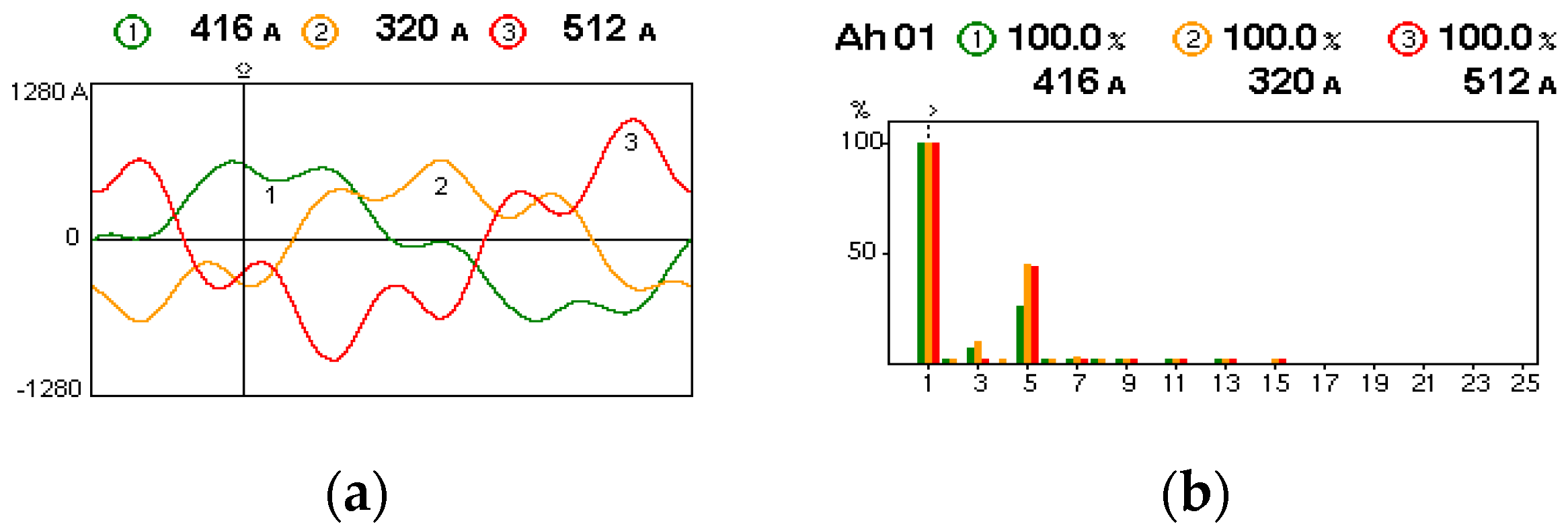
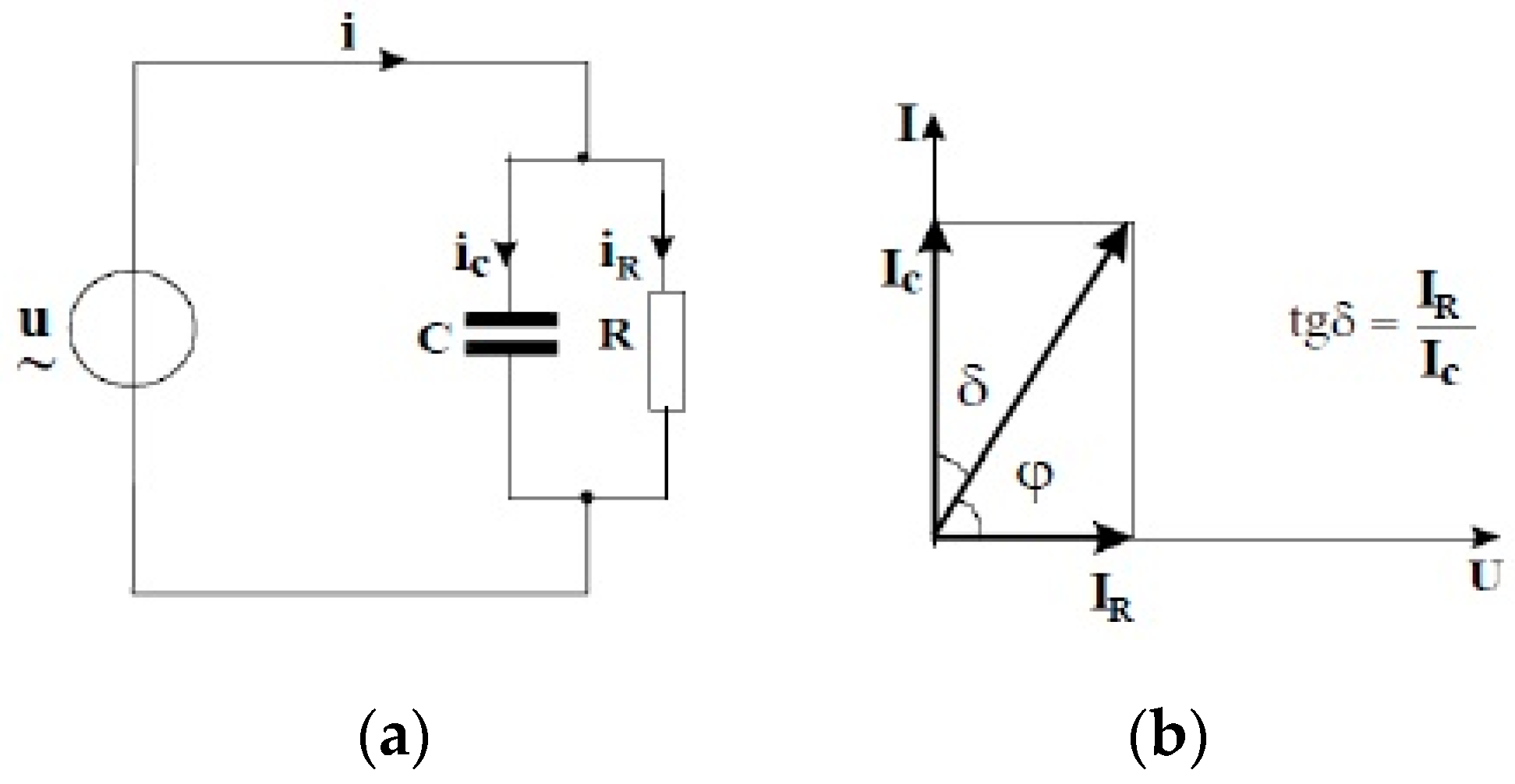
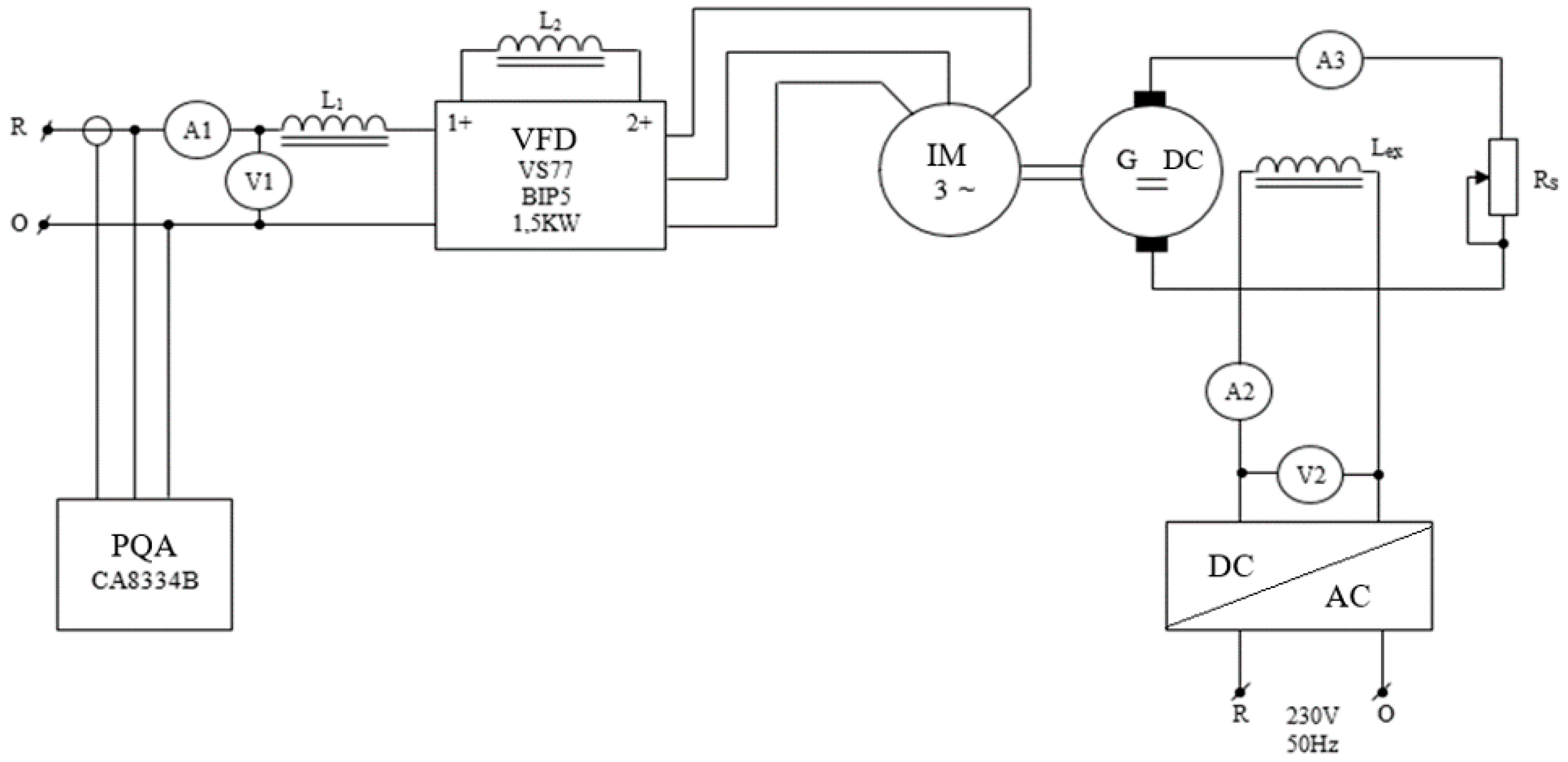
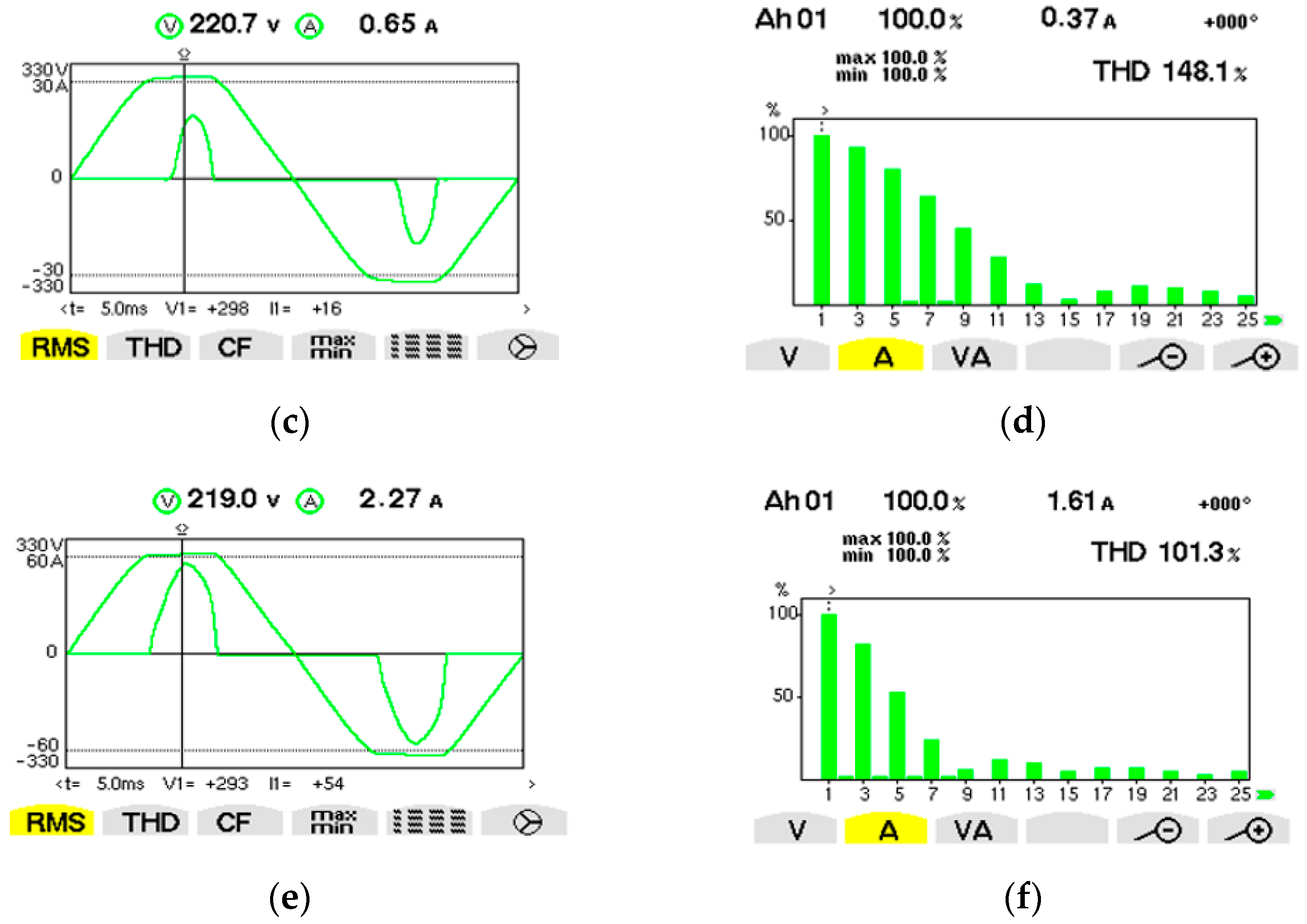
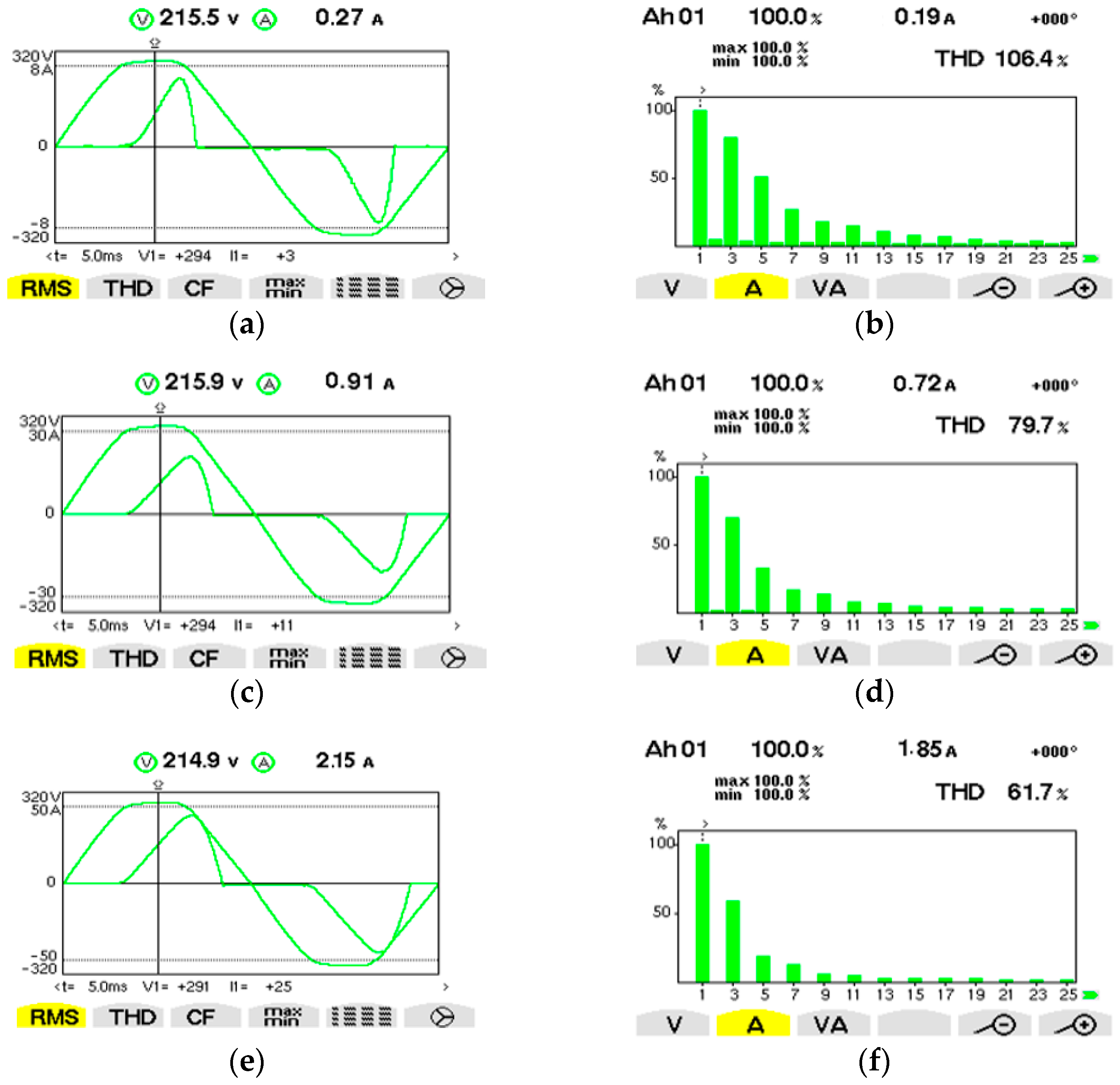
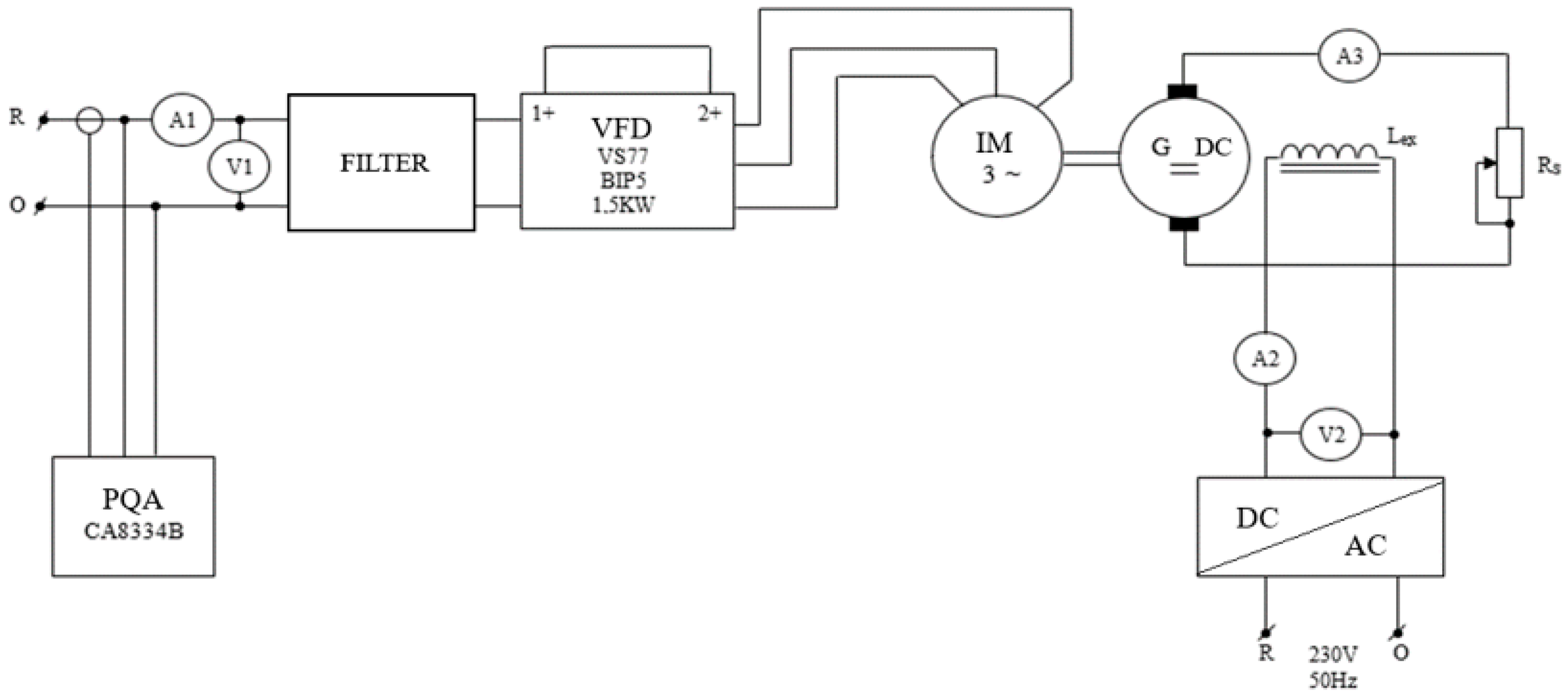
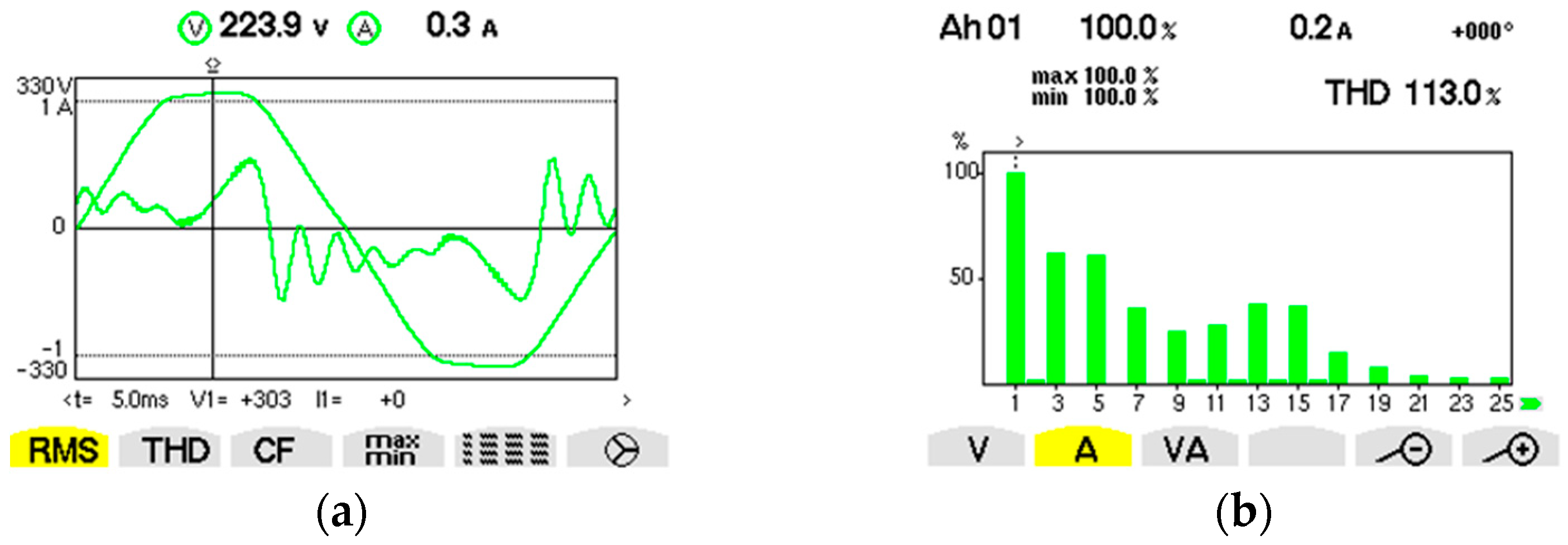
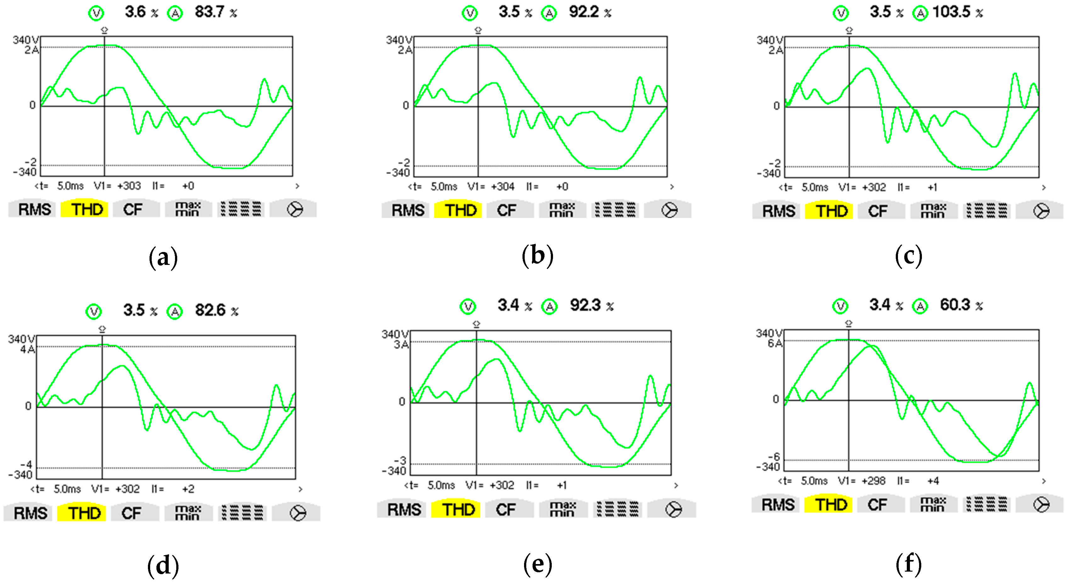
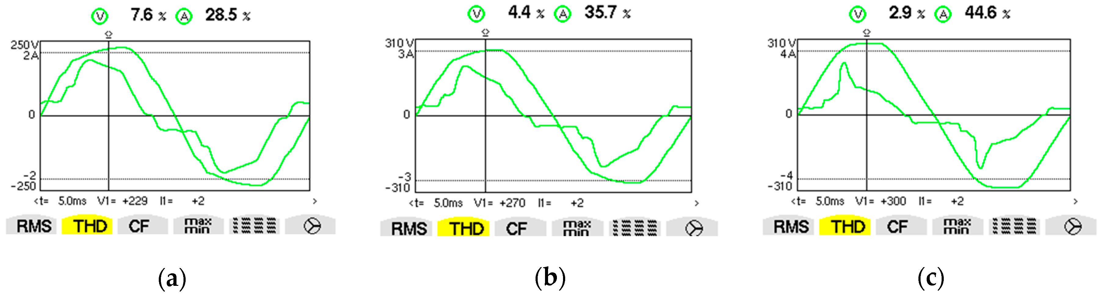
Table 1.
Experimental measurements for an AC coreless coil.
| fm (kHz) | L (mH) | Q (−) | φ (°) | tanδ (−) |
|---|---|---|---|---|
| 0.1 | 47.1 | 3.97 | 75.9 | 0.251 |
| 0.12 | 47.1 | 4.77 | 78.1 | 0.209 |
| 1 | 47.27 | 35.5 | 88.3 | 0.028 |
| 10 | 97.74 | 25.6 | 87.7 | 0.039 |
Table 2.
Experimental measurements for an AC ferromagnetic core coil.
| fm (kHz) | L (mH) | Q (−) | φ (°) | tanδ (−) |
|---|---|---|---|---|
| 0.1 | 98.86 | 3.8 | 75.3 | 0.262 |
| 0.12 | 95.2 | 3.95 | 75.8 | 0.252 |
| 1 | 71.35 | 3.73 | 71.33 | 0.267 |
| 10 | 33.72 | 0.589 | 30.5 | 1.69 |
Table 3.
Experimental measurements for an old AC capacitor (more than 3000 h of operation).
| fm (kHz) | C (µF) | Q (−) | φ (°) | tanδ (−) |
|---|---|---|---|---|
| 0.1 | 2.235 | 96.2 | 89.4 | 0.01 |
| 0.12 | 2.248 | 96.5 | 89.4 | 0.01 |
| 1 | 2.222 | 65.4 | 89.1 | 0.015 |
| 10 | 2.175 | 21.4 | 87.3 | 0.46 |
Table 4.
Experimental measurements for a new AC capacitor.
| fm (kHz) | C (µF) | Q (−) | φ (°) | tanδ (−) |
|---|---|---|---|---|
| 0.1 | 1.8467 | 370 | 89.8 | 0.002 |
| 0.12 | 1.8474 | 249 | 89.6 | 0.004 |
| 1 | 1.8475 | 490 | 89.8 | 0.002 |
| 10 | 1.8552 | 204 | 89.7 | 0.005 |
Table 5.
Experimental measurements made with the motor at idle (Rs not connected), L1 and L2 short-circuited (Figure 5).
Table 5.
Experimental measurements made with the motor at idle (Rs not connected), L1 and L2 short-circuited (Figure 5).
| fvfd (Hz) | Is (A) | THDc (%) |
|---|---|---|
| 10 | 0.26 | 103.7 |
| 30 | 0.32 | 100 |
| 50 | 0.37 | 96.9 |
Table 6.
Experimental measurements made with L1 and L2 short-circuited (Figure 5).
Table 6.
Experimental measurements made with L1 and L2 short-circuited (Figure 5).
| fvfd (Hz) | Rs (Ω) | Ir (A) | Is (A) | THDc (%) | P (W) | Q (W) | S (VA) | PF (−) | DPF (−) |
|---|---|---|---|---|---|---|---|---|---|
| 10 | 4.2 | 0.25 | 0.19 | 169.7 | 30.79 | 54.5 | 63.27 | 0.488 | 0.986 |
| 10 | 2.4 | 0.44 | 0.2 | 170 | 31.4 | 55.5 | 63.9 | 0.49 | 0.986 |
| 10 | 0.7 | 1.45 | 0.23 | 168.4 | 34.5 | 61.3 | 70.3 | 0.492 | 0.986 |
| 30 | 4.2 | 1.25 | 0.43 | 149.9 | 70.1 | 110.7 | 131.4 | 0.535 | 0.989 |
| 30 | 2.4 | 2.14 | 0.51 | 147 | 79.9 | 122.7 | 146.9 | 0.546 | 0.99 |
| 30 | 0.7 | 6.04 | 0.91 | 133.1 | 132.5 | 183.8 | 229 | 0.589 | 0.993 |
| 50 | 4.2 | 2.31 | 0.83 | 133.1 | 129.5 | 180.1 | 223.5 | 0.584 | 0.993 |
| 50 | 2.4 | 3.82 | 1.06 | 125.1 | 170.9 | 223.1 | 280.8 | 0.61 | 0.994 |
| 50 | 0.7 | 9.41 | 2.19 | 102.7 | 331.5 | 359 | 490.9 | 0.683 | 0.999 |
Table 7.
Experimental measurements made with a DC filter, inductance coil L1 = 20 mH, Rl = 1.6 Ω, and L2 short-circuited (Figure 5).
Table 7.
Experimental measurements made with a DC filter, inductance coil L1 = 20 mH, Rl = 1.6 Ω, and L2 short-circuited (Figure 5).
| fvfd (Hz) | Rs (Ω) | Ir (A) | Is (A) | THDc (%) | P (W) | Q (W) | S (VA) | PF (−) | DPF (−) |
|---|---|---|---|---|---|---|---|---|---|
| 10 | 4.2 | 0.22 | 0.21 | 106.3 | 30.68 | 34.5 | 46 | 0.661 | 0.963 |
| 10 | 2.4 | 0.4 | 0.22 | 106.9 | 31.2 | 34.9 | 47 | 0.667 | 0.963 |
| 10 | 0.7 | 1.09 | 0.25 | 104.7 | 35.8 | 39.6 | 53.6 | 0.669 | 0.96 |
| 30 | 4.2 | 0.76 | 0.43 | 92.9 | 65.4 | 65.5 | 92.8 | 0.707 | 0.955 |
| 30 | 2.4 | 1.41 | 0.48 | 90.5 | 76.2 | 74.4 | 107.7 | 0.716 | 0.954 |
| 30 | 0.7 | 5.4 | 0.88 | 77.7 | 145.3 | 128.9 | 195.7 | 0.752 | 0.945 |
| 50 | 4.2 | 2.02 | 0.86 | 79.1 | 136.7 | 121.7 | 184.1 | 0.748 | 0.945 |
| 50 | 2.4 | 3.38 | 1.08 | 74.2 | 179.1 | 153.6 | 237.2 | 0.761 | 0.94 |
| 50 | 0.7 | 8.94 | 2.17 | 59 | 377.1 | 290.9 | 478.4 | 0.792 | 0.918 |
Table 8.
Experimental measurements made with a filter on AC, inductance coil L1 = 20 mH, Rl = 1.6 Ω, and L2 short-circuited (Figure 5).
Table 8.
Experimental measurements made with a filter on AC, inductance coil L1 = 20 mH, Rl = 1.6 Ω, and L2 short-circuited (Figure 5).
| fvfd (Hz) | Rs (Ω) | Ir (A) | Is (A) | THDc (%) | P (W) | Q (W) | S (VA) | PF (−) | DPF (−) |
|---|---|---|---|---|---|---|---|---|---|
| 10 | 4.2 | 0.4 | 0.22 | 112 | 30.7 | 36 | 45.5 | 0.645 | 0.946 |
| 10 | 2.4 | 0.63 | 0.23 | 110 | 32 | 36.4 | 48.2 | 0.659 | 0.958 |
| 10 | 0.7 | 1.9 | 0.27 | 103.3 | 40 | 44.6 | 59.6 | 0.674 | 0.958 |
| 30 | 4.2 | 1.3 | 0.49 | 92.9 | 73.9 | 73.5 | 104 | 0.71 | 0.954 |
| 30 | 2.4 | 2.22 | 0.55 | 89.8 | 85.5 | 83.5 | 119.4 | 0.716 | 0.953 |
| 30 | 0.7 | 6.05 | 0.93 | 78.3 | 152.1 | 135.7 | 204.7 | 0.747 | 0.946 |
| 50 | 4.2 | 2.22 | 0.86 | 80.9 | 138.2 | 124.9 | 186.4 | 0.742 | 0.947 |
| 50 | 2.4 | 3.87 | 1.1 | 76.1 | 182 | 157.9 | 241.9 | 0.757 | 0.942 |
| 50 | 0.7 | 9.4 | 2.22 | 61.2 | 376.6 | 294.2 | 478.5 | 0.788 | 0.922 |
Table 9.
Experimental measurements made with coils on AC and DC, L1 = L2 = 20 mH, and Rl = 1.6 Ω (Figure 5).
Table 9.
Experimental measurements made with coils on AC and DC, L1 = L2 = 20 mH, and Rl = 1.6 Ω (Figure 5).
| fvfd (Hz) | Rs (Ω) | Ir (A) | Is (A) | THDc (%) | P (W) | Q (W) | S (VA) | PF (−) | DPF (−) |
|---|---|---|---|---|---|---|---|---|---|
| 10 | 4.2 | 0.25 | 0.19 | 96.6 | 29.15 | 30 | 41.7 | 0.695 | 0.957 |
| 10 | 2.4 | 0.44 | 0.2 | 95.8 | 30 | 31 | 43 | 0.698 | 0.957 |
| 10 | 0.7 | 1.45 | 0.23 | 92.5 | 35.9 | 35.95 | 50.97 | 0.71 | 0.955 |
| 30 | 4.2 | 1.25 | 0.43 | 80.7 | 70.4 | 63.9 | 95.8 | 0.741 | 0.945 |
| 30 | 2.4 | 2.14 | 0.51 | 77.5 | 84.4 | 74.4 | 112.7 | 0.75 | 0.941 |
| 30 | 0.7 | 6.04 | 0.91 | 65.8 | 154.9 | 126.2 | 201.3 | 0.777 | 0.925 |
| 50 | 4.2 | 2.31 | 0.83 | 67.9 | 138.9 | 114.8 | 180 | 0.77 | 0.927 |
| 50 | 2.4 | 3.82 | 1.06 | 62.3 | 182.9 | 146.3 | 235.1 | 0.784 | 0.916 |
| 50 | 0.7 | 9.41 | 2.19 | 45.4 | 376.9 | 287.1 | 474.8 | 0.797 | 0.897 |
Table 10.
Experimental measurements made with an LC filter, L = 20 mH, C = 2 µF, fc = 795.8 Hz (Figure 10).
Table 10.
Experimental measurements made with an LC filter, L = 20 mH, C = 2 µF, fc = 795.8 Hz (Figure 10).
| fvfd (Hz) | Rs (Ω) | Ir (A) | Is (A) | THDc (%) | P (W) | Q (W) | S (VA) | PF (−) | DPF (−) |
|---|---|---|---|---|---|---|---|---|---|
| 10 | 4.2 | 0.11 | 0.440 | 113.3 | 30.4 | 54.3 | 63.8 | 0.476 | 0.726 |
| 10 | 2.4 | 0.2 | 0.406 | 114.7 | 31 | 54.9 | 63.5 | 0.475 | 0.738 |
| 10 | 0.7 | 0.61 | 0.387 | 114.1 | 33.1 | 55.8 | 64.5 | 0.481 | 0.753 |
| 30 | 4.2 | 0.47 | 0.576 | 110.1 | 64.1 | 75.5 | 103.1 | 0.61 | 0.956 |
| 30 | 2.4 | 0.87 | 0.6 | 109.3 | 69.3 | 79.3 | 110.6 | 0.623 | 0.969 |
| 30 | 0.7 | 2.91 | 0.791 | 99.7 | 104.9 | 103.8 | 159.9 | 0.684 | 0.998 |
| 50 | 4.2 | 0.85 | 0.838 | 97.8 | 114.2 | 110.5 | 165.9 | 0.686 | 0.999 |
| 50 | 2.4 | 1.67 | 0.975 | 94.7 | 141.8 | 132.5 | 189.6 | 0.703 | 1 |
| 50 | 0.7 | 6.93 | 1.977 | 69.7 | 336.6 | 253.5 | 439 | 0.765 | 0.979 |
Table 11.
Experimental measurements made with an LC filter, L = 20 mH, C = 2 µF (Figure 10).
Table 11.
Experimental measurements made with an LC filter, L = 20 mH, C = 2 µF (Figure 10).
| fvfd (Hz) | Rs (Ω) | Ir (A) | Is (A) | THDc (%) | P (W) | Q (W) | S (VA) | PF (−) | DPF (−) |
|---|---|---|---|---|---|---|---|---|---|
| 10 | 4.2 | 0.18 | 0.658 | 95 | 29.79 | 46.24 | 54.65 | 0.54 | 0.734 |
| 10 | 2.4 | 0.26 | 0.706 | 96 | 30 | 46.45 | 55.18 | 0.543 | 0.74 |
| 10 | 0.7 | 0.71 | 0.776 | 97.4 | 32.36 | 47.61 | 57.8 | 0.563 | 0.776 |
| 30 | 4.2 | 0.54 | 1.275 | 100.7 | 63.56 | 66.57 | 92.15 | 0.491 | 0.971 |
| 30 | 2.4 | 0.99 | 1.453 | 100.1 | 70.6 | 71.6 | 100.2 | 0.701 | 0.982 |
| 30 | 0.7 | 3.35 | 0.639 | 90 | 118.5 | 104.5 | 159.8 | 0.756 | 0.999 |
| 50 | 4.2 | 1.12 | 0.659 | 89.7 | 117.4 | 102.6 | 156.8 | 0.754 | 1 |
| 50 | 2.4 | 2.31 | 0.809 | 83 | 141.8 | 129 | 204.9 | 0.772 | 0.992 |
| 50 | 0.7 | 8.41 | 1.781 | 64.6 | 336.6 | 261.5 | 442 | 0.805 | 0.954 |
Table 12.
The LC filter parameters used in the experiments.
| L (mH) | C (µF) | fres (Hz) | |
|---|---|---|---|
| LC Filter 1 | 77.7 | 6.5 | 224 |
| LC Filter 2 | 95.43 | 10 | 162.92 |
| LC Filter 3 | 95.43 | 5 | 230.4 |
| LC Filter 4 | 95.43 | 3.5 | 275.38 |
Table 13.
Experimental measurements with FVD + IM, without and with filters, at fvfd 10 Hz (Figure 10).
Table 13.
Experimental measurements with FVD + IM, without and with filters, at fvfd 10 Hz (Figure 10).
| THDc (%) | P (W) | Q (VAR) | S (VA) | PF (−) | DPF (−) | |
|---|---|---|---|---|---|---|
| No Filter | 159.3 | 39.4 | 67.3 | 78.4 | 0.506 | 0.987 |
| LC Filter 1 | 51.95 | 43.9 | 125.7 | 133.4 | 0.329 | 0.372 |
| LC Filter 2 | 33.05 | 48.9 | 181 | 187.8 | 0.26 | 0.276 |
| LC Filter 3 | 64.15 | 42.2 | 94.9 | 103.5 | 0.406 | 0.483 |
| LC Filter 4 | 106.15 | 42 | 84.5 | 95 | 0.44 | 0.612 |
Table 14.
Experimental measurements with FVD + IM, without and with filters, at fvfd 30 Hz (Figure 10).
Table 14.
Experimental measurements with FVD + IM, without and with filters, at fvfd 30 Hz (Figure 10).
| THDc (%) | P (W) | Q (VAR) | S (VA) | PF (−) | DPF (−) | |
|---|---|---|---|---|---|---|
| No Filter | 158.15 | 51.2 | 84.8 | 98.9 | 0.521 | 0.987 |
| LC Filter 1 | 65.70 | 56 | 133 | 144.5 | 0.385 | 0.463 |
| LC Filter 2 | 41.40 | 61.1 | 184.3 | 193.7 | 0.312 | 0.34 |
| LC Filter 3 | 77.25 | 54.5 | 104 | 117.5 | 0.462 | 0.584 |
| LC Filter 4 | 106.50 | 53 | 93.2 | 104.5 | 0.491 | 0.724 |
Table 15.
Experimental measurements with FVD + IM, without and with filters, at fvfd 50 Hz (Figure 10).
Table 15.
Experimental measurements with FVD + IM, without and with filters, at fvfd 50 Hz (Figure 10).
| THDc (%) | P (W) | Q (VAR) | S (VA) | PF (−) | DPF (−) | |
|---|---|---|---|---|---|---|
| No Filter | 146.35 | 64.4 | 98.1 | 117.6 | 0.543 | 0.989 |
| LC Filter 1 | 74.90 | 66.8 | 142.2 | 156.9 | 0.423 | 0.532 |
| LC Filter 2 | 50.45 | 73.5 | 190.4 | 204.9 | 0.361 | 0.408 |
| LC Filter 3 | 84.25 | 65.7 | 110.1 | 128.1 | 0.515 | 0.673 |
| LC Filter 4 | 113 | 62.1 | 102.1 | 120.1 | 0.513 | 0.78 |
Table 16.
Experimental measurements made with the T filter, L1 = L2 = 20 mH, C = 2 μF, fres = 1.125 kHz (Figure 10).
Table 16.
Experimental measurements made with the T filter, L1 = L2 = 20 mH, C = 2 μF, fres = 1.125 kHz (Figure 10).
| fvfd (Hz) | Rs (Ω) | Ir (A) | Is (A) | THDc (%) | P (W) | Q (W) | S (VA) | PF (−) |
|---|---|---|---|---|---|---|---|---|
| 10 | 4.2 | 0.65 | 0.272 | 101.7 | 47.4 | 53.6 c | 71.4 | 0.663 |
| 10 | 2.4 | 1.27 | 0.278 | 101.5 | 49.1 | 54.6 c | 73.3 | 0.668 |
| 10 | 0.7 | 3.6 | 0.315 | 98.9 | 57.5 | 59.1 c | 82.3 | 0.697 |
| 30 | 4.2 | 2.4 | 0.537 | 87.1 | 100.2 | 85.6 i | 131.7 | 0.76 |
| 30 | 2.4 | 4.3 | 0.66 | 81.7 | 123.6 | 101.6 i | 159.8 | 0.772 |
| 30 | 0.7 | 13 | 1.289 | 61.2 | 242.8 | 174.7 i | 298.7 | 0.81 |
| 50 | 4.2 | 4 | 0.941 | 69.2 | 178.3 | 133.2 i | 222.3 | 0.8 |
| 50 | 2.4 | 6.7 | 1.261 | 61.6 | 238.2 | 172.1 i | 293.9 | 0.811 |
| 50 | 0.7 | 13.8 | 2.56 | 42.3 | 466.8 | 334.1 i | 573.9 | 0.813 |
Table 17.
Experimental measurements made with the T filter, L1 = L2 = 20 mH, C = 5 μF, fres = 711.76 Hz (Figure 10).
Table 17.
Experimental measurements made with the T filter, L1 = L2 = 20 mH, C = 5 μF, fres = 711.76 Hz (Figure 10).
| fvfd (Hz) | Rs (Ω) | Ir (A) | Is (A) | THDc (%) | P (W) | Q (W) | S (VA) | PF (−) |
|---|---|---|---|---|---|---|---|---|
| 10 | 4.2 | 0.6 | 0.413 | 85.3 | 47.8 | 93.3 c | 105 | 0.456 |
| 10 | 2.4 | 1.2 | 0.417 | 86.2 | 49.5 | 93.5 c | 106 | 0.466 |
| 10 | 0.7 | 3.8 | 0.442 | 90 | 58.6 | 96.4 c | 112.7 | 0.52 |
| 30 | 4.2 | 2.5 | 0.588 | 91.7 | 100.6 | 109.4 c | 148.7 | 0.677 |
| 30 | 2.4 | 4.3 | 0.681 | 88.6 | 123.4 | 117.5 c | 170.3 | 0.725 |
| 30 | 0.7 | 13.6 | 1.303 | 73.2 | 248.2 | 187.3 i | 309.3 | 0.798 |
| 50 | 4.2 | 4 | 0.926 | 81 | 177.4 | 141.9 c | 227.2 | 0.78 |
| 50 | 2.4 | 6.6 | 1.226 | 74.4 | 235.8 | 187.7 i | 296 | 0.796 |
| 50 | 0.7 | 14.4 | 2.52 | 46.2 | 481.7 | 310.8 i | 574.1 | 0.84 |
Table 18.
Experimental measurements made with the T filter, L1 = L2 = 11.5 mH, C = 5 μF, fres = 938.64 Hz (Figure 10).
Table 18.
Experimental measurements made with the T filter, L1 = L2 = 11.5 mH, C = 5 μF, fres = 938.64 Hz (Figure 10).
| fvfd (Hz) | Rs (Ω) | Ir (A) | Is (A) | THDc (%) | P (W) | Q (W) | S (VA) | PF (−) |
|---|---|---|---|---|---|---|---|---|
| 10 | 4.2 | 0.4 | 0.413 | 83.2 | 47.1 | 94.4 c | 105.6 | 0.445 |
| 10 | 2.4 | 0.8 | 0.419 | 85.9 | 49.1 | 95.7 c | 107.5 | 0.457 |
| 10 | 0.7 | 3.1 | 0.447 | 92.7 | 58.7 | 100.2 c | 115.8 | 0.503 |
| 30 | 4.2 | 2 | 0.6 | 104.3 | 97.9 | 120.5 c | 155.4 | 0.63 |
| 30 | 2.4 | 4.2 | 0.698 | 103.4 | 120.7 | 133.7 c | 179.8 | 0.669 |
| 30 | 0.7 | 12.8 | 1.244 | 82.5 | 236.3 | 192.6 i | 306.2 | 0.776 |
| 50 | 4.2 | 4.1 | 0.954 | 92.3 | 178 | 162.8 c | 240.9 | 0.738 |
| 50 | 2.4 | 6.9 | 1.246 | 82.5 | 236.8 | 192.4 i | 305.2 | 0.775 |
| 50 | 0.7 | 16.6 | 2.81 | 60.2 | 527.9 | 369.8 i | 641.8 | 0.819 |
Table 19.
Experimental measurements made with the T filter, L1 = L2 = 11.5 mH, C = 2 μF, fres = 1.484 kHz (Figure 10).
Table 19.
Experimental measurements made with the T filter, L1 = L2 = 11.5 mH, C = 2 μF, fres = 1.484 kHz (Figure 10).
| fvfd (Hz) | Rs (Ω) | Ir (A) | Is (A) | THDc (%) | P (W) | Q (W) | S (VA) | PF (−) |
|---|---|---|---|---|---|---|---|---|
| 10 | 4.2 | 0.8 | 0.278 | 107.4 | 46.8 | 57.1 c | 74.4 | 0.633 |
| 10 | 2.4 | 1.2 | 0.29 | 107.2 | 49.1 | 58.8 c | 76.7 | 0.642 |
| 10 | 0.7 | 3.6 | 0.346 | 106.5 | 60.6 | 67.1 c | 90.5 | 0.67 |
| 30 | 4.2 | 2.4 | 0.539 | 97.7 | 97 | 93.6 c | 134.7 | 0.72 |
| 30 | 2.4 | 4.2 | 0.656 | 92.7 | 119 | 109.5 i | 161.6 | 0.736 |
| 30 | 0.7 | 12.7 | 1.26 | 75.3 | 234 | 187.3 i | 299.2 | 0.78 |
| 50 | 4.2 | 4 | 0.949 | 83.6 | 175.3 | 150 i | 230.5 | 0.76 |
| 50 | 2.4 | 7 | 1.289 | 74.6 | 240.4 | 191.5 i | 306.5 | 0.782 |
| 50 | 0.7 | 16.1 | 2.74 | 56.1 | 505.1 | 363.5 i | 628.1 | 0.814 |
Table 20.
Three lamps supplied with variable voltage (R = 0 Ω, Figure 19).
Table 20.
Three lamps supplied with variable voltage (R = 0 Ω, Figure 19).
| Us (V) | Is (A) | THDu (%) | THDc (%) | PF (−) | DPF (−) |
|---|---|---|---|---|---|
| 130.4 | 0.978 | 3.6 | 65.3 | 0.812 | 0.971 |
| 150.7 | 0.957 | 3.3 | 62.9 | 0.833 | 0.976 |
| 175.2 | 1.049 | 3.3 | 54.9 | 0.872 | 0.986 |
| 200.7 | 1.154 | 3.4 | 51.2 | 0.886 | 0.99 |
| 220.6 | 1.139 | 3.4 | 48.4 | 0.895 | 0.99 |
Table 21.
Three lamps powered at variable voltage by variable R, without filters (Figure 19).
Table 21.
Three lamps powered at variable voltage by variable R, without filters (Figure 19).
| Us (V) | Is (A) | THDu (%) | THDc (%) | PF (−) | DPF (−) |
|---|---|---|---|---|---|
| 134 | 0.871 | 14.8 | 23.9 | 0.917 | 0.992 |
| 150.1 | 0.859 | 11.9 | 26.5 | 0.925 | 0.993 |
| 174.8 | 0.948 | 8 | 31.6 | 0.928 | 0.994 |
| 200 | 1.14 | 4.6 | 39.2 | 0.92 | 0.995 |
| 219.6 | 1.145 | 2.9 | 48.8 | 0.904 | 0.991 |
Table 22.
Three lamps powered at variable voltage through variable R, LC shunt filter, L = 43 mH, C = 2 μF, fres = 542.71 Hz (Figure 19).
Table 22.
Three lamps powered at variable voltage through variable R, LC shunt filter, L = 43 mH, C = 2 μF, fres = 542.71 Hz (Figure 19).
| Us (V) | Is (A) | THDu (%) | THDc (%) |
|---|---|---|---|
| 129.5 | 0.914 | 14.7 | 21.6 |
| 151.8 | 0.895 | 11.4 | 25.3 |
| 175.4 | 0.989 | 7.9 | 30.7 |
| 200 | 1.175 | 4.4 | 38.1 |
| 219.1 | 1.194 | 2.9 | 47.6 |
Table 23.
Three lamps powered at variable voltage through variable R, LC shunt filter, L = 8.82 mH, C = 2 μF, fres = 1.198 kHz (Figure 2).
Table 23.
Three lamps powered at variable voltage through variable R, LC shunt filter, L = 8.82 mH, C = 2 μF, fres = 1.198 kHz (Figure 2).
| Us (V) | Is (A) | THDu (%) | THDc (%) |
|---|---|---|---|
| 126.2 | 0.976 | 16.1 | 22.9 |
| 150 | 0.945 | 11.7 | 25.5 |
| 174.9 | 1.023 | 7.8 | 31.1 |
| 199.6 | 1.2 | 4.5 | 37.5 |
| 220 | 1.218 | 2.8 | 47.7 |
Table 24.
Three lamps powered at variable voltage through variable R, LC shunt filter, L = 8.82 mH, C = 2 μF (Figure 19).
Table 24.
Three lamps powered at variable voltage through variable R, LC shunt filter, L = 8.82 mH, C = 2 μF (Figure 19).
| Us (V) | Is (A) | THDu (%) | THDc (%) |
|---|---|---|---|
| 124.3 | 1.008 | 15.8 | 20.8 |
| 150.2 | 0.978 | 11.4 | 23.7 |
| 175.5 | 1.061 | 7.6 | 28.5 |
| 200.8 | 1.214 | 4.4 | 35.7 |
| 220 | 1.237 | 3 | 44.8 |
Table 25.
Three lamps powered at variable voltage through variable R, LCL filter L1 = L2 = 43 mH, C = 4 μF, fres = 383.75 Hz (Figure 19).
Table 25.
Three lamps powered at variable voltage through variable R, LCL filter L1 = L2 = 43 mH, C = 4 μF, fres = 383.75 Hz (Figure 19).
| Us (V) | Is (A) | THDu (%) | THDc (%) |
|---|---|---|---|
| 128.9 | 0.957 | 15.2 | 19.7 |
| 150.1 | 0.967 | 11.7 | 22.7 |
| 175.4 | 0.979 | 7.9 | 28.2 |
| 200.2 | 1.104 | 4.4 | 35.2 |
| 219.9 | 1.216 | 3.1 | 40.4 |
Table 26.
Three lamps powered at variable voltage through variable R, LCL filter, L1 = L2 = 43 mH, C = 2 μF, fres = 767.51 Hz (Figure 19).
Table 26.
Three lamps powered at variable voltage through variable R, LCL filter, L1 = L2 = 43 mH, C = 2 μF, fres = 767.51 Hz (Figure 19).
| Us (V) | Is (A) | THDu (%) | THDc (%) |
|---|---|---|---|
| 132.1 | 0.957 | 15.3 | 21.5 |
| 150 | 0.941 | 12.1 | 24.4 |
| 174.9 | 0.947 | 7.7 | 28.6 |
| 199.9 | 1.079 | 4.1 | 32 |
| 220.2 | 1.189 | 3 | 34.8 |
Table 27.
Average values determined from the experimental measurements in Section 4.1.
Table 27.
Average values determined from the experimental measurements in Section 4.1.
| No. | Section | THDc (%) | P (W) | Q (W) | S (VA) | PF (−) |
|---|---|---|---|---|---|---|
| 1 | Section 4.1.1 | 144.33 | 112.34 | 150.11 | 188.88 | 0.557 |
| 2 | Section 4.1.2 | 87.92 | 119.72 | 104.88 | 160.27 | 0.719 |
| 3 | Section 4.1.3 | 89.38 | 123.44 | 109.63 | 165.35 | 0.715 |
| 4 | Section 4.1.4 | 76.05 | 122.6 | 101.07 | 159.48 | 0.746 |
| 5 | Section 4.1.5 | 102.6 | 102.82 | 102.23 | 151.1 | 0.611 |
| 6 | Section 4.1.6 | 90.722 | 104.51 | 97.34 | 147.05 | 0.658 |
| 7 | Section 4.1.8 | 78.35 | 167.1 | 129.84 | 211.92 | 0.754 |
| 8 | Section 4.1.9 | 79.62 | 169.22 | 129.86 | 227.7 | 0.673 |
| 9 | Section 4.1.10 | 87.44 | 172.5 | 162.45 | 239.8 | 0.645 |
| 10 | Section 4.1.11 | 89.01 | 169.7 | 142.04 | 222.47 | 0.726 |
Table 28.
Reduction of greenhouse gas emissions when using passive filters.
| No. | Section | Year | Region | CO2e (g/kWh) | Percentage Reduction of Active Energy (%) | Reduction CO2e (g/kWh) | Reduction CO2 (g/kWh) |
|---|---|---|---|---|---|---|---|
| 1 | Section 4.1.5 | 2022 | Ro, EU | 245 | 8.47 | 20.75 | 16.6 |
| 2 | Section 4.1.6 | 2022 | Ro, EU | 245 | 7 | 17.15 | 13.72 |
| 3 | Section 4.1.5 | 2024 | Ro | 210 | 8.47 | 17.787 | |
| 4 | Section 4.1.6 | 2024 | Ro | 210 | 7 | 14.7 | |
| 5 | Section 4.1.5 | 2024 | EU | 235 | 8.47 | 19.904 | |
| 6 | Section 4.1.6 | 2024 | EU | 235 | 7 | 16.45 | |
| 7 | Section 4.1.5 | 2030 | EU | 96 | 8.47 | 8.13 | |
| 8 | Section 4.1.6 | 2030 | EU | 96 | 7 | 6.72 |
Table 29.
Reduction of losses of active power and active electrical energy on the line for the cases analyzed in Section 4.1.
Table 29.
Reduction of losses of active power and active electrical energy on the line for the cases analyzed in Section 4.1.
| No. | Section | PFf (−) | ΔPl (%) | ΔWl (%) |
|---|---|---|---|---|
| 1 | Section 4.1.2 | 0.719 | 40 | 40 |
| 2 | Section 4.1.3 | 0.715 | 39.31 | 39.31 |
| 3 | Section 4.1.4 | 0.746 | 44.25 | 44.25 |
| 4 | Section 4.1.5 | 0.611 | 16.89 | 16.89 |
| 5 | Section 4.1.6 | 0.658 | 28.34 | 28.34 |
| 6 | Section 4.1.8 | 0.754 | 45.42 | 45.42 |
| 7 | Section 4.1.9 | 0.673 | 31.5 | 31.5 |
| 8 | Section 4.1.10 | 0.645 | 25.42 | 25.42 |
| 9 | Section 4.1.11 | 0.726 | 41.13 | 41.13 |
Table 30.
Reduction of active power losses on the line for the case R = 1.5 Ω, I = 2.17 A, t = 1000 h.
Table 30.
Reduction of active power losses on the line for the case R = 1.5 Ω, I = 2.17 A, t = 1000 h.
| No. | Section | ΔWl (%) | Reduction CO2e (g/kWh) | Reduction CO2 (g/kWh) |
|---|---|---|---|---|
| 1 | Section 4.1.2 | 40 | 2.08 | 1.66 |
| 2 | Section 4.1.3 | 39.31 | 2.04 | 1.63 |
| 3 | Section 4.1.4 | 44.25 | 2.3 | 1.83 |
| 4 | Section 4.1.5 | 16.89 | 0.88 | 0.7 |
| 5 | Section 4.1.6 | 28.34 | 1.47 | 1.17 |
| 6 | Section 4.1.8 | 45.42 | 2.36 | 1.89 |
| 7 | Section 4.1.9 | 31.5 | 1.63 | 1.31 |
| 8 | Section 4.1.10 | 25.42 | 1.32 | 1.06 |
| 9 | Section 4.1.11 | 41.13 | 2.13 | 1.71 |
Disclaimer/Publisher’s Note: The statements, opinions and data contained in all publications are solely those of the individual author(s) and contributor(s) and not of MDPI and/or the editor(s). MDPI and/or the editor(s) disclaim responsibility for any injury to people or property resulting from any ideas, methods, instructions or products referred to in the content. |
© 2024 by the authors. Licensee MDPI, Basel, Switzerland. This article is an open access article distributed under the terms and conditions of the Creative Commons Attribution (CC BY) license (https://creativecommons.org/licenses/by/4.0/).
Share and Cite
MDPI and ACS Style
Diniș, C.M.; Popa, G.N.; Cunțan, C.D.; Iagăr, A. Aspects Regarding of Passive Filters Sustainability for Non-Linear Single-Phase Consumers. Sustainability 2024, 16, 2776. https://0-doi-org.brum.beds.ac.uk/10.3390/su16072776
AMA Style
Diniș CM, Popa GN, Cunțan CD, Iagăr A. Aspects Regarding of Passive Filters Sustainability for Non-Linear Single-Phase Consumers. Sustainability. 2024; 16(7):2776. https://0-doi-org.brum.beds.ac.uk/10.3390/su16072776
Chicago/Turabian StyleDiniș, Corina Maria, Gabriel Nicolae Popa, Corina Daniela Cunțan, and Angela Iagăr. 2024. "Aspects Regarding of Passive Filters Sustainability for Non-Linear Single-Phase Consumers" Sustainability 16, no. 7: 2776. https://0-doi-org.brum.beds.ac.uk/10.3390/su16072776
Note that from the first issue of 2016, this journal uses article numbers instead of page numbers. See further details here.