Article

Environmental Regulation, Economic Network and Sustainable Growth of Urban Agglomerations in China

1
School of Economics, Jinan University, Guangzhou 510632, China
2
Department of Geography, Kent State University, Kent, OH 44242, USA
*
Author to whom correspondence should be addressed.
Sustainability 2016, 8(5), 467; https://0-doi-org.brum.beds.ac.uk/10.3390/su8050467
Submission received: 25 December 2015 / Revised: 4 May 2016 / Accepted: 5 May 2016 / Published: 11 May 2016

Abstract

:
In this paper, we examine the influence of environmental regulation on sustainable economic growth from both theoretical and empirical perspectives. Our research is twofold. First, we apply a modified NEG (New Economic Geography) model to analyze how environmental regulation influences firms’ location choices and cities’ sustainable economic growth. Second, we test a spatial econometric model employing panel data of the three largest urban agglomerations in China from 2003 to 2013 to study the relationship between environmental regulation and sustainable economic growth as well as the spillover channels of economic activities. The results reveal a remarkable negative effect of environmental regulation on economic growth. In addition, we find no sufficient evidence to prove the existence of long-term effects of environmental regulation on economic growth in the three urban agglomerations. Furthermore, using different weight matrices to illustrate the different economic networks of the urban agglomeration, we validate the difference in spillover mechanisms across these three urban agglomerations. Specifically, the disparity in environmental regulation acts as a spillover channel for the Yangtze River Delta and the Pearl River Delta, while it is not significant for Jing-Jin-Ji.

1. Introduction

Over recent years, China has set mandatory targets for the reduction of pollution, sparking debate regarding the effects of environmental regulation on economic growth [1]. Many studies have focused on how environmental protection might mitigate environmental problems, while fewer papers have analyzed the influence of these policies on economic growth from both spatial and network perspectives [2].
Sustainable development was a national strategy proposed by the Hu Jintao-Wen Jiabao administration. Li Keqiang, the current prime minister of China, argued that the economic growth at the expense of environmental degradation was not acceptable [3]. Though the national 12th FYP (five-year plan) targeted an annual average GDP growth of 7%, 26 of the 31 provinces have set growth goals above 10% in their provincial FYPs, indicating that governments continue to prioritize economic development [4]. In addition, many cities even targeted annual GDP growth rates ranging from 12% to 17%.
Environmental regulation might have side effects on economic growth. The Porter hypothesis [5] asserting that environmental regulation motivates firms to innovate may not apply in China [6]. Jorgenson and Wilcoxen [7] studied the impact of environmental regulation on U.S. economic growth, showing that the cost of emission controls was more than 10% of the total cost of government purchases of goods and services. Additionally, the negative effects on economic growth have also discouraged China’s local governments from implementing environmental regulation policies [8]. With the recent slowdown of the economic growth rate, many doubts have emerged regarding how environmental regulation policies might affect economic growth and to what extent [4,8].
Environmental regulation affects economic performance by increasing the burden of sewage firms and the prices of products, leading to a change in relative advantage among cities with different levels of environmental regulation. Many studies have proven that administrations would move from being highly regulated to loose ones, and spillover effects have been shown across administrative boundaries [9,10,11]. Additionally, an urban agglomeration is an economic network of closely connected cities [12,13], and such networks act as channels whereby cities interact with each other [14,15]. Environmental regulation policies not only shape the focal city’s economic growth, but also impact the surrounding cities through an economic and spatial network. However, many studies have neglected the spillover effect, leading to conflicting results about the relationship between environmental regulation and economic growth [16]. In addition, urban agglomerations with different network structures may have various spillover effects and spillover channels [14]. The channels can be represented through the location and magnitude of spillovers [15]. Testing the existence of the spillover channels is crucial to revealing how spillover effects occur in urban agglomerations.
The notion of sustainable economic growth in this article highlights the environmentally friendly economic growth and the coordinated economic development of urban agglomeration. Friendly economic growth emphasizes the importance of protecting the environment, and the coordinated economic development of urban agglomeration concerns the development gap among cities in urban agglomerations [17,18]. This paper employs spatial econometric methods and social network analysis in the GIS environment, in order to reveal the impact of environmental regulation on economic growth as well as the spillover effects due to disparity in environmental regulation. This research utilizes the datasets of China’s three major urban agglomeration: Jing-Jin-Ji, the Yangtze River Delta and the Pearl River Delta. This paper employs different types of spatial weight matrices to examine the channels of spillover effects in the urban agglomeration. In addition, we compare the regression results of the three urban agglomerations regarding the spillover channels. The main contributions of this paper are the theoretical model and the verification of different spillover channels.
The remainder of this paper is as follows. Section 2 develops the arguments regarding the relationship between environmental regulation, economic growth and the spillover effect in the urban agglomerations. Section 3 explains how environmental regulation impacts the economic growth of urban agglomerations by establishing a NEG model from a microperspective. Data and empirical methods are presented in Section 4. Section 5 presents the results, and the final section is our conclusion.

2. Environmental Regulation, Economic Growth and Spillover Effects

The impact of environmental regulation on economic growth has been hotly debated in terms of four aspects. The first set of theories took R&D activity into account in an endogenous growth model, simulating the impact of environmental regulation on economic growth [19,20]. Abdullah and Morley [21] used panel causality tests to analyze the causal effect of environmental taxes on economic growth, identifying some evidence of short-run causality. McGowan [22] examined the interplay between regulation and innovation by comparing the regulatory context that promoted the diffusion of shale gas techniques with the responses to its potential development across different countries. The results suggested that different economic systems had various responses. Yin et al. [23] incorporated environmental regulation and technical progress into the economic growth model, by considering the institutional and technical factors that affected low-carbon economic development. The outcome indicated that there was a CO2 emission Kuznets curve in China, especially under stricter environmental regulation. All the above studies extended an endogenous growth framework to analyze the effects of environmental regulation on economic growth. There was no consensus on whether environmental regulation promoted innovation and productivity [24,25,26,27,28].
Another set of literature addressed the effects of environmental standards on trade flows and FDI. Most studies showed that FDI was more sensitive to environmental regulations than other local investment policies. Keller and Levinson [29] used an 18-year panel data on inward FDI flows in the U.S. to develop a novel measure of the relative abatement costs. Controlling for unobserved state characteristics, the authors found that abatement costs had moderate deterrent effects on foreign investment. However, the findings are mixed. Raspiller and Riedinger [30] employed a sample of imports data of French firms to investigate the impact of environmental regulations on the location choices made by firms. Environmental regulations were not statistically significant for the location behavior of French firms. Kheder and Zugravu [31] highlighted a forward looking behavior of firms by examining their location decision-making. Using French firm-level data in a conditional logit model, the authors identified a strong pollution haven effect from a pooled sample of countries receiving French direct investments.
The third set of theories can be concluded as the theory of environmental regulatory competition, suggesting that the presence of competition might lead environmental standards in a “race to the bottom”. This viewpoint was developed in the context of the increasing integration of global markets and the inter-regional mobility of goods, workers and capital [32,33]. Governments may lead the “race to the bottom” in environmental policy by encouraging the industrial transfer from other regions with stricter environmental standards [34,35]. Some previous studies have investigated the effects of environmental regulation on a firm’s location choices from this perspective [36,37]. The difference-in-differences-in-differences (DDD) method has been applied to water pollution problems by comparing the regulation policies between upstream and downstream provinces in China, finding that the provincial governments responded to the pollution reduction mandates by shifting their enforcement efforts away from the most downstream provinces [11].
The fourth set of theories targeted the impact of environmental regulation on economic growth using a more comprehensive approach. Bovenberg and De-Mooij [38] used environmental taxes in an endogenous growth framework to study the economic effect of environmental regulation on economic growth, concluding that environmental regulation was an important factor for economic growth. Ricci [39] reviewed the effects of environmental regulation on economic performance, and stated that environmental regulation contributed to economic growth in the long run. However, Aloi and Tournemaine [40] argued that there was tradeoff between environmental regulation and economic growth. Smulders et al. [41] emphasized the notion of Green Growth, showing that there was “no a priori assurance of substantial positive spillovers from environmental policies to income growth, or for a monotonic transition to a ‘green steady state’ along an optimal path”.
Nonetheless, fewer studies analyzed the channels of economic interaction among cities in the urban agglomerations, where cities were closely connected as a network [15]. An economic network model was suggested to analyze the relationship between economic network and innovation, finding that firms can acquire knowledge through their economic network relations [42]. The important role of the economic network has also been identified in the study of international trade, poverty and innovation [42,43,44,45,46]. However, the economic network model has rarely been used to study how environmental regulation affects economic growth. Kim [47] studied how local policy networks deterred the race to the bottom in environmental regulation in South Korea, finding that local policy networks not only affected the regulatory behavior of local governments but also mitigated the race to the bottom. Acemoglu et al. [48] modelled the determination of state capacity as a network game and studied the spillover effects of local state capacity in Colombia.
Topa and Zenou [49] argued that spatial econometrics was suitable to estimate the spillover effect of networks. Bai et al. [50] used the Moran’s index to detect the positive spatial autocorrelations across the provinces of China, and applied spatial econometric method to study the determinants of regional economic growth. Corrado and Fingleton [51] stated that different spatial weight matrices can be used to reflect the channels of spillover effect. Therefore, this study will build several spatial weight matrices to describe multidirectional and multi-level relations in the urban agglomeration.
In summary, four research gaps are worthy of further investigation. Firstly, most researches lacked the micro-theoretical analysis of how environmental regulation impacts economic growth. Secondly, a large number of studies neglected the economic interaction and spillover effects caused by environmental regulation disparities among cities in urban agglomerations. Thirdly, the spillover channels received little attention. Fourthly, there existed very few comparative studies of the impacts of environmental regulation on economic growth.

3. Theoretical Background and the Model

3.1. Theoretical Assumptions and Background

New Economic Geography and Core-Periphery theory serve as our theoretical base. Inspired by the model developed by Head and Mayer [52] and its extension by Kheder and Zugravu [31], we rebuilt the cost function in the model including population factor, labor and capital. It is assumed that cities in the same urban agglomeration have the same market potential.
The assumptions follow: two sectors—agriculture and industry; agriculture sector produces homogeneous good that is traded costless under perfect conditions and constant returns; the monopolistically competitive, increasing-returns industry sector produces a series of differentiated goods; all citizens have identical preferences: upper-tier preferences of the representative consumer are represented in the Cobb-Douglas form; preferences over differentiated industry goods are given by CES sub-unity function, with σ > 1 as the constant elasticity of substitution; the shipping of industry goods implies “iceberg” transport costs, τ.
We consider an urban agglomeration with a finite number of cities, i , j { 1 , 2 , , n } . We also assume city i as the core city and j represents one of other peripheral cities (In order to simplify the analysis, we assume that there is only one core city). In addition, the traffic conditions between city i and other cities are the same. There are no trade barriers among cities and firms face the same market competition across cities.
According to Head and Mayer [52], we can write the gross profitability π of a firm h located in city i  and trading with any city j :
π i ( h ) = ln M P i ( σ 1 ) ln c i ( h )
M P i = j τ i j 1 σ ( μ E j / G j )
The Equation (2) represents the Krugman Market Potential, τ i j 1 σ is a measure of trade freeness degree, G j expresses competition from firms in the urban agglomeration, E j is consumers’ total expenditure in city j, μ is the share of E that is spent for the purchase of differentiated goods, and c i ( h ) is the marginal cost of the representative firm producing a variety h in city i.
A firm’s location decision is determined by comparing market potential and the firm’s marginal cost of production in these locations. With no trade barriers, the same traffic conditions and market competition, cities’ market potential can be treated as the same. Hence, the only factor that influences the firm’s location choice is the marginal cost of production in these locations.
As mentioned in the model assumption, labor, capital and pollution are included in the cost function. We use the form of Cobb-Douglas with constant returns to represent the cost function:
c = ( 1 / A ) w α r β t θ Ω
where A represents the level of total factor productivity (TFP), w, r and t represent the unit cost of labor, capital and pollution, respectively, Ω represents external factors that affect marginal cost. With the combination of Equations (1), (2) and (3), we can rewrite Equation (1) as the following:
π i ( h ) = ln M P i + ( σ 1 ) ln A α ( σ 1 ) ln w i β ( σ 1 ) ln r θ ( σ 1 ) ln t i ( σ 1 ) ln Ω i
Equation (4) predicts that the profitability of a firm h settled in a city i is positively related to the market potential and the TFP, and negatively related to production costs. The factors A, r with no subscript mean that the TFP and the cost of capital are the same between city i and city j.

3.2. The Impact of Environmental Regulation on Urban Economic Growth: a Micro View from Firms’ Location Choices

3.2.1. A Location Choice Model: The Same Stringent Environmental Regulations

In this paper, we aim to study how the enforcement of environmental regulation impacts economic growth in urban agglomerations. Firms’ behavior is the micro foundation of urban economic performance. To analyze how this impact happens, we construct the model to reveal how environmental regulation determines a specific firm’s location choice among cities in the urban agglomeration (Here, we do not consider the situation that firms move out of the urban agglomeration, because these firms’ main market are within the urban agglomeration, and moving out means a loss of market access). Each firm h selects a city where it will locate, in the core city or other peripheral cities.
Firstly, we consider that every city in the urban agglomeration faces the same stringent environmental regulations, such as the quota of emission allowances of air pollutants and other pollutants. The quota is set as Q i , and the quota is untradeable among cities which can be seen as a strict condition. The cap-and-trade markets inside a city are perfectly competitive. Hence, the unit cost of pollution t i can be represented in the following equation:
t i = f ( D i , Q i )
with the quota Q i unchangeable at a fixed time, t i is determined by the demand of pollution emission allowance. City i is the core city which has more firms than other peripheral cities, so city i has more demand on the quota, with t i being higher than that of other cities.
If firm h settled in city i faces the higher pollution cost, will it be relocated to other cities? It depends on the final profitability in different cities and the relocation cost. If we represent the relocation cost as Rc, we can express this relocation prerequisite as:
π j ( h ) π j ( h ) = α ( σ 1 ) ( ln w i ln w j ) + θ ( σ 1 ) ( ln t i ln t j ) + ( σ 1 ) ( ln Ω i ln Ω j )
π j ( h ) π j ( h ) > R c
Combining Equations (6) and (7), we can get Equation (8).
θ ( σ 1 ) ( ln t i ln t j ) > α ( σ 1 ) ( ln w j ln w i )   + ( σ 1 ) ( ln Ω j ln Ω i ) + R c
where, θ ( σ 1 ) ( ln t i ln t j ) means the pollution cost saving by a firm’s relocation, α ( σ 1 ) ( ln w j ln w i ) means the different cost of labor in city i and city j, ( σ 1 ) ( ln Ω j ln Ω i ) expresses the different costs of external factors in two cities.
So, under the same stringent environmental regulation, firm h will relocate in city j other than in the core city i, when the pollution cost saving is higher than the three parts on the right side of the Equation (7).

3.2.2. A Location Choice Model: The Discriminatory Environmental Regulations

Besides the pollution quota, there are many other policies that governments enforce to achieve better environmental indicators. In China’s urban agglomerations, cities have their own right to formulate environmental policies and the related industrial development plans. These environmental policies are closely connected with the hierarchy of cities. According to existing policy practice, we can decude the following phenomenon: the cities with a high administrative level and important strategic position often tend to have more stringent environmental regulations [4,8,11].
Some firms, especially heavily polluting firms, have to move out of the core city because of stricter environmental regulations. For instance, Shenzhen Suntak Circuit Technology Company, one of the world-leading printed circuit board service enterprises, does not meet the requirements of the industrial development plan of Shenzhen anymore, and moves most of its production bases to Jiangmen, which supports its development. In summary, for firms in city i, pollution emission is forbidden in the core city. In this situation, a firm’s relocation seems to be an inevitable choice.

3.3. Firm’s Relocation Choice, Spillover Effects and Economic Growth

With the enforcement of environmental regulation policies, the location choice of firms may change. Some firms in the core city will move out and relocate in the other peripheral cities, which influences not only the core cities’ economic growth rate but also other cities’ economic growth rate. This process can be treated as the economic spillover effect which is important to the regional economy and should be treated carefully in econometrics.
A firm’s relocation in urban agglomeration has two types of effects on urban economic development: a direct effect and an indirect effect. The direct effect means that the moving out of firms will slow down the growth rate and the moving in of firms will stimulate it, so that is why more rigorous environmental regulations suppress economic growth. The indirect effect means the structural change spurred by the industrial transfer, which leads to firm replacement and influences economic growth in a variety of ways. For some cities, the moving out of polluting firms means that there is available space for developing more advanced industries that pollute less and produce more efficiently, which allows these cities to achieve sustained economic growth. While for other cities, the moving out of manufacturing firms just makes these cities fall into the trap of “industry hollowing”, which cause the growth rate to decrease.
This relocation process also has types of spillover effects. The first is the spatial relocation of the economic activities—the cities with lower pollution costs will undertake an industrial transfer from the cities with high pollution costs. This spatial redistribution of economic activities makes cities adjust their industrial structure and their development focus. The redistribution of economic activity within a defined area spurs an adjustment to the functions of each city in the urban agglomeration. The core cities may upgrade their industrial structure, and peripheral cities can economically grow by undertaking industrial transfers, which can reduce the development inequity in the urban agglomeration, improve the degree of integration and, thus, promote the coordinated development of the agglomeration.
The second spillover effect is the technology spillover effect brought about by industrial transfer. Although environmental regulations mainly affect heavily polluting enterprises, the addition of new enterprises also increases the total factor productivity level of peripheral cities. In addition, “face to face” contact and the interaction between upstream and downstream industries also increase the technical level of enterprises in peripheral cities. Therefore, the spatial redistribution of the enterprises brought about by environmental regulation influences the economic growth of peripheral cities through the technology spillover effect.

4. Methodology

4.1. Empirical Models

Our theoretical model fully determines how environmental regulation affects urban economic growth, and interprets the spillover effects that occur in cities in the urban agglomeration. Our empirical strategy has multiple components. In this section, we first discuss the benchmark model to verify the relationship between environmental regulation and economic growth. Then, we discuss the long-run relationship between them, and we use the spatial econometric method to test the spillover effect and how it happens through various regressions. As a preview, we find that environmental regulation deters urban economic growth significantly in all three urban agglomerations. While there is no significant evidence that supports a long-run effect of environmental regulation on economic growth, our results also indicate that there are different channels in the three urban agglomerations.
Firstly, our benchmark model is
ln y i t = α + β ln E R i , t 1 + φ X i t + μ i + ε t + υ i t
where y i t is a measure of economic growth of city i in year t, E R i , t 1 is the key explanatory variable which reflects the environmental regulation stringency, X i t are control variables that affect urban economic growth, μ i and ε t are city specific and period specific effects, respectively, υ i t is the error term.
Based on the benchmark model, to determine the long-term effects of environmental regulation on economic growth, we refer to the methods used by Checherita and Rother [53], introducing the square term of the environmental regulation variable into Equation (9).
ln y i t = α + β ln E R i , t 1 + β 1 ( ln E R i , t 1 ) 2 + φ X i t + μ i + ε t + υ i t
To analyze the spillover effect caused by environmental regulation, especially where and to what extent spillovers are occurring, we introduce the spatial lag term in Equation (9) and use the spatial econometric method to regress it. Spatial econometrics have advantages in its ability to identify how spatial dependence mechanisms work, which is embodied in the parameterization of the W matrix. Following the social network analysis method proposed by Topa and Zenou [49], we consider weight matrix W as a representation of the economic network involving cities and links between cities. By adding the lagged dependent variable in the regression equation, spatial econometrics becomes a suitable method to represent the spillover mechanisms in the urban agglomeration network [54].
Following the specification of the spatial econometric model summarized by Elhorst [54], we use the spatial autoregressive model (SAR) to estimate the spillover effect.
ln y i t = α + ρ w i j ln y j t + β ln E R i , t 1 + φ X i t + μ i + ε t + υ i t
The matrix W introduced in Equation (11) is the most important difference between spatial econometrics and traditional econometrics. The commonly used approach to specifying these weights is to either assume that spillovers only occur between contiguous spaces or that the elements in W decay with distance. Besides the above two forms of W, it has become a common practice to specify a number of different versions of spatial matrices. Anselin [55] suggests greater focus on modeling agents involved in social and economic interaction, namely “Putting some economics into W”, which is also put forward by Corrado and Fingleton [51]. Following what Bavaud [56] has suggested, we construct four types of spatial matrices.
(1) 0-1 binary adjacency matrix W 1
The definition of adjacency used in W 1 is based on a notion of contiguity, as we can see from Equation (12). By convention, self-neighbors are excluded and row elements are standardized such that they sum to one. Row standardization facilitates an interpretation of the weights as constructing a weighted average of the neighboring values through the so-called spatial lag operator [55].
W i j = { 1 i  and  j  share a common border 0 otherwise
(2) Economic distance spatial weight matrix W 2
We introduce the notion of economic distance put forward by Greenhut et al. [57], and use it to construct matrix W. According to Fingleton and Le Gallo [58], “it is more realistic to base it on relative ‘economic distance’. Big cities are less remote than their geographical separation would imply, whereas very small locations are often isolated from one another.” Based on the concept of economic distance, we can construct the economic distance weight matrix W 2 as the form of Equation (13).
W i j = 1 | y ¯ i y ¯ j |
where y ¯ i , y ¯ j represent the average per capita GDP of city i and city j. This specification assumes that as the economic disparity between cities i and j increases (decreases), Wij decreases (increases), implying less (more) spatial weight to the pair (i, j).
(3) Anti-Economic distance spatial weight matrix W 3
Based on the concept of economic distance, we construct the concept of anti-economic distance, which emphasizes the disparity between two cities that influence the spillover.
W i j = | y ¯ i y ¯ j | j | y ¯ i y ¯ j |
This specification assumes that as the economic disparity between cities i and j increases (decreases), Wij increases (decreases), implying more (less) spatial weight should be given to the pair (i, j).
(4) Environmental regulation spatial weight matrix W 4
Inspired by the construction of the economic distance weight matrix, we use the environmental regulation spatial weight matrix to describe the interaction caused by environmental regulation disparities in the urban agglomeration, and test whether the disparities are channels for spillover. As has been analyzed in our model, the bigger the environmental regulation disparity between cites i and j is, the more likely that industrial transfer occurs between them, so the spatial weight to (i, j) is set to be larger. The weight matrix form is set as Equation (15).
W i j = | E R i E R j | j | E R i E R j |

4.2. Data Description

Dependent Variable: The urban economic growth. We use the annual growth rate of GDP per capita as a proxy for the economic growth of cities in the agglomeration.
Explanatory Variables: the stringency of environmental regulation. Some researchers have used a large set of indicators to determine the strength of environmental regulation policies: Sanchez-Vargas et al. [59] used “the sum of investment on machinery and equipment aimed at reducing pollution at the plant level” to describe it. Kheder and Zugravu [31] employed the Z-score method to calculate the standardized values of three indicators—international environmental agreements, INGOs’ members per million of population, and GDP/unit of energy used—and used them to capture countries’ environmental regulation stringency. Levinson [60] used the method of composite index to represent the relative state stringency, in order to find the relative position of pollutant emission intensity in the whole country. In line with China’s particular situation, we do not use the method by Kheder and Zugravu [31] because NGOs do not play a leading role in environmental regulation in China. We do not include the indicator used by Sanchez-Vargas et al. [59] due to data availability.
So, we choose the index used by Levinson [60] as a proxy for cities’ environmental regulation. The index is given by Equation (16).
E R i t = 1 3 l 3 E R l , i t = ( 1 3 l 3 e l , i t / Y i t j = 1 n e l , j t / Y j t ) 1
where E R l , i t is the environmental regulation strength of pollutant l (three pollution types are included, i.e. industrial waste water, industry sulphur dioxide and industrial soot), e l , i t represents the emission of pollutant l, Y i t means the real GDP of city i at time t, n expresses the number of Chinese cities. A higher ER index means more rigorous environmental regulations.
Control variables: (1) the capital factor, which is expressed by fixed asset investment per capita, namely lnk in the following tables. (2) Resident population of the city is used to express the urban scale; the more the total population of the city, the larger the city’s scale is. We represent it using lnpop in tables. (3) The government's per capita financial expenditure (lnExpen) is used to represent the government’s influence on economy; the bigger the per capita fiscal spending is, the greater the government impacts the economy. (4) The impact of the international economic situation is described in the form of dummy variables (recession). Specifically, the global economic crisis that began in 2008 has had a great impact on the Chinese economy. So, we set the value of the year after 2008 to 1 to describe the impact of the economic crisis on urban economic growth.

4.3. Study Area and Data Description

The study areas include Jing-Jin-Ji (JJJ), the Yangtze River Delta (YRD) and the Pearl River Delta (PRD), which are the three largest areas of urban agglomeration in China. The three areas are the most important trade, commerce, manufacturing and industry centers of China, and are also the most developed regions in China. The locations of the study areas are presented in Figure 1.
Data for the annual growth rate of GDP per capita, resident population, and the government’s per capita financial expenditure at the city level are available from the China City Statistical Yearbook 2004–2014 [61]. The ER index can be calculated using the data of pollution emissions from the yearbooks that include HeBei Economic Yearbook [62], JiangSu Statistical Yearbook [63], ZheJiang Statistical Yearbook [64], and GuangDong Statistical Yearbook [65]. The 35 cities included in our research are listed in Appendix A. We also present a summary of the statistics for all these variables in Appendix B.
In 2013, the study areas’ population accounted for 20.5% of the total in China and the GDP represented 37.1% of the national GDP. JJJ, YRD and PRD cover an area of about 185,000 km2, 118,000 km2, 42,500 km2 in China’s north, east and south regions, respectively. JJJ is the political and cultural center, YPR acts as the economic center and PRD is “the window of openness”. All three regions have important status in China. Besides, these urban agglomerations are the most densely populated areas, and the pollution problem has received much attention by the government and the general public.
In September 2003, the Law of the People’s Republic of China on Environmental Impact Assessment (the EIA Law), released by the Standing Committee of the National People’s Congress (SCNPC) in 2002, was enacted. Since then, the Chinese government has gradually emphasized the need for environmental pollution control, and issued a series of environmental regulation policies. In particular, for major cities in the three urban agglomerations, environmental indicators have been an important aspect of the evaluation of government work. So, our study period starts in 2003.

5. Results

5.1. Dynamics of Environmental Regulation and Economic Growth

In this paper, the environmental regulation (ER) indexes of 35 cities for 2003–2013 were calculated and analyzed. Table 1 and Figure 2 can help us understand how the environmental regulation stringency of three urban agglomerations changes, as well as the environmental regulation disparity in the three urban agglomerations.
Table 1 displays the average value, maximum value and coefficient of variation of the ER index for the years 2003, 2006, 2009 and 2013. Through Table 1, we can find that, from 2003 to 2013, the ER indexes of the three urban agglomerations have an overall rising trend, which shows that governments have attached great importance to environmental issues. Comparing the coefficient of variation of the ER index, we find that there are great differences in the discrete degree of ER index distribution in three urban agglomerations. In PRD, the environmental regulation disparity is the largest. For example, there is a difference of several dozen times the value of ER index between Shenzhen and Zhaoqing, which have the severest and the laxest levels of environmental regulation, respectively. The difference in the ER index among the cities in YRD is the smallest, which shows that the environmental regulation policies are more coordinated than the two other urban agglomerations. JJJ shows that the ER index of Beijing is much higher than the rest of the cities, and the difference between other cities is relatively small.
In addition, we created the quantile maps of the ER index of the three urban agglomerations, and compared its dynamic changes between the year 2003 (left in Figure 2) and 2013 (right in Figure 2). The top of Figure 2 shows the distribution of JJJ’s environmental regulation. Comparing the left figure and the right figure, Beijing has always been the city with the severest environmental regulations, whose status has not changed. For Tianjin, the sub center city of JJJ, its stringency of environmental regulation has been significantly improved, and it can be seen from the quantile map that Tianjin rises from the third percentile (the red part on the left) to the second percentile (the purple part on the right). This change also shows that Tianjin’s governments have assigned great importance to the implementation of environmental regulation policies. It is worth noting that the environmental regulation stringency of Tangshan and Shijiazhuang (the capital of Hebei province) are both at the fifth and fourth percentile in two years. This is mainly due to that, although the economic scales of the two cities are very large, their pillar industries are mainly secondary industries. What is more, these two cities have received most of the industrial transfer from Beijing and Tianjin.
The middle of Figure 2 shows the environmental regulation distribution of YRD. In the two pictures, the three cities with the severest environmental regulations have not changed, which are Ningbo, Wuxi and Shanghai, respectively. It should be noted that Hangzhou (capital of Zhejiang province) has greatly improved its environmental regulation stringency in these years, with its ER index rising by 45%.
The bottom of Figure 2 shows the environmental regulation distribution of PRD. Similar to the above two urban agglomerations, the cities with the severest environmental regulations have not changed. Shenzhen, which neighbors Hong Kong, has always implemented a more stringent environmental regulation standard than other cities. Another core city, Guangzhou has strengthened its environmental regulations, in order to achieve the goal of improving its industrial structure.
Scatter plots depict the relationship between economic growth and environmental regulation. As shown in Figure 3, the stringency of environmental regulations and the growth rate of per capita GDP are negatively correlated.

5.2. Empirical Results

5.2.1. The Results of the Benchmark Model

Column (1) of Table 2, Table 3 and Table 4 show the results of the Benchmark Model, corresponding to JJJ, YRD and PRD, respectively. In the regression equation, ER variables are lagged by one year in order to control for endogeneity with the dependent variable, which is consistent with Kheder and Zugravu [31]. The impact of environmental regulations on economic activities is often lagging behind, because firms also need time to prepare for relocation. Except for the dummy variable, all the other variables are log-linearized, and the regression coefficients represent the elasticity of independent variables.
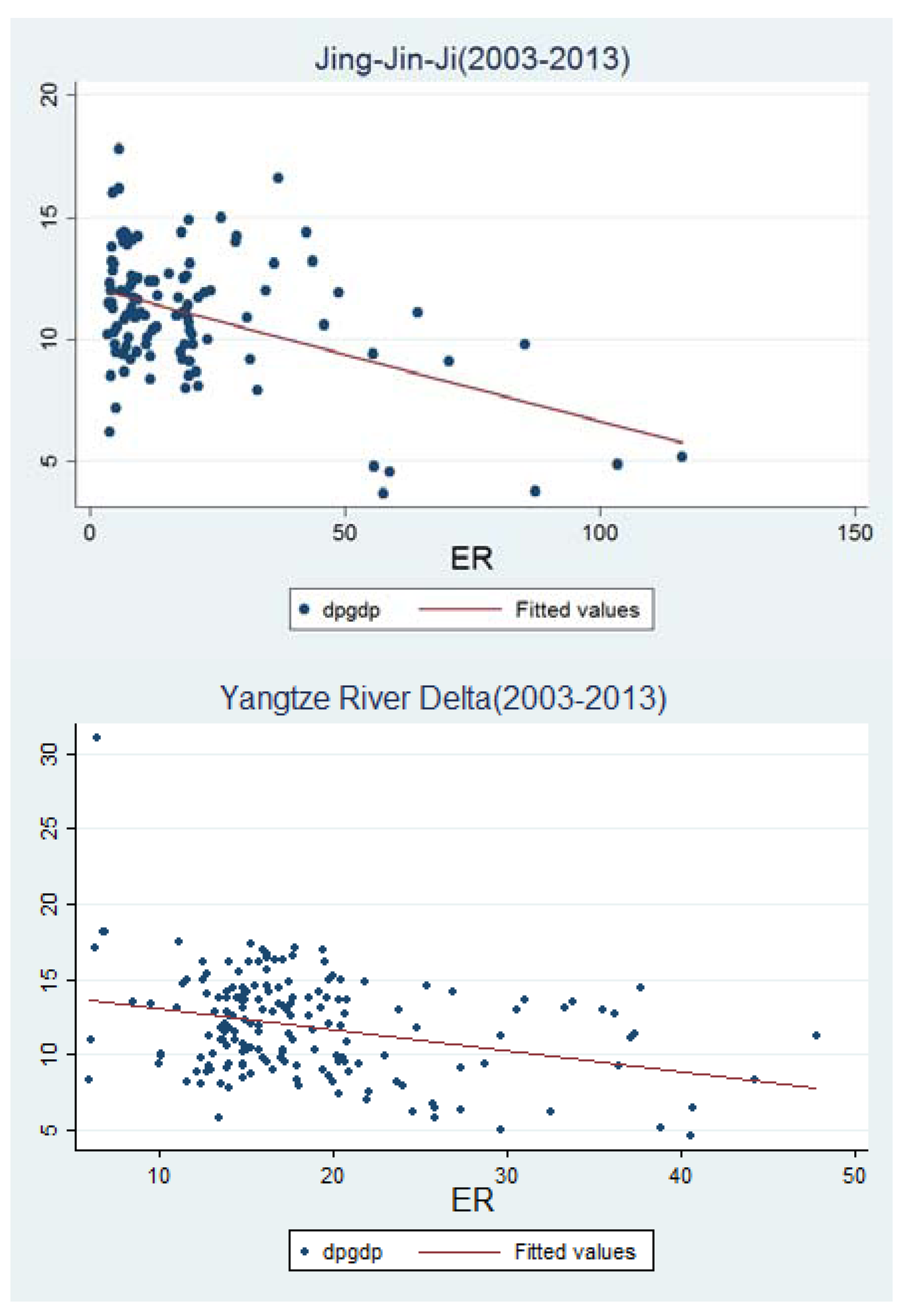
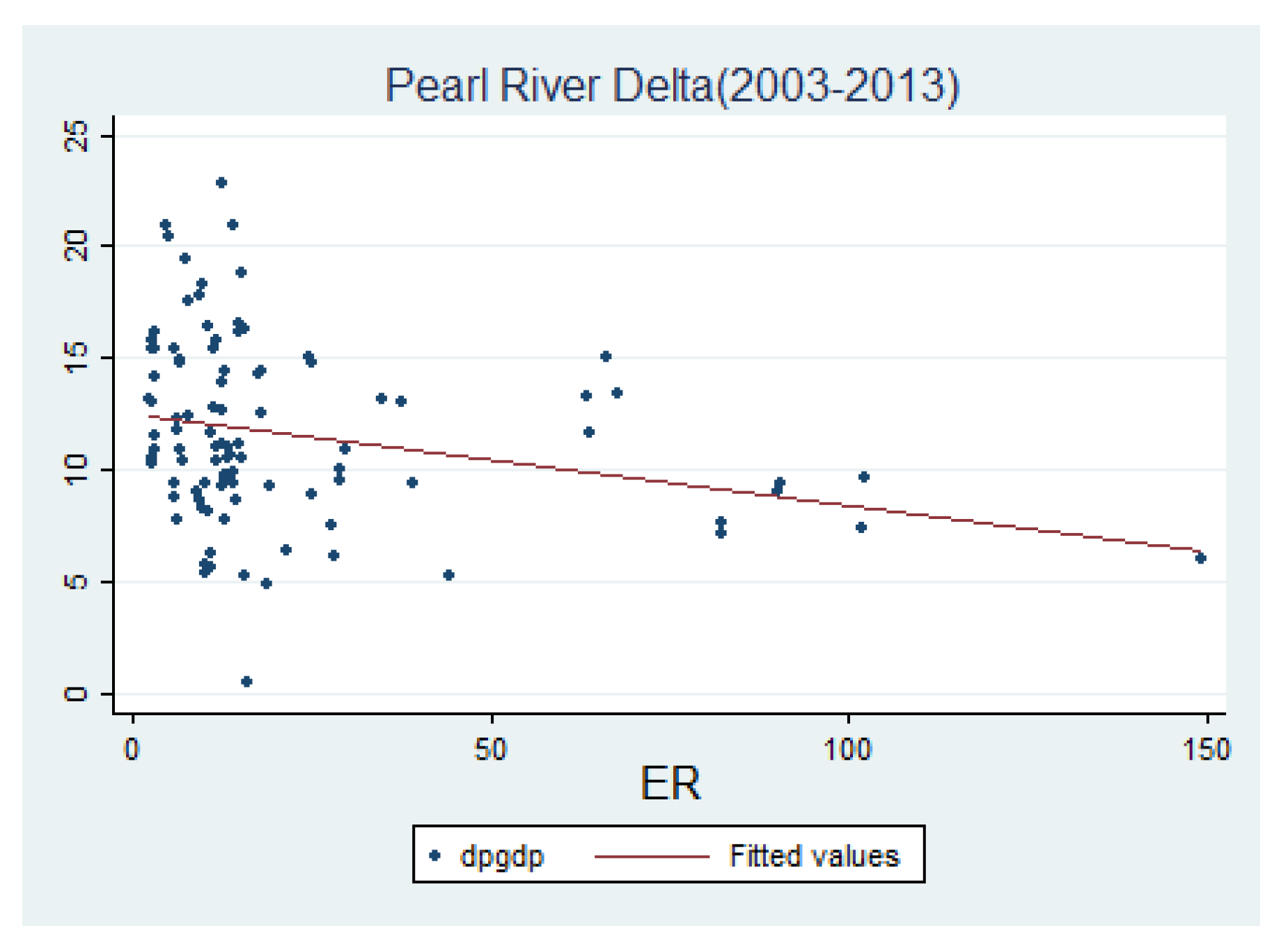
We observe that the results are consistent with theory and our predictions. Concerning our core variable, environmental regulation, it seems to be an important factor for urban economic growth. In all of the three estimate results, the estimated coefficients of lnERt−1 are always negative and consistently significant at the 1% level, indicating that more stringent environmental regulations deter urban economic growth. Comparing the three estimate results, we find that there are significant differences in the extent of impact of environmental regulation on economic growth. Among them, the coefficient of lnERt−1 in JJJ is the smallest, which is −0.054. It shows that, for cities in JJJ, the stringency of the environmental regulation increased by 1%, and the growth rate of GDP per capita decreased by 0.054%. For YRP, the coefficient of lnERt−1 is −0.147, which sits in the middle of the three. It indicates that the environmental regulation stringency increased by 1%, and the growth rate of GDP per capita decreased by 0.147%. In PRD, the elasticity value is −0.494, which means that the environmental regulation stringency increased by 1%, and the per capita GDP growth rate decreased by 0.494%. Environmental regulation has the greatest impact on cities of PRD, which may be due to the industrial structure of PRD. In PRD, most peripheral cities’ industries mainly rely on OEM, which produce some pollution and are sensitive to the pollution cost. Therefore, the impact of environmental regulation in PRD is larger than for the other two urban agglomerations.

5.2.2. The Long-Term Effects of Environmental Regulation on Economic Growth

In order to determine the long-term effects of environmental regulation on economic growth, we have introduced the square of environmental regulation variables in regression equations to determine whether the change in environmental regulation levels has a threshold effect on economic growth in the three urban agglomerations. From the results of Column (2) in Table 2, Table 3 and Table 4, it can be found that lnERt−1 and its square are not significant at the 10% level for the three regression results. Even if the confidence level is expanded to 20%, the coefficients are still not significant for the three regression results, which shows that the environmental regulation has no long-term effect on economic growth.
This result may be due to the following two reasons. Firstly, the long-term effect of environmental regulation on economic growth has not been shown in the period of our study (2003–2013). Even though environmental regulation can promote economic growth through industrial upgrading, the long-term growth effects are not significant during this period. Secondly, though the threshold effect exists, the threshold value of the environmental regulation index may be too low or too high. For JJJ and YRD, ER and economic growth show an inverted U shaped relationship which means that the impact of environmental regulation on economic growth increases after a period of suppression. However, ER index’s threshold values are 7.389 and 8.331, respectively, which are less than most ER indexes in our research. For PRD, environmental regulation and economic growth show a U shaped relationship, while the threshold value is 219695, apparently too large and meaningless for this problem.

5.2.3. Channels for the Spillover in the Urban Agglomeration

Column (3)–(6) in Table 2, Table 3 and Table 4 show the regression results of spatial econometric models under the above four weight matrices, respectively. LR, AIC and SC test values show that the SAR model that we used is appropriate. Introducing spatial interaction in spatial econometric models has been advocated by previous researches [66,67]. As Harris et al. [67] observed, “the standard approach using W is that spillovers are entered through the interaction between regions of the dependent or other variables in the model, weighted by W , as the proxies for spatial spillovers.” Therefore, the different spatial weight matrices reflect different types of interaction among cities in the urban agglomeration. In other words, the regression results under different weight matrices shed a light on the significance of spillover effects in different channels, which is very important in exploring the characteristics of the economic network in the urban agglomeration and in analyzing the mechanism of economic interaction among cities in the urban agglomeration.
Analyzing the estimation results of JJJ, YRP and PRD, under four different weight matrices, the estimated coefficient of lnERt−1 is negative and consistently significant. This verifies that our benchmark model is robust, and the impact of environmental regulation on economic growth is consistent with reality. The value of Rho, the coefficient of spatial lag variable W Y , can reflect the spillover effect and spillover channels by its significance.
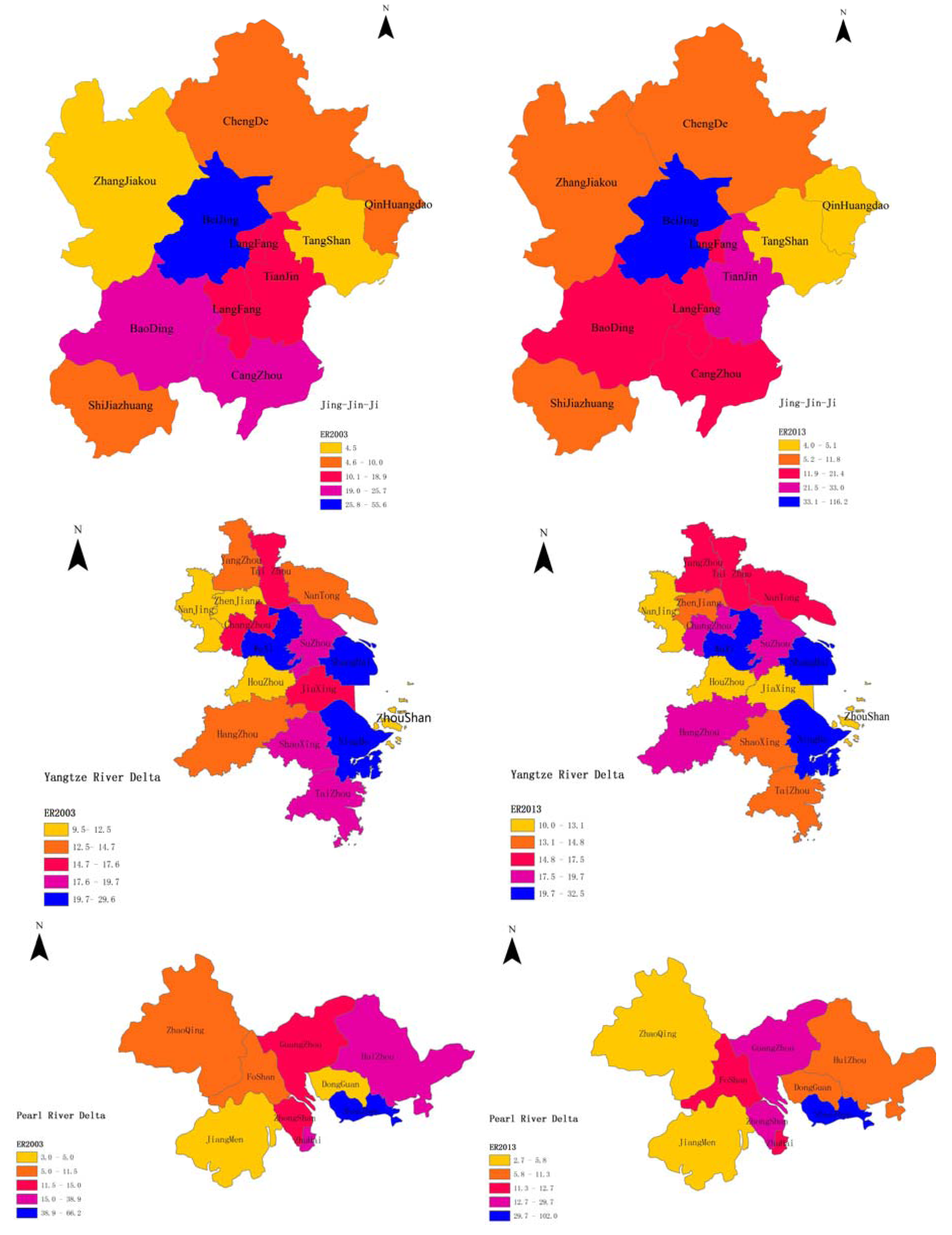
Comparing the estimation results of Rho, we can find that there are differences in the economic spillover channels for the three urban agglomerations. Specifically, for the results of JJJ, Rho value is significant under the weight matrices W 2 and W 3 , but the Rho value under W 2 is only –4.6 × 10⁻⁴, which lacks economic significance. Therefore, the weight matrix W 3 reflects the channels and mechanisms for the economic spillover within JJJ, and the impact is significantly positive. That is, the greater the economic disparity among cities in JJJ is, the stronger the economic spillover effect that occurs. There is a close connection and interaction between cities with a huge economic gap between them, which is consistent with the industrial transfer policy of JJJ. Beijing, for example, has been transferring capital steel and other heavy industrial enterprises to Tangshan, Baoding and other surrounding cities since 2005. Since then, the central government further put forward the policy of “transfer the non-capital function” to relieve Beijing’s urban congestion and huge environmental pressure. As such, a series of industrial firms will gradually relocate to Shijiazhuang, Qinhuangdao where the level of economic development is relatively low. It is worth noting that the regression results under W 1 and W 4 are not significant, which shows that the geographical factor and environmental regulation disparity are not important factors affecting the economic spillover of JJJ. This shows that the industrial transfer in JJJ is mostly policy-oriented rather than market-oriented, which is mainly because the enterprises of JJJ are mainly composed of state-owned enterprises, whose business decisions are made by the government and not the market.
As shown in Table 3, for YRP, Rho value is significant under the weight matrices W 1 , W 3 and W 4 , which means that spillover occurs onto neighbors and cities with different economic development levels or with different environmental regulation policies. The Rho value under W 1 is significantly positive, which suggests that neighboring cities in YRP have close interaction with each other, and also have a similar economic growth level, showing signs of collaborative development. The Rho value under W 4 is significantly negative at −0.454. This shows that “zero-sum game” caused by the environmental regulation disparity existing in YRD. The firms transfer from cities with more stringent environmental regulation policies to cities with laxer policies, so the growth rates in these two kinds of cities show a negative correlation. Obviously, when environmental regulation disparity exists, some cities’ rapid economic growth occurs at the expense of the cities with more stringent environmental regulations. Similarly, the Rho value under W 3 shows that the cities with economic disparity also experience the “zero-sum game”.
For PRD, the estimation results show that the Rho value is significant under matrices W 2 and W 4 . The Rho value under W 2 is only 0.001, which is meaningless for economic interpretation. What is interesting is that the Rho value under W 4 is significantly positive, and the value is 0.431, which is significantly different from the results of JJJ and YRD, indicating that the cities with environmental regulation disparity have a positive correlation with each other. To explore the reason for this, we can draw some insights from the “vacating cage to change bird” policy advocated by the Guangdong provincial government. The cities with environmental regulation disparity may be presented with opportunities to grow from the industrial transfer. For cities with more rigorous environmental regulations, they clear the polluting firms away and then give room for more suitable enterprises to move in. Through this process, these cities achieve the goal of updating their development patterns to ones that are more sustainable. For cities with more lenient environmental regulations, firms move in and bring demand for employment, which gives peripheral cities a chance to achieve a faster economic growth rate. It can be seen that environmental regulation disparity in PRD has an important role in promoting the overall level of sustainable growth, and the “Race to the bottom” phenomenon has not been evident.
Comparing the spatial econometric regression results of the three urban agglomerations, there are great differences in the spillover effects and spillover channels. Specifically, environmental regulation disparity has become an important spillover channel for YRD and PRD. In these two urban agglomerations, environmental regulation in PRD has promoted the coordinated growth through industrial transfer and industrial structure upgrades. For YRD, there is a trade-off between cities with environmental regulation disparities, and the whole economy falls into the “zero-sum game” dilemma. The reason for this situation is mostly due to the benefits of industrial structure upgrading in cities with severe environmental regulations that cannot compensate for the losses arising from industrial transfer. In JJJ, the impact of environmental regulation disparity on the spillover effect is not significant, and political factors play an important role in the spillover process. In summary, environmental regulation significantly affects cities’ economic growth, but only in YRD and PRD does environmental regulation disparity become a spillover channel through the process of industrial transfer.

6. Conclusions

This paper examined the influence of environmental regulation on the sustainable economic growth of urban agglomerations. Using the NEG model as the theoretical framework, we illustrated how environmental regulation influenced firms’ location choices and urban economic growth. By developing a complex index expressing the stringency of environmental regulation for China’s three largest urban agglomerations (Jing-Jin-Ji, the Yangtze River Delta and the Pearl River Delta), this research revealed the negative effect of environmental regulation on urban economic growth and different spillover mechanisms across urban agglomerations.
Empirical results of the benchmark model showed that environmental regulation had a consistently significant negative effect on economic growth in the three urban agglomerations, verifying the propositions proposed in the model. Cities with more lenient environmental regulations had a higher growth rate. Furthermore, we tested whether environmental regulation had a long-term effect on economic growth, and found no sufficient evidence regarding the existence of long-term effects in all three urban agglomerations.
In an attempt to identify the channels through which economic spillover occurs in the urban agglomeration, we used different weight matrices to illustrate the different economic networks of the urban agglomeration, and demonstrated that the spillover mechanisms in different urban agglomerations varied. Specifically, environmental regulation disparity was a spillover channel for the Yangtze River Delta and the Pearl River Delta, while the spillover effect of this channel was not significant for Jing-Jin-Ji. Besides, environmental regulation disparity in the Pearl River Delta promoted regional development, while it triggered fiercer competition among cities in the Yangtze River Delta.

Acknowledgments

This work has been supported by National Social Science Foundation of China (No. 11&ZD159), National Natural Science Foundation of China (41430637; 41329001), and National Science Foundation of USA (1416509).

Author Contributions

Zhaohui Chong and Chenglin Qin co-designed and performed research. Xinyue Ye provided the method of data analysis and modified the draft. All authors read and approved the final manuscript.

Conflicts of Interest

The authors declare no conflict of interest.

Appendix A. List of cities

Table A1. List of cities and most important information.
CityUrban AgglomerationER IndexGrowth Rate
Bei JingJing-Jin-Ji73.097.12
Tian JinJing-Jin-Ji22.9811.66
Shi Jia zhuangJing-Jin-Ji10.3511.12
Tang ShanJing-Jin-Ji6.0911.96
Qin Huang daoJing-Jin-Ji8.1710.48
Bao DingJing-Jin-Ji18.6711.01
Zhang Jia kouJing-Jin-Ji5.1011.32
Cheng DeJing-Jin-Ji6.1312.58
Cang ZhouJing-Jin-Ji32.0012.57
Lang FangJing-Jin-Ji18.7910.72
Shang HaiYangtze River Delta34.468.38
Nan JingYangtze River Delta13.5211.07
Wu XiYangtze River Delta20.2511.46
Chang ZhouYangtze River Delta15.7511.68
Su ZhouYangtze River Delta19.3510.12
Nan TongYangtze River Delta15.4314.12
Yang ZhouYangtze River Delta17.0713.87
Zhen JiangYangtze River Delta15.1212.90
Tai ZhouYangtze River Delta15.1114.09
Hang ZhouYangtze River Delta16.3410.79
Ning BoYangtze River Delta24.3310.55
Jia XingYangtze River Delta14.4511.54
Hu ZhouYangtze River Delta12.7312.42
Shao XingYangtze River Delta18.4811.33
Zhou ShanYangtze River Delta9.0315.01
Taii ZhouYangtze River Delta33.3410.63
Guang ZhouPearl River Delta24.9110.64
Shen ZhenPearl River Delta87.229.94
Zhu HaiPearl River Delta12.8310.74
Fo ShanPearl River Delta11.6412.44
Jiang MenPearl River Delta5.6811.38
Zhao QingPearl River Delta3.9513.39
Hui ZhouPearl River Delta23.3911.96
Dong GuanPearl River Delta8.6911.69
Zhong ShanPearl River Delta13.4612.54

Appendix B. Data Summary

Table B1. Descriptive statistics for variables used in estimations.
Dataset of Jing-Jin-Ji
VariableObsMeanStd. Dev.MinMax
lndpgdp1102.3690320.27977511.3083332.879198
lner1102.6116960.8542081.2803184.755158
lnpop1106.5262940.57221135.610577.656715
lnexpen1108.0410190.89600056.31545910.25969
lnk1109.5544220.78422077.66544111.13821
Dataset of the Yangtze River Delta
VariableObsMeanStd. Dev.MinMax
lndpgdp1762.4335690.29205431.5260563.437208
lner1762.8421030.37443991.7866783.867998
lnpop1766.1534970.62694674.5726477.789516
lnexpen1767.255581.8012881.1580259.74724
lnk17610.030260.61785138.30182711.30529
Dataset of the Pearl River Delta
VariableObsMeanStd. Dev.MinMax
lndpgdp992.3716050.473177−0.6931473.127383
lner992.5823490.93502770.76264655.006705
lnpop996.182550.61501324.9041637.764538
lnexpen998.2471630.70551526.7947349.674568
lnk999.5994270.55905468.07489311.00911

References

  1. World Bank. China Water Quality Management: Policy and Institutional Considerations; World Bank: Washington, DC, USA, 2006. [Google Scholar]
  2. World Bank. Cost of Pollution in China: Economic Estimates of Physical Damages; World Bank: Washington, DC, USA, 2007. [Google Scholar]
  3. China Daily. Promise of Iron Fist against Pollution. Available online: http://www.chinadaily.com.cn/china/2013npc/2013–03/18/content_16314997.htm (accessed on 6 November 2015).
  4. Kostka, G.; Moslener, U.; Andreas, J. Barriers to increasing energy efficiency: Evidence from small-and medium-sized enterprises in China. J. Clean. Prod. 2013, 57, 59–68. [Google Scholar]
  5. Porter, M.E.; van der Linde, C. Green and competitive: Ending the stalemate. Harv. Bus. Rev. 1995, 73, 120–134. [Google Scholar]
  6. Pearce, F. Confessions of an Eco-Sinner: Tracking down the Sources of My Stuff; Beacon Press: Boston, MA, USA, 2008. [Google Scholar]
  7. Jorgenson, D.W.; Wilcoxen, P.J. Environmental regulation and US economic growth. Rand J. Econ. 1990, 21, 314–340. [Google Scholar] [CrossRef]
  8. Kostka, G. Barriers to the Implementation of Environmental Policies at the Local Level in China. Available online: http://ssrn.com/abstract=2487614 (accessed on 1 August 2015).
  9. Sigman, H. Transboundary spillovers and decentralization of environmental policies. J. Environ. Econ. Manag. 2005, 50, 82–101. [Google Scholar] [CrossRef]
  10. Bernauer, T.; Kuhn, P.M. Is there an environmental version of the Kantian peace? Insights from water pollution in Europe. Eur. J. Int. Relat. 2010, 16, 77–102. [Google Scholar]
  11. Cai, H.; Chen, Y.; Gong, Q. Polluting thy neighbor: Unintended consequences of China’s pollution reduction mandates. J. Environ. Econ. Manag. 2015. [CrossRef]
  12. Batten, D.F. Network cities: Creative urban agglomerations for the 21st century. Urban Stud. 1995, 32, 313–327. [Google Scholar] [CrossRef]
  13. De Goei, B.; Burger, M.J.; van Oort, F.G.; Kitson, M. Functional polycentrism and urban network development in the Greater South East, United Kingdom: Evidence from commuting patterns, 1981–2001. Reg. Stud. 2010, 44, 1149–1170. [Google Scholar] [CrossRef]
  14. Zheng, X.P. Economies of network, urban agglomeration, and regional development: A theoretical model and empirical evidence. Reg. Stud. 2007, 41, 559–569. [Google Scholar] [CrossRef]
  15. Huggins, R.; Thompson, P. A Network-based view of regional growth. J. Econ. Geogr. 2014, 14, 511–545. [Google Scholar] [CrossRef]
  16. Gray, W.B.; Shadbegian, R.J. The Environmental Performance of Polluting Plants: A Spatial Analysis. J. Reg. Sci. 2007, 47, 63–84. [Google Scholar] [CrossRef]
  17. Liang, X.; Zhang, W.; Chen, L.; Deng, F. Sustainable Urban Development Capacity Measure—A Case Study in Jiangsu Province, China. Sustainability 2016, 8, 270. [Google Scholar] [CrossRef]
  18. Ashford, N.A.; Hall, R.P. The importance of regulation-induced innovation for sustainable development. Sustainability 2011, 3, 270–292. [Google Scholar] [CrossRef]
  19. Popp, D. ENTICE: Endogenous Technological Change in the DICE model of global warming. J. Environ. Econ. Manag. 2004, 48, 742–768. [Google Scholar] [CrossRef]
  20. Dernbach, J.C.; Mintz, J.A. Environmental laws and sustainability: An introduction. Sustainability 2011, 3, 531–540. [Google Scholar] [CrossRef]
  21. Abdullah, S.; Morley, B. Environmental taxes and economic growth: Evidence from panel causality tests. Energ. Econ. 2014, 42, 27–33. [Google Scholar] [CrossRef] [Green Version]
  22. McGowan, F. Regulating innovation: European responses to shale gas development. Environ. Polit. 2014, 23, 41–58. [Google Scholar] [CrossRef]
  23. Yin, J.; Zheng, M.; Chen, J. The effects of environmental regulation and technical progress on CO2 Kuznets curve: An evidence from China. Energy Policy 2015, 77, 97–108. [Google Scholar] [CrossRef]
  24. Jaffe, A.B.; Palmer, K. Environmental regulation and innovation: A panel data study. Rev. Econ. Stat. 1997, 79, 610–619. [Google Scholar] [CrossRef]
  25. Brunnermeier, S.B.; Cohen, M.A. Determinants of environmental innovation in US manufacturing industries. J. Environ. Econ. Manag. 2003, 45, 278–293. [Google Scholar] [CrossRef]
  26. Johnstone, N.; Labonne, J.; Thevenot, C. Environmental policy and economies of scope in facility-level environmental practices. Environ. Econ. Policy Stud. 2008, 9, 145–166. [Google Scholar] [CrossRef]
  27. Johnstone, N. Environmental Policy and Corporate Behaviour; Edward Elgar Publishing: Cheltenham, UK, 2007. [Google Scholar]
  28. Lanoie, P.; Laurent-Lucchetti, J.; Johnstone, N.; Stefan, A. Environmental policy, innovation and performance: New insights on the Porter hypothesis. J. Econ. Manag. Strat. 2011, 20, 803–842. [Google Scholar] [CrossRef]
  29. Keller, W.; Levinson, A. Pollution abatement costs and foreign direct investment inflows to US states. Rev. Econ. Stat. 2002, 84, 691–703. [Google Scholar] [CrossRef]
  30. Raspiller, S.; Riedinger, N. Do Environmental Regulations Influence the Location Behavior of French Firms? Land Econ. 2008, 84, 382–395. [Google Scholar] [CrossRef]
  31. Kheder, S.B.; Zugravu, N. Environmental regulation and French firms location abroad: An economic geography model in an international comparative study. Ecol. Econ. 2012, 77, 48–61. [Google Scholar] [CrossRef]
  32. Goodman, J.B.; Pauly, L.W. The obsolescence of capital controls?: Economic management in an age of global markets. World Polit. 1993, 46, 50–82. [Google Scholar]
  33. Holzinger, K.; Knill, C. Competition and cooperation in environmental policy: Individual and interaction effects. J. Public Policy 2004, 24, 25–47. [Google Scholar] [CrossRef]
  34. Drezner, D.W. Globalization and policy convergence. Int. Stud. Rev. 2001, 3, 53–78. [Google Scholar] [CrossRef]
  35. Ioppolo, G.; Cucurachi, S.; Salomone, R.; Saija, G.; Shi, L. Sustainable Local Development and Environmental Governance: A Strategic Planning Experience. Sustainability 2016, 8, 180. [Google Scholar] [CrossRef]
  36. Becker, R.; Henderson, V. Effects of air quality regulations on polluting industries. J. Polit. Econ. 2000, 108, 379–421. [Google Scholar] [CrossRef]
  37. Kahn, M.E.; Mansur, E.T. Do local energy prices and regulation affect the geographic concentration of employment? J. Public Econ. 2013, 101, 105–114. [Google Scholar] [CrossRef]
  38. Bovenberg, A.L.; de Mooij, R.A. Environmental levies and distortionary taxation. Am. Econ. Rev. 1994, 84, 1085–1089. [Google Scholar]
  39. Ricci, F. Channels of transmission of environmental policy to economic growth: A survey of the theory. Ecol. Econ. 2007, 60, 688–699. [Google Scholar] [CrossRef]
  40. Aloi, M.; Tournemaine, F. Inequality, growth, and environmental quality trade-offs in a model with human capital accumulation. Can. J. Econ. 2013, 46, 1123–1155. [Google Scholar] [CrossRef]
  41. Smulders, S.; Toman, M.; Withagen, C. Growth theory and ‘green growth’. Oxf. Rev. Econ. Policy 2014, 30, 423–446. [Google Scholar] [CrossRef]
  42. Håkansson, H. Technological collaboration in industrial networks. Eur. Manag. J. 1990, 8, 371–379. [Google Scholar] [CrossRef]
  43. Snyder, D.; Kick, E.L. Structural position in the world system and economic growth, 1955–1970: A multiple-network analysis of transnational interactions. Am. J. Sociol. 1979, 84, 1096–1126. [Google Scholar] [CrossRef]
  44. Oerlemans, L.A.G.; Meeus, M.T.H.; Boekema, F.W.M. Do networks matter for innovation? The usefulness of the economic network approach in analysing innovation. Tijdschr. Econ. Soc. Geogr. 1998, 89, 298–309. [Google Scholar] [CrossRef]
  45. Chantarat, S.; Barrett, C.B. Social network capital, economic mobility and poverty traps. J. Econ. Inequal. 2012, 10, 299–342. [Google Scholar] [CrossRef]
  46. Fan, Y.; Ren, S.; Cai, H. The state’s role and position in international trade: A complex network perspective. Econ. Model 2014, 39, 71–81. [Google Scholar] [CrossRef]
  47. Kim, D.R. Do local policy networks deter the race to the bottom in environmental regulation? The case of South Korea. Environ. Plan. C 2011, 29, 1037–1053. [Google Scholar] [CrossRef]
  48. Acemoglu, D.; García-Jimeno, C.; Robinson, J.A. State Capacity and Economic Development: A Network Approach. Am. Econ. Rev. 2015, 105, 2364–2409. [Google Scholar] [CrossRef]
  49. Topa, G.; Zenou, Y. Neighborhood versus Network Effects. In Handbook of Regional and Urban Economics; Duranton, G., Henderson, V., Strange, W., Eds.; Elsevier Publisher: Amsterdam, The Netherlands, 2015; Volume 5. [Google Scholar]
  50. Bai, C.E.; Ma, H.; Pan, W. Spatial spillover and regional economic growth in China. China Econ. Rev. 2012, 23, 982–990. [Google Scholar] [CrossRef]
  51. Corrado, L.; Fingleton, B. Where is the economics in spatial econometrics? J. Reg. Sci. 2012, 52, 210–239. [Google Scholar] [CrossRef]
  52. Head, K.; Mayer, T. Market potential and the location of Japanese investment in the European Union. Rev. Econ. Stat. 2004, 86, 959–972. [Google Scholar] [CrossRef]
  53. Checherita-Westphal, C.; Rother, P. The impact of high government debt on economic growth and its channels: An empirical investigation for the euro area. Eur. Econ. Rev. 2012, 56, 1392–1405. [Google Scholar] [CrossRef]
  54. Elhorst, J.P. Applied spatial econometrics: Raising the bar. Spat. Econ. Anal. 2010, 5, 9–28. [Google Scholar] [CrossRef]
  55. Anselin, L. Spatial Econometrics: Methods and Models; Springer Science & Business Media: Heidelberg, Germany, 2013. [Google Scholar]
  56. Bavaud, F. Spatial Weights: Constructing Weight-Compatible Exchange Matrices from Proximity Matrices; Springer International Publishing: Berlin, Germany, 2014. [Google Scholar]
  57. Greenhut, M.L.; Norman, G.; Hung, C.S. The Economics of Imperfect Competition: A Spatial Approach; Cambridge University Press: London, UK, 1987. [Google Scholar]
  58. Fingleton, B.; Le Gallo, J. Estimating spatial models with endogenous variables, a spatial lag and spatially dependent disturbances: Finite sample properties. Pap. Reg. Sci. 2008, 87, 319–339. [Google Scholar] [CrossRef]
  59. Sanchez-Vargas, A.; Mansilla-Sanchez, R.; Aguilar-Ibarra, A. An empirical analysis of the nonlinear relationship between environmental regulation and manufacturing productivity. J. Appl.Econ. 2013, 16, 357–372. [Google Scholar] [CrossRef]
  60. Levinson, A. Environmental regulatory competition: A status report and some new evidence. Natl. Tax J. 2003, 56, 91–106. [Google Scholar] [CrossRef]
  61. National Bureau of Statistics of China (NBSC). China City Statistical Yearbook, 2004–2014; China Statistics Press: Beijing, China, 2004–2014. (In Chinese)
  62. HeBei Statistical Bureau. HeBei Economic Yearbook, 2004–2014; China Statistics Press: Beijing, China, 2004–2014. (In Chinese)
  63. JiangSu Statistical Bureau. JiangSu Statistical Yearbook, 2004–2014; China Statistics Press: Beijing, China, 2004–2014. (In Chinese)
  64. ZheJiang Statistical Bureau. ZheJiang Statistical Yearbook, 2004–2014; China Statistics Press: Beijing, China, 2004–2014. (In Chinese)
  65. Guangdong Statistical Bureau. GuangDong Statistical Yearbook, 2004–2014; China Statistics Press: Beijing, China, 2004–2014. (In Chinese)
  66. Oud, J.H.L.; Folmer, H.A. Structural equation approach to models with Spatial Dependence. Geogr. Anal. 2008, 40, 152–166. [Google Scholar] [CrossRef]
  67. Harris, R.; Moffat, J.; Kravtsova, V. In Search of ‘W’. Spat. Econ. Anal. 2011, 6, 249–270. [Google Scholar] [CrossRef]
Figure 1. Study areas in China: JJJ (north), YRD (east) and PRD (south).
Sustainability 08 00467 g001
Figure 2. The dynamic change of the ER Index in the three urban agglomerations.
Sustainability 08 00467 g002
Figure 3. Relationship between ER index and GDP per capita.
Sustainability 08 00467 g003aSustainability 08 00467 g003b
Table 1. ER Index of Jing-Jin-Ji, the Yangtze River Delta and the Pearl River Delta.
YearJJJYRDPRD
AverageMaxC.VAverageMaxC.VAverageMaxC.V
200317.655.60.8718.137.70.4119.666.31.04
200621.485.41.1818.437.30.4117.867.51.10
200920.158.90.9119.744.20.5131.7149.41.44
201324.4116.21.3717.332.50.3222.3102.11.38
Table 2. Model estimate results (Jing-Jin-Ji).
(1)(2)(3)(4)(5)(6)
lnERt−1−0.054 *0.164−0.055 **−0.052 **−0.053 **−0.043
(−1.94)(1.07)(−2.04)(−2.11)(−2.01)(−1.50)
lnPop−0.044−0.037−0.0424−0.073 *−0.057−0.039
(−1.06)(−0.91)(−1.06)(−1.93)(−1.43)(−0.98)
lnExpen−0.253 ***−0.200 ***−0.254 ***−0.289 ***−0.262 ***−0.242 ***
(−6.34)(−3.69)(−6.56)(−7.86)(−6.82)(−6.08)
lnk0.209 ***0.160 **0.210 ***0.233 ***0.219 ***0.194 ***
(4.10)(2.63)(4.25)(5.06)(4.48)(3.81)
recession−0.268 ***−0.267 ***−0.249 ***−0.277 ***−0.178 **−0.350 ***
(−5.11)(−5.12)(−4.07)(−5.87)(−2.49)(−3.87)
lnERt−12 −0.041
(−1.44)
cons2.981 ***2.717 ***2.825 ***3.429 ***2.418 ***3.423 ***
(8.96)(7.19)(6.54)(10.85)(5.36)(6.64)
Rho 0.059−4.6e-04 ***0.247 *−0.182
(0.54)(−4.33)(1.75)(−1.10)
Prob > Chi2(1) 0.58730.00000.07970.2724
Likelihood Ratio Test 0.294618.72043.07171.2044
Log AIC −3.8168−3.8439−3.8314−3.8083
Log SC −3.6695−3.6966−3.6841−3.6610
R20.61630.62390.74570.75250.74940.7435
N. of obs.111111111111111111
Notes: A full set of city specific and period specific effects are also included for Columns (1)–(6). Standard errors clustered at county-year level are reported in parentheses. *** p < 0.01. ** p < 0.05. * p < 0.1.
Table 3. Model estimate results (the Yangtze River Delta).
(1)(2)(3)(4)(5)(6)
lnERt−1−0.147 ***0.394−0.127 ***−0.143 ***−0.137 ***−0.087 *
(−2.77)(1.07)(−2.68)(−2.71)(−2.70)(−1.62)
lnPop−0.115 ***−0.124 ***−0.129 ***−0.121 ***−0.104 ***−0.121 ***
(−3.66)(−3.88)(−4.58)(−3.32)(−3.43)(−4.04)
lnExpen−0.012−0.010−0.012−0.012−0.010−0.012
(−1.53)(−1.22)(−1.62)(−1.59)(−1.27)(−1.58)
lnk−0.088 ***−0.099 ***−0.091 ***−0.091 ***−0.081 **−0.111 ***
(−2.68)(−2.96)(−3.11)(−2.68)(−2.55)(−3.48)
recession−0.294 ***−0.283 ***−0.135 ***−0.292 ***−0.451 ***−0.488 ***
(−7.32)(−6.94)(−2.94)(−7.38)(−6.13)(−6.77)
lnERt−12 −0.093
(−1.48)
cons4.693 ***4.067 ***3.643 ***4.771 ***5.559 ***5.966 ***
(12.88)(7.29)(9.65)(10.87)(11.30)(11.25)
Rho 0.419 ***−7.11e–06−0.397 **−0.454 ***
(5.48)(−0.31)(−2.50)(−3.17)
Prob > Chi2(1) 0.00000.75740.01230.0015
Likelihood Ratio Test 30.01940.09546.273310.0359
Log AIC −3.4808−3.5256−3.5303−3.4986
Log SC −3.3727−3.4175−3.4222−3.3905
R20.58220.58760.66090.67580.67730.6670
N. of obs.176176176176176176
Notes: A full set of city specific and period specific effects are also included for Columns (1)–(6). Standard errors clustered at county-year level are reported in parentheses. *** p < 0.01. ** p < 0.05. * p < 0.1.
Table 4. Model estimate results (the Pearl River Delta).
(1)(2)(3)(4)(5)(6)
lnERt−1−0.494 ***−0.413−0.478 ***−0.470 ***−0.493 ***−0.469 ***
(−4.21)(−1.23)(−4.01)(−4.22)(−4.19)(−4.02)
lnPop0.3530.3610.3210.2780.3490.277
(0.80)(0.81)(0.72)(0.66)(0.78)(0.63)
lnExpen0.01900.016−0.011−0.0800.016−0.072
(0.07)(0.05)(−0.04)(−0.30)(0.05)(−0.25)
lnk0.1040.1020.1230.1680.1060.151
(0.39)(0.38)(0.45)(0.65)(0.39)(0.56)
recession−0.675 ***−0.670 ***−0.591 ***−0.455 ***−0.668 ***−0.408 *
(−4.62)(−4.52)(−3.13)(−2.93)(−3.18)(−1.93)
lnERt−12 −0.0167
(−0.25)
cons0.6740.5840.5900.5330.6710.241 ***
(0.23)(0.20)(0.20)(0.19)(0.23)(0.08)
Rho 0.1100.001 ***0.0110.431 *
(0.70)(3.15)(0.05)(1.73)
Prob > Chi2(1) 0.48770.00230.96350.0870
Likelihood Ratio Test 0.48609.90400.00212.9983
Log AIC −2.0771−2.1828−2.0714−2.1064
Log SC −1.8150−1.9207−1.8093−1.8443
R20.49840.49880.53810.58440.53550.5515
N. of obs.999999999999
Notes: A full set of city specific and period specific effects are also included for Columns (1)–(6). Standard errors clustered at county-year level are reported in parentheses. *** p < 0.01. ** p < 0.05. * p < 0.1.

