Evaluation of Thermal Anomalies in Multi-Boreholes Field Considering the Effects of Groundwater Flow

Abstract

In this paper, the performance of multiple boreholes (multi-BHEs) field is evaluated by considering the groundwater flow. Optimization strategies are presented to mitigate thermal anomalies in the BHEs field. This study shows that groundwater flow greatly improves the heat transfer but causes thermal anomalies downstream. To overcome this problem, a heat transfer model is established for multi-boreholes based on temperature field superposition and moving finite line source model (MFLS). The MFLS multi-boreholes model considers the axial effect and groundwater flow and produces results in agreement with the field tested data of a 4 × 4 boreholes field. Using a dynamic annual load pattern, the long-term performance of the 4 × 4 boreholes field is analyzed. Three dynamic diurnal cooling load models are proposed to evaluate the temperature changes in the underground. The intermittent load model could reduce the local temperature anomalies in downstream tubes. The optimization model for cooling cases for multi-BHEs is elaborated to keep the outlet temperature as low as possible and minimize the extreme temperature anomalies, and by this, ultimately improve the system performance. Furthermore, the temperature variations and thermal anomalies downstream of multi-BHEs are investigated by evaluating the arrangement optimization and load optimization. The results show that the optimization could mitigate thermal anomalies downstream and reduce the rate of temperature imbalance of the BHEs field.

1. Introduction

In China, with the implementation of energy conservation and emissions reduction policies, the vertical ground source heat pump (GSHP) system is widely used because of its high efficiency, environmental friendliness, and low running cost. Borehole heat exchangers (BHEs) that are usually 100–150 m deep with a diameter of 0.10–0.15 m are the most important components of the GSHP system. Subsurface thermal properties around BHEs and groundwater flow greatly influence the temperature distribution around the BHEs.

In order to estimate the heat transfer, many analytical or numerical models for designing and analyzing have been developed: the infinite line source model (ILS) [1] and cylindrical heat source model [2] were widely used for the thermal analysis of BHEs because of their simplicity and high speed in computation. Based on the cylindrical source model, Bernier et al. [3] suggested a multiple load aggregation algorithm to calculate the performance of a single borehole under variable load. Fossa. M et al. [4] developed the cylindrical heat source model by using multiple load aggregation algorithms to simulate hourly energy variations. Eskilson [5] proposed a finite line source (FLS) model for a single borehole with finite length by using the finite-difference method and Zeng et al. [6] improved the FLS model by imposing a constant temperature at the ground surface. Lamarche and Beauchamp [7] developed alternative forms for the FLS model with shorter computation time. Bandos. T.V et al. [8] presented a three-dimensional finite line source (FLS) model for BHEs that considered the prevailing geothermal gradient and allowed arbitrary changes in ground surface temperature. The g-functions calculated by Eskilson [5] are extended to shorter time steps, [9] and [10]. Recently, it has been improved by Monzó P [11] using the novel numerical model. Li et al. [12] and Yang et al. [13] proposed and developed an analytical composite-medium line source model, which could accurately evaluate not only the influence of the heat capacity of grouting materials but also the impact of the difference between properties of soil and grout. Recently, Li et al. [14], Hu et al. [15] and Fei Lei et al. [16] developed the composite line source model.

In recent years, with the development of computers and numerical methods, numerical simulation studies are widely used. Finite difference methods [17], finite volume methods [18], and finite element methods [19] have been extensively used for describing the heat transfer mechanisms and thermal response in the subsurface for BHEs. By simplifying the thermal resistance and capacity model, Bauer et al. [20] presented a 3-D numerical model to simulate a thermal response test (TRT) over short and long time scales, and hence, to analyze the fluid temperature variations in the downward and upward tube. With the aid of the MODFLOW, combined use of a spectral method and response model, Pasquier et al. [21] presented a quasi-3D model to simulate the heat transfer of BHEs. Fluid temperature changes for three scenarios were compared to demonstrate the accuracy and validity of the model.

When the permeability is sufficiently high, there may be moving water in the subsurface, and hence, advective transport has to be considered. Some field tests done by Gehlin [22] indicated that groundwater flow influenced the performance of BHEs, even in fracture zones; the smaller groundwater flow rates might cause significantly enhanced heat transfer. Diao et al. [23] presented an analytical solution accounting for the groundwater flow of an infinite line source. Wang et al. [24] implemented an experimental measurement to study the temperature profile of BHEs in subsurface with groundwater flow. Chiasson et al. [25] developed a model to simulate the effects of groundwater flow on BHEs, the results of which showed that the advection of heat by the groundwater flow significantly enhanced the performance of BHEs. Based on the method of G-function, Molina-Giraldo et al. [26] extended the moving infinite line source model to the case of a finite source (Moving Finite Line Source—MFLS). The typical yearly operation of a BHE extracting and injecting heat into in a sandy saturated aquifer is simulated by A. Angelotti, L et.al. [27]. A new analytical model is presented for simulation of ground thermal effects from vertical borehole heat exchangers (BHEs) by Jaime A and Peter Bayer [28]. It accounts for long-term changes in land use and groundwater flow. The results show that land use changes and horizontal advection can overprint anomalies induced by BHEs. Various studies have investigated the heat flow of BHEs by considering the flow of groundwater around the BHEs [29,30,31].

Energy demand is often higher than what a single BHE can provide, and so multi-BHEs are installed and big buildings or district heating systems are supplied by operating multiple BHE fields ([32,33,34]). Field measurements of the temperature distribution of ground around GSHP systems have been reported in the literature [35,36,37,38]. Lazzari [39] studied the long-term performance of double U-tube BHE fields by finite element simulations, but the effects of groundwater movement were negligible. Considering the groundwater flow, Fan et al. [40] evaluated the performance of multi-BHEs connected to a hybrid GSHP system, using a finite volume simulation method. By using a coupled heat conduction–advection model, the performance of various types of BHEs arrays were examined by Jung Chan Choi [41], and optimal BHE arrays were proposed for non-square rectangular arrays.

BHEs are often applied for heating or cooling only, when the heat extraction and injection are not seasonally balanced, ground thermal accumulation will occur and cause a decline of the heat pump’s operational efficiency [29,39]. Rybach and Eugster [42] estimated the duration of thermal recovery as at least as long as the time of operation. There are some auxiliary strategies to alleviate the heat imbalance in the ground [43,44,45]. Recently, a zoning operation strategy, in which only the relatively central part of the GHE runs during the low load season, was adopted by Yu Mingzhi et al. [46] to alleviate the thermal accumulation. Beck et al. [47] recommended several measures, including operation mode adjustment and geometric arrangement, to optimize the performance of the multi-BHEs, but the groundwater flow was not taken into account. Considering the groundwater flow, Jozsef Hecht-Méndez [31] presented a combined simulation optimization procedure for a multiple BHEs field, in which the strategic adjustment of energy extraction rates (loads) of the individual BHEs were considered. A procedure combining analytical simulation and linear optimization for multi-BHEs is presented by Peter Bayer et al. [48]. Peter Bayer has given two ways of tuning BHE fields applied to geothermal heating and cooling: workload optimization of individual BHEs and removal of redundant BHEs for a given arrangement.

Sustainability is in fact an issue that spans the entire lifetime of ground source heat pump (GSHP) systems. Despite the fact that many previous studies have pointed out the positive influence of groundwater flow on BHE performance [27,49], however, it indicates that the groundwater flow caused the thermal anomalies downstream [50]. Thermal interference between the boreholes and the temperature anomalies resulting from the groundwater flow has been inadequately understood. Considering the cooling case only, the groundwater flow would lead to thermal anomalies growing downstream of multi-BHEs. The soil temperature downstream is greatly larger than that of the upstream. This would lead to larger ground temperature differences in the multi-BHEs field and the ground field could not exert its overall heat exchanger efficiency.

When operating a BHE field over years, the interference among the individual boreholes and thermal anomalies downstream will increase the imbalance of the BHEs ground temperature. Different buildings are executed with the different dynamic diurnal load models; how the multi-BHEs temperature field variation and the thermal anomalies changes under different dynamic diurnal load models needs to be studied. On the other hand, several authors [31,47,48] have presented optimizations including arrangement and load assignment for multi-BHEs. They achieved this by minimizing the existing maximal ground temperature differences. However, the heat transfer inside the borehole and thermal short-circuiting between the downward leg of pipe and upward leg of pipe [51] is neglected in these methods.

In the following, firstly, based on the theory of temperature field superposition and dynamic load model, the heat transfer model of MFLS multi-BHEs is established. The model is validated with field data from an experiment and is employed to a BHEs field of 4 × 4 boreholes in order to obtain the temperature rise of typical points in a boreholes field. With the aid of a dynamic annual load pattern, the temperature variation of typical points for ten years using the finite and moving finite line source models were analyzed to reveal the long-term ground temperature considering the groundwater flow. Three dynamic diurnal load models are proposed to analyze how the different diurnal load models influence the performance of multi-BHEs. This could find out the unbalanced characteristics of the multi-BHEs temperature field and the level of thermal anomalies of different buildings. Finally, in order to find the strategies for mitigating thermal anomalies, combined with the quasi 3D model presented by Zeng [6], the optimization model for multi-BHEs is established to keep the outlet fluid temperature as low as possible and minimize the extreme temperature anomalies. The geometric arrangement and workload optimization for individual BHEs are applied to BHEs field of 4 × 4 boreholes in Section 5.

2. Theory

2.1. Finite Line Source Model (FLS)

Based on the finite line source model presented by Eskilson [5], Zeng et al. [6] have given an analytical solution by using a constant temperature for the upper boundary. By using the temporal superposition, L. Lamarche [7] developed the finite line source model in Equation (1):

$$\Delta T{(x,y,z,t)}_{FLS}={\displaystyle \sum _{i=1}^n\frac{q_i-q_{i-1}}{4\pi {\lambda }_s}}{\displaystyle \underset{0}{\overset{H}{\int }}[\frac{erfc(\frac{\sqrt{r^2+{(z-h)}^2}}{2\sqrt{a_{\mathrm{s}}(T_{\mathrm{n}}-T_{i-1})}})}{\sqrt{r^2+{(z-h)}^2}}-\frac{erfc(\frac{\sqrt{r^2+{(z+h)}^2}}{2\sqrt{a_s(T_{\mathrm{n}}-T_{i-1})}})}{\sqrt{r^2+{(z+h)}^2}}]dh}$$

(1)

$$r=\sqrt{x^2+y^2}$$

where △T(x, y, z) is the temperature rise at time t on the position of (x, y, z). r is the distance to theborehole. H is the borehole length. q_i-q_i-1 is the incremental load between two successive hours. λ_s and a_s are the ground thermal conductivity and thermal diffusivity, respectively.

2.2. Moving Finite Line Source Model (MFLS)

Considering the groundwater flow, the temperature response of the moving finite line source (MFLS) model was given by Molina-Giraldo et al. [26]. The principle of temporal superposition was also used to develop the MFLS model, which could be rewritten as Equation (2).

$$\Delta T{(x,y,z)}_{MFLS}={\displaystyle \sum _{i=1}^n\frac{q_i-q_{i-1}}{2\pi {\lambda }_{por}}}\exp (\frac{v_T\mathrm{x}}{2a_{por}})\left\{{\displaystyle \underset{0}{\overset{H}{\int }}(f_1(x,y,z,t_n-t_{i-1})-f_2(x,y,z,t_n-t_{i-1}))dh}\right\}$$

(2)

$$\begin{array}{c}{f}_1(x,y,z,t)=\frac{1}{4r}[\exp (-\frac{v_T\sqrt{r^2+{(z-h)}^2}}{2a_{por}})erfc(\frac{\sqrt{r^2+{(z-h)}^2}-v_T(t_n-t_{i-1})}{2\sqrt{a_{por}(t_n-t_{i-1})}})+\exp (\frac{v_T\sqrt{r^2+{(z-h)}^2}}{2a_{por}})erfc(\frac{\sqrt{r^2+{(z-h)}^2}+v_T(t_n-t_{i-1})}{2\sqrt{a_{por}(t_n-t_{i-1})}})]\\ f_2(x,y,z,t)=\frac{1}{4r}[\exp (-\frac{v_T\sqrt{r^2+{(z+h)}^2}}{2a_{por}})erfc(\frac{\sqrt{r^2+{(z+h)}^2}-v_T(t_n-t_{i-1})}{2\sqrt{a_{por}(t_n-t_{i-1})}})+\exp (\frac{v_T\sqrt{r^2+{(z+h)}^2}}{2a_{por}})erfc(\frac{\sqrt{r^2+{(z+h)}^2}+v_T(t_n-t_{i-1})}{2\sqrt{a_{por}(t_n-t_{i-1})}})]\end{array}$$

(3)

$$\begin{array}{c}{v}_T={\rho }_f{c}_{f}u/{\rho }_{por}{c}_{por}\\ {(\rho c)}_{por}=(1-\varphi ){(\rho c)}_s+\varphi {(\rho c)}_f\\ {\lambda }_{por}=(1-\varphi ){\lambda }_s+\varphi {\lambda }_f\end{array}$$

(4)

2.3. Multi-BHEs Model Considering Groundwater Flow

Based on the MFLS model as in Equation (2), the temperature variation at any arbitrary point in the soil of multi-BHEs fields could be attained by applying the superposition principle to Equation (2) as:

$$\theta {(x,y,z,t)}_{MFLS}={\displaystyle \sum _{j=1}^n\frac{q_j}{2\pi {\lambda }_{por}}\exp (\frac{v_T{\mathrm{X}}_{\mathrm{T}}}{2a_{por}})\left\{{\displaystyle \underset{0}{\overset{H}{\int }}(f_1(x,y,z,t)-f_2(x,y,z,t))dh}\right\}}$$

(5)

$$r_{ij}=\sqrt{{(x-x_i)}^2+{(y-y_j)}^2}$$

$${\mathrm{X}}_{\mathrm{T}}=(x-x_i)$$

where θ(x,y,z,t)_MFLS is the superposition temperature change of arbitrary point (x, y) in depth z caused by every borehole with an energy transfer rate q_j at the time of t. j is the borehole number and n is the total number of the multi-BHEs, q_j is the given energy transfer rate per unit length of the BHE j, X_T is the distance in x-direction to arbitrary point (x, y) with respect to the BHE located at (x_j, y_j).

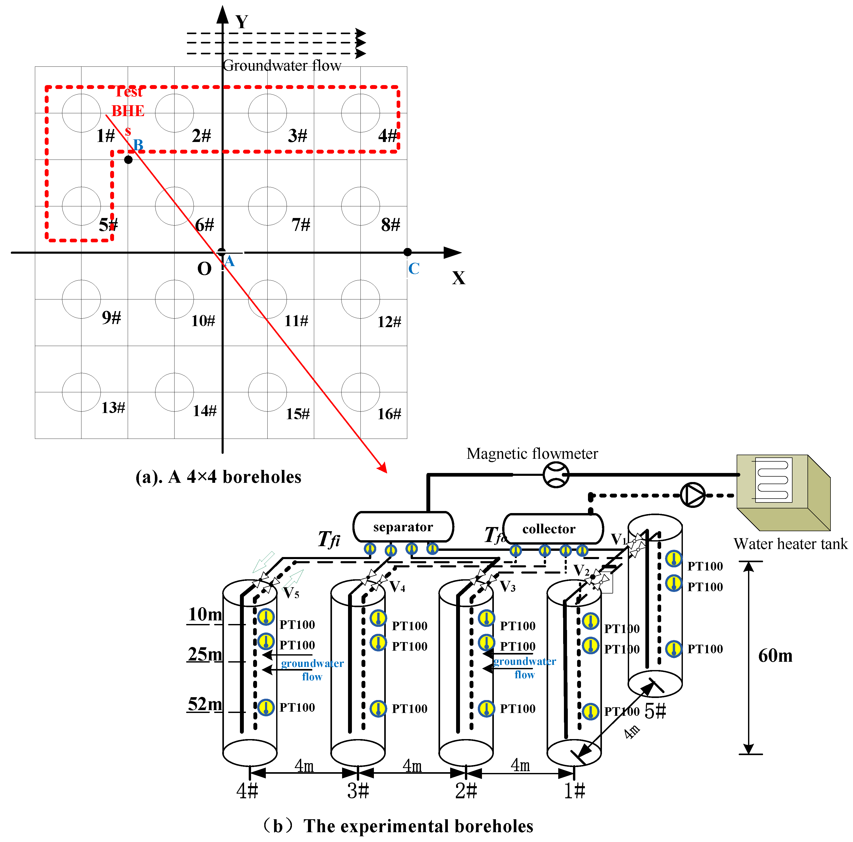
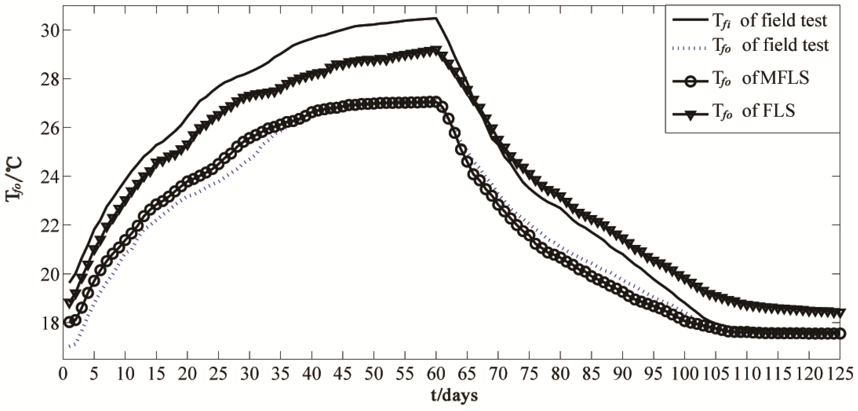
3. Experiential Study and Validation

A test and survey was conducted to analyze the performance of borehole heat transfer considering the effect of groundwater flow. The boreholes were bored at a hillside located in Zhushan, Nanjing, China. The area is in the middle and lower reaches of the Yangtze River, and the boreholes are frequently drilled in water-saturated undergrounds. A 4 × 4 boreholes field 60 m deep were drilled to supply the cooling for a small hotel, as shown in Figure 1a. In order to facilitate the test, the boreholes 1#, 2#, 3#, 4#, and 5# shown in Figure 1b were taken as studied objects. The PT100 temperature sensors were installed at the outlet and inlet of the borehole and at a depth of 10 m, 25 m, and 52 m in borehole-1#, 2#, 3#, 4#, and 5#. Combined with the early geologic exploration, it indicates that the main direction of the groundwater flow in the site is from borehole -1# to borehole -2#, shown in Figure 1b. The experiential system flow diagram is shown in Figure 1. The groundwater flow was found between the depth of 8 m and 56 m, the soil–rock sample indicated that the geological formation was almost silt and gravel, with high permeability. This zone was considered to be an aquifer.

In Figure 1b, the heating water was circulated through borehole-1#, 2#, 3#, 4#, and 5# for 60 days, and was followed by a 65 days self-recovery period. With the aid of the related parameters in

Table 1. Parameters of BHEs.

Parameter	Symbol	Unit	Value
undisturbed soil temperature	Tgr	[℃]	16.5
borehole diameter	db	[m]	0.20
branch pipe outer diameter	dp	[m]	0.032
pipe thickness	δ	[m]	0.0025
Shank spacing	xc	[m]	0.064
grout thermal conductivity	λg	[W/m.K]	2.4
grout vol. heat capacity	ρgcg	[J/m3/K]	3.2 × 106
soil thermal conductivity	λs	[W/m.K]	2.0
soil vol. heat capacity	ρscs	[J/m3/K]	4.8 × 106
pipe thermal conductivity	λp	[W/m.K]	0.6
borehole length	H	[m]	60
heat flux per unit length	qL	[W/m]	30
groundwater flow velocity	u	[m/s]	2 × 10−7
porosity	φ	-	0.25

, the measured mass flow rate and inlet temperature are used as input values for the MFLS multi-BHEs model (Equation 5). The FLS model ignoring the groundwater flow was also calculated to compare with the MFLS multi-BHEs model. The thermal load accounted for variable heat injection rates by calculating the flow rate and the inlet and outlet temperature. Figure 2 compared the experimentally measured outlet temperatures of the five boreholes field with the outlet temperature calculated by FLS and MFLS models.

Figure 2 shows that the performance of the multi-BHEs was underestimated by the FLS model, which neglects the influence of groundwater flow. For instance, the outlet temperature of the FLS was 0.8 ℃ higher than the tested outlet temperature at the 10^th day, and the temperature difference extended to 1.9 ℃ by the 60^th day. Also during the self-regeneration period, the outlet temperature from the FLS was 1.2 ℃ higher than the tested outlet temperature on the 80^th day. The error of the estimation was significantly reduced by using the moving finite line model (MFLS). The maximum deviations in the outlet temperature of the MFLS multi-BHEs model compared to the experiment were 0.23 ℃ and 0.25 ℃ on the 30^th day and on the 75^th day, respectively. It shows a very good match of the MFLS model with the field experimental data. It indicates that the groundwater would greatly influence on the performance and thermal recovery ability of the BHEs field.

4. Analysis of Dynamic Cooling Load Models for Multi-BHEs

Based on the MFLS Multi-BHEs model, a 4 × 4 boreholes field was arranged in a fixed grid, as illustrated in Figure 3. The field was selected to analyze how the groundwater flow influences the temperature field of multi-BHEs. The typical points A (0, 0), B (‒4, 4), and C (8, 0) were chosen to discuss the temperature response under different load models and optimized strategies.

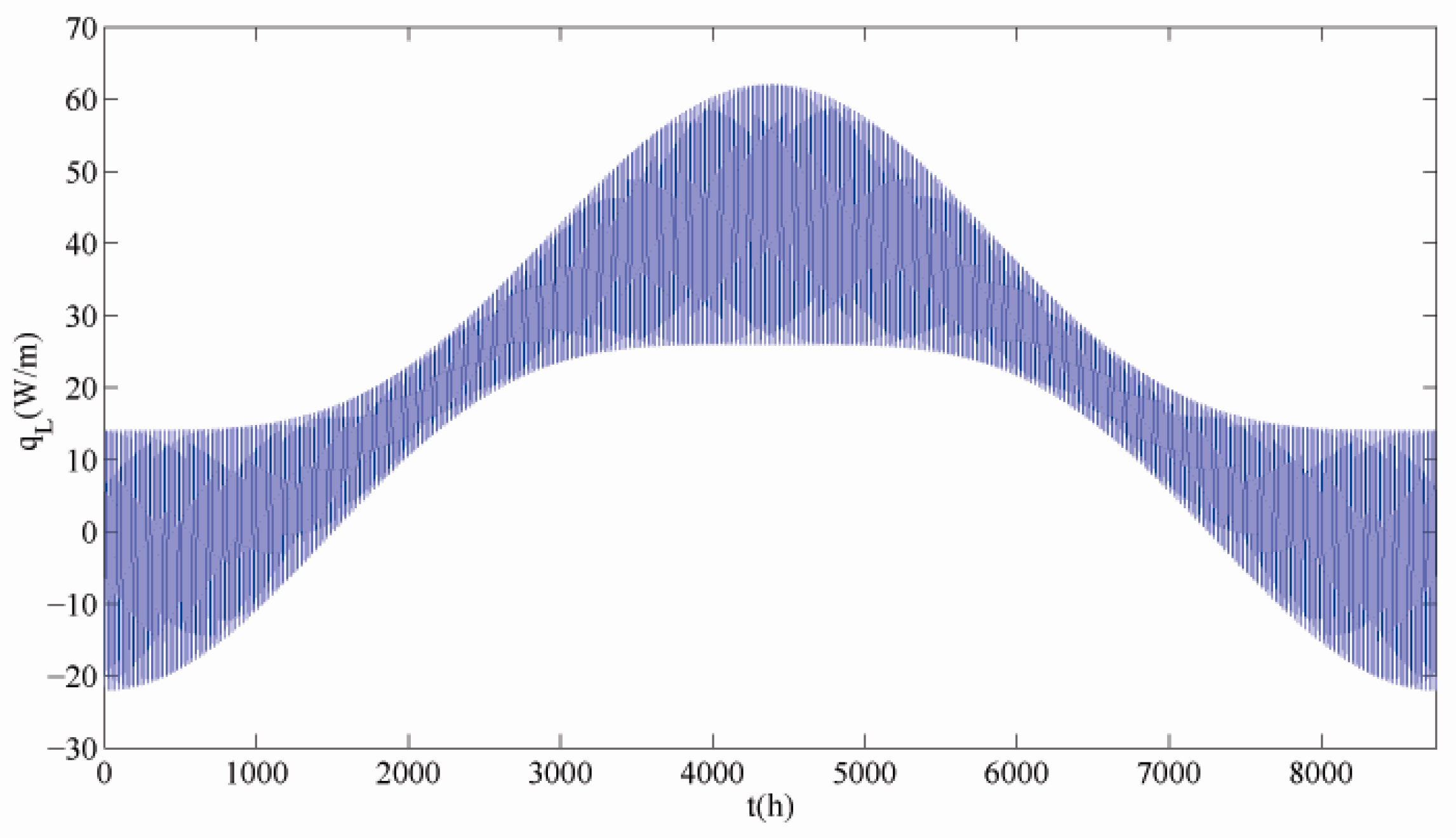
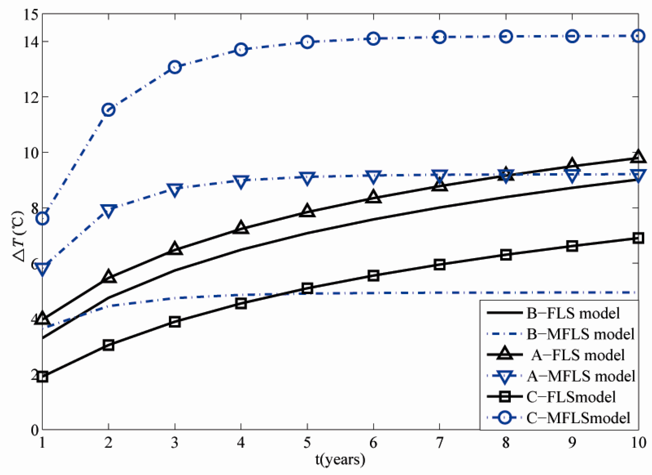
4.1. Long-term Analysis under an Annual Load Pattern

To analyze how the annual load pattern influences the thermal response of BHEs with long-term running time, a periodic cooling load per unit length with a regular cosine shape and period of one year is assumed for an individual borehole. The loads model function is shown as Equation (6):

$$q_L=p_1-p_2\cos (\frac{t}{8760}2\pi )-p_3\cos (\frac{t}{24}2\pi )-p_4\cos (\frac{t}{24}2\pi )\cos (\frac{t}{8760}2\pi )$$

(6)

where t is in hours, P₁ controls the annual load imbalance; P₂ is the half-amplitude of the annual load variation; P₃ and P₄ control the half-amplitude of daily load fluctuations. P₄/P₃ controls the relative importance of the damped component used to simulate relatively larger daily fluctuations during winter and summer.

The annual load scenario was considered with P₂ = 24, P₃ = 12, and P₄ = 6. The case was approximately balanced (P₁ = 20), and the annual load dynamic variation is depicted in Figure 4. Based on the MFLS multi-BHEs model, the analysis performed in this part considered a time interval of 10 years, and was thus called annual load dynamic variation analysis. With the aid of the parameters in Table 1, assuming the groundwater flow as u = 2 × 10⁷m/s. Figure 5 gives the temperature rise of typical points A, B, and C (Figure 3) for 10 years using the finite and moving finite line source models.

In Figure 5, based on the FLS model, the temperature rise of the control point can be seen to be strongly related to the positions in the boreholes field. The nearer to the center of the boreholes field is, the higher the temperature rise of the control point. After the 8^th year, the temperature of the central point A is 0.5 ℃ and 1.6 ℃ higher than the temperature rise of the points B and C, respectively. Furthermore, the temperature rise increased slowly in the non-groundwater multi-BHEs field. Nevertheless, even after ten years running, the temperature was still rising. This is due to that the FLS model, leading to smaller heat exchange rate between the borehole and the subsurface, and the heat accumulation nearby the borehole with the running time increasing. The heat exchange capacity of the soil gradually dropped.

Based on the MFLS model, on the other hand, the temperature rise at different control points taking into account the effects of groundwater flow could be obtained based on the MFLS model. Figure 5 shows that the temperature in the downstream locations was significantly larger than that in the upstream location. This agrees with the research done by Hecht-Mendez et al. [31]. After 5 years, the temperature of the control point C was 13.8 ℃, which was 6 ℃ and 7.6 ℃ higher than the temperature rise of the points A and B, respectively. Compared to the temperature rise at point B of the MFLS model and the FLS model, it could be found that the rate of temperature rising of the MFLS model was larger than that of the FLS model during the initial stage. But the rate decreased with time, and eventually decreased to zero after 5 years. The temperature of the MFLS model at point B was lower than that of the FLS model after 8 years. It indicates that the groundwater flow caused the heat to spread farther to avoid the heat accumulation nearby the borehole, although the heat accumulated downstream along the groundwater flow. It also implies that the thermal interaction between two neighboring boreholes would become complex because of the groundwater flow. Therefore, the design of the distance between the boreholes and the optimization of the BHEs field must carefully consider the effects of groundwater.

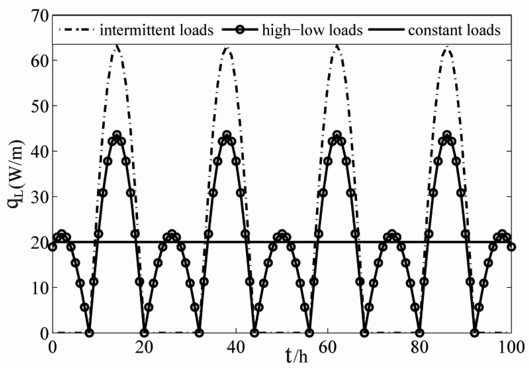
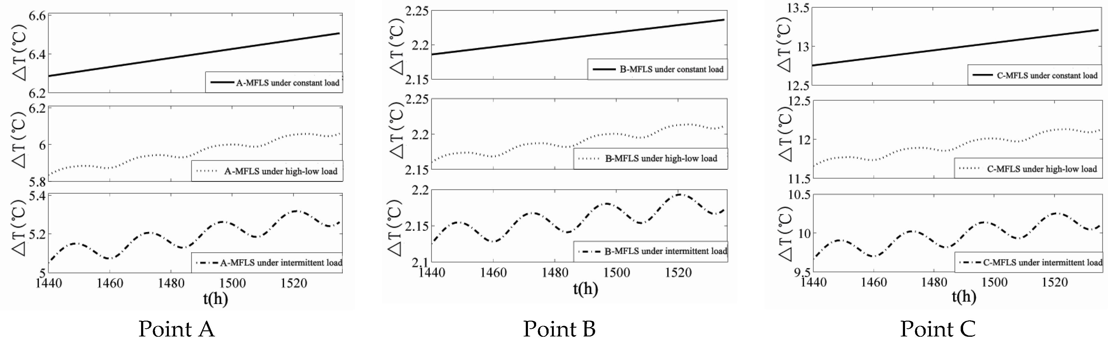
4.2. Short-term Analysis under Dynamic Diurnal Load Models

The diurnal variation of the building cooling load results in a periodic load per unit length of the individual borehole for the BHEs field. Considering the dynamic diurnal variation of the cooling load, this part of the study is devoted to the evaluation of the temperature rise of control point A (0, 0), B (‒4, 4), and C (8, 0) in the 4 × 4 BHEs field shown in Figure 3.

The building dynamic diurnal variation of the cooling load was injected into the ground by the circulating fluid. Three dynamic diurnal load models were considered, including constant load, dynamic intermittent load, and day-high night-low load models, respectively, represented by Equation (7), Equation (8), and Equation (9) as:

• Constant load model

  $$q_L=A_p$$

  (7)
• Intermittent load model

  $$q_L=\frac{1}{2}{A}_{pj}\sin (\frac{t-8}{24}2\pi )+\frac{1}{2}{A}_{pj}\left|\sin (\frac{t-8}{24}2\pi )\right|$$

  (8)
• Day-high night-low load model

  $$q_L=\frac{1}{4}{A}_{pg}\sin (\frac{t-8}{24}2\pi )+\frac{3}{4}{A}_{pg}\left|\sin (\frac{t-8}{24}2\pi )\right|$$

  (9)

  where A_p, A_pj, A_pg represent the positive or negative heat flux per unit length of the three load models, (W/m), such that the absolute values of A_p, A_pj, A_pg are the highest magnitude of the cooling load per unit length every day.

In this work, the same amounts of heat 4.8 kW were injected into the individual borehole (borehole depth H = 60 m) under the three diurnal load models. Based on Equation (7), Equation (8), and Equation (9), A_p = 20 W/m, A_pj = 63.18 W/m, and A_pg = 43.63 W/m. The three dynamic diurnal cooling load models are shown in Figure 6.

With the aid of the parameters in Table 1, substituting Equation (7), Equation (8), and Equation (9) into the MFLS multi-BHEs model of Equation (5), the temperature rise of the multi-BHEs field under the three diurnal load models could be obtained. Figure 7 gives the temperature rise variation of typical points A, B, and C (Figure 3) between 1440 h and 1536 h.

From Figure 7, after 1500 h of operation under the intermittent load model, the temperature rise of the downstream point C was 9.8 ℃, which was 4.6 ℃ and 7.7 ℃ higher than the temperature rise of the points A and B, respectively. It indicates that there were extreme temperature anomalies downstream in the multi-BHEs field.

Comparing the temperature rise in the multi-BHEs field of the three different diurnal load models, the temperature rise difference was very small under the different load models at the upstream point B. This is due to the fact that the heat in the upstream diffused to the downstream side with the groundwater flow. However, the temperature rise was different under different diurnal load models in the midstream and the downstream. The temperature rise of point A was 6.3 ℃ after 1440 h under the constant load model; it was 0.5 ℃ and 1.1 ℃ higher than the temperature rise of the day-high night-low load and intermittent load models, respectively.

When taking the groundwater flow in account, the groundwater flow made the heat spread farther and lead to temperature anomalies in the downstream BHEs field. The different diurnal load models could alleviate the heat accumulation in the downstream BHEs field to some extent. The intermittent diurnal load model could reduce the temperature rise in the downstream BHEs field. Compared to the constant load model, the temperature rise of point C under the intermittent load model was 2.8 ℃ lower after 1500 h.

5. Optimization for Multi-BHEs

5.1. The Optimization Model

Zeng et al. [6] developed a quasi three-dimensional model for BHEs based on the heat capacity of the materials inside the borehole, and the short-circuiting between legs, for a single U-tube borehole, the dimensionless energy equilibrium equation is expressed as Equation (10) with the dimensionless parameters listed in

Table 2. Dimensionless parameters.

Dimensionless Parameters	Dimensionless Parameters
${\mathrm{\Theta }}_1(z)=\frac{T_{f1}(z)-T_b}{T_{in}-T_b}$ ${\mathrm{\Theta }}_2(z)=\frac{T_{f2}(z)-T_b}{T_{in}-T_b}$ $R_{12}=\frac{1}{2\pi {\lambda }_g}[\ln (\frac{r_b}{2x_c})+\frac{{\lambda }_g-{\lambda }_s}{{\lambda }_g+{\lambda }_s}\ln (\frac{r_b{}^2}{r_b{}^2-x_c{}^2})]$	$Z=\frac{z}{H}$ $R_{11}=R_{22}=\frac{1}{2\pi {\lambda }_g}[\ln (\frac{r_b}{r_p})+\frac{{\lambda }_g-{\lambda }_s}{{\lambda }_g+{\lambda }_s}\ln (\frac{r_b{}^2}{r_b{}^2-x_c{}^2})]+R_p+R_f$ $R_1{}^{*}=\frac{\dot{m}c{R}_1{}^{\Delta }}{H}$
$R_2{}^{*}=\frac{\dot{m}c{R}_2{}^{\Delta }}{H}$ $R_{12}{}^{*}=\frac{\dot{m}c{R}_{12}{}^{\Delta }}{H}$ $R_1{}^{\Delta }=R_2{}^{\Delta }=\frac{R_{11}{R}_{12}-R_{12}{}^2}{R_{22}-R_{12}}$ $R_{12}{}^{\Delta }=\frac{R_{11}{R}_{12}-R_{12}{}^2}{R_{12}}$ $\beta =\sqrt{\frac{1}{4}{(\frac{1}{R_1{}^{*}}+\frac{1}{R_2{}^{*}})}^2+\frac{1}{R_{12}{}^{*}}(\frac{1}{R_1{}^{*}}+\frac{1}{R_2{}^{*}})}$
$f_1(z)=ch(\beta z)-\frac{1}{\beta }(\frac{1}{R_1{}^{*}}+\frac{1}{R_{12}{}^{*}})sh(\beta z)$ $f_2(z)=\frac{1}{\beta }\frac{1}{R_{12}{}^{*}}sh(\beta z)$ $f_3(z)=ch(\beta z)+\frac{1}{\beta }(\frac{1}{R_1{}^{*}}+\frac{1}{R_{12}{}^{*}})sh(\beta z)$

Note: Tf1(z), Tf2(z) are the fluid temperature of downward and upward legs of the tubes in the borehole, respectively.

.

$$\{\begin{array}{l}\partial {\mathrm{\Theta }}_1/\partial z={\mathrm{\Theta }}_1/R_1{}^{*}+({\mathrm{\Theta }}_1-{\mathrm{\Theta }}_2)/R_{12}{}^{*}\\ \partial {\mathrm{\Theta }}_2/\partial z={\mathrm{\Theta }}_2/R_1{}^{*}+({\mathrm{\Theta }}_1-{\mathrm{\Theta }}_2)/R_{12}{}^{*}\end{array}$$

(10)

with dimensionless boundary conditions: ${\mathrm{\Theta }}_1(0)=1$; ${\mathrm{\Theta }}_1(1)={\mathrm{\Theta }}_2(1)$.

The Laplace transform inverse transform were applied to Equation (10) to derive the dimensionless circulating fluid temperature along the borehole as shown in Equation (11):

$$\{\begin{array}{l}{\mathrm{\Theta }}_1(z)=f_1(z)+f_2(z)(f_1(1)+f_2(1))/(f_3(1)-f_2(1))\\ {\mathrm{\Theta }}_2(z)=-f_2(z)+f_3(z)(f_1(1)+f_2(1))/(f_3(1)-f_2(1))\end{array}$$

(11)

Several authors [31,47,48] have presented optimizations by minimizing the existing maximal ground temperature differences. But the heat transfer inside the borehole and thermal short-circuiting between the downward leg of the pipe and the upward leg of the pipe [51] is neglected in these methods. The optimization model combining heat transfer inside the borehole and outside the borehole would produce a more accurate estimation of the magnitude of the thermal anomalies. In this section, the optimization was proposed based on a procedure given by de Paly et al. [52] Beck M et al. [47] for cooling only cases. The efficiency of the heat pump of a geothermal installation is mainly influenced by the fluid temperature coming from the BHE field T_fo. For a given energy demand, maximum efficiency is achieved if the maximum outlet temperature is kept to the minimum. In this paper, we chose the T_fo as optimization targets. Therefore in the cooling case, it is reasonable to keep max (T_fo) as low as possible to keep the maximum outlet temperature caused by the heat injection through the BHEs as small as possible and to mitigate extreme temperature anomalies, and by this, ultimately improve heat pump performance.

With the aid of the multi-BHEs model presented in Equation (5) and the quasi 3D model of the circulating fluid into BHEs given in Equation (11), an optimization function is formulated as:

$$\mathrm{minimize}(\max (\Delta T_{f{o}_{i,j}}))$$

(12)

T_{fo i,j} is the outlet temperature on the position (i ,j) at time step t with the inlet temperature T_{fi i,j}. The T_{fo i,j} could be calculated by combining the MFLS multi-BHEs model and quasi 3D model.

Considering the entire time period t, we get for the outlet temperature minimization:

$$\text{arg min}(\max (\Delta T_{f{o}_{i,j}}(t,T_{f{i}_{i,j}})))\begin{array}{cc}& \forall (i,j,t)\end{array}\in S$$

(13)

In order to minimize the temperature changes within each of the single time steps l, a secondary optimization criterion is needed, which considers the maximum temperature change at each time step l:

$$\arg \min ({\displaystyle \sum _{l=1}^m\max (\Delta T_{f{o}_{i,j}}(l,T_{f{i}_{i,j}}))})\begin{array}{cc}& \forall (i,j,t)\end{array}\in S$$

(14)

Both optimization criteria can be combined using a weighted sum

$$\arg \min (w\cdot \max (\Delta T_{f{o}_{i,j}}(t,T_{f{i}_{i,j}})+{\displaystyle \sum _{l=1}^m\max (\Delta T_{f{o}_{i,j}}(l,T_{f{i}_{i,j}}))})\begin{array}{cc}& \forall (i,j,t)\end{array}\in S$$

(15)

where w is a weighting factor which should be set to a large value to ensure the priority of the primary objective over the secondary objectives. w was set to 85 in this study.

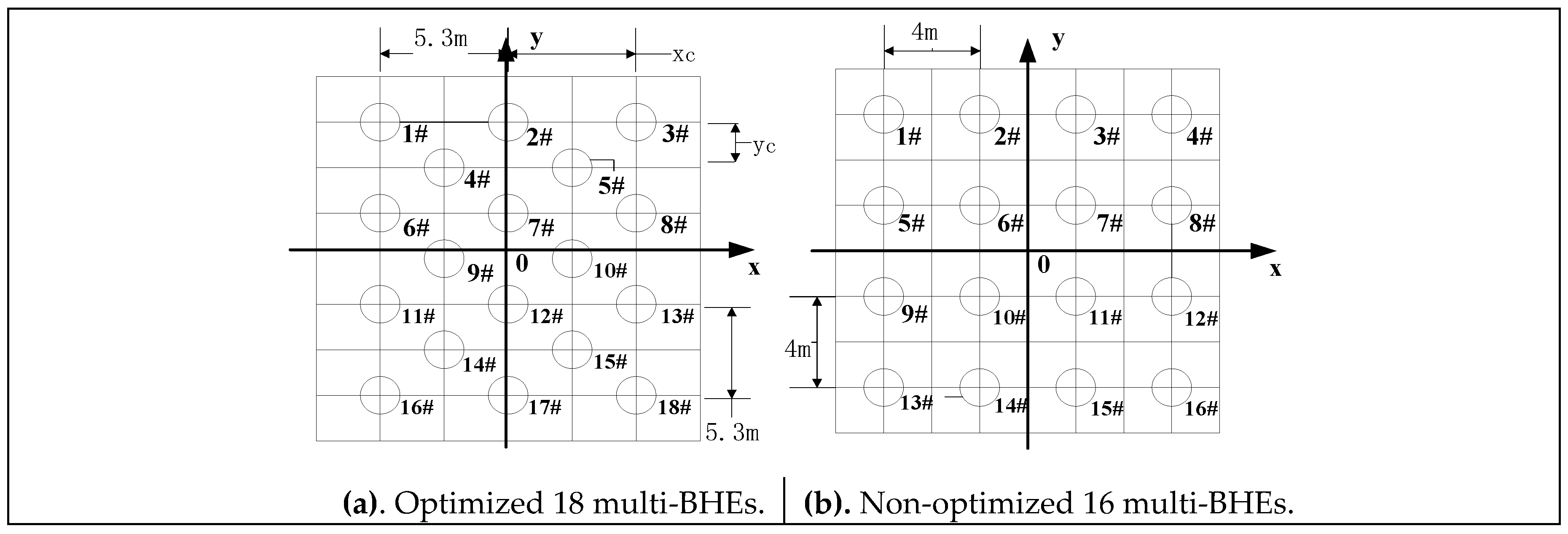
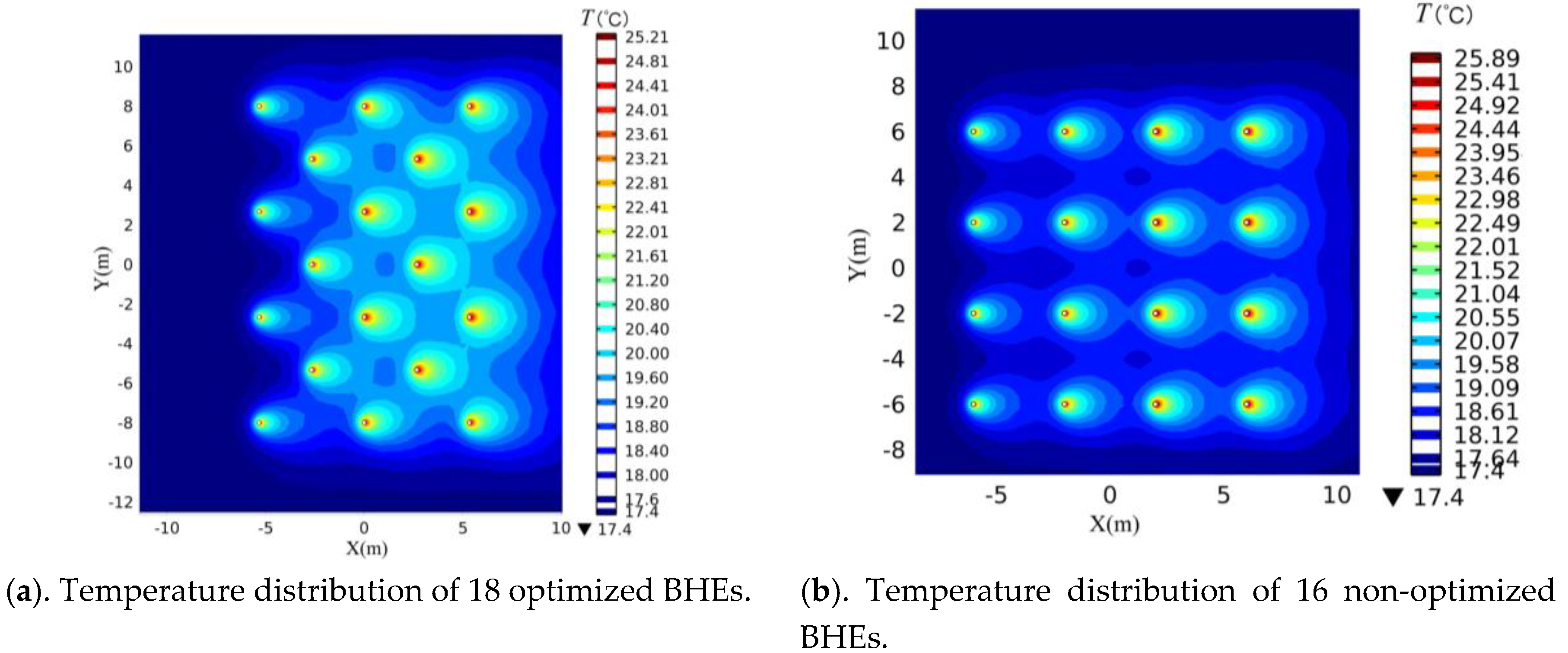
5.2. Application of Optimization-Arrangement Optimization

Free space in an urban area is diminishing day by day and limited space is available for drilling boreholes. Therefore, optimization of a BHEs arrangement is an important research topic that, by considering the groundwater flow, should ensure the maximum heat transfer capacity from soil. The main purpose of the arrangement optimization is maximum utilization of the heat transfer capacity of the multi-BHEs in a certain area for drilling.

The average temperature of the multi-BHEs field could be calculated as:

$$\overline{T_{\mathrm{s}}}=({\displaystyle \iint \theta {(x,y,z,t)}_{MFLS}dxdy)}/S$$

(16)

The arrangement optimization was done in a square of 16 × 16 m² in Figure 3. The number of the boreholes n, the horizontal spacing x_c = x_j+1-x_j, and longitudinal spacing y_c = y_j+1-y_j between boreholes were taken as the control objectives. Considering the far field condition, the square area for finite element numerical simulation was set as 25 × 25 m². The borehole depth is 60 m, and the soil and grout thermal parameters are shown in Table 1. The inlet temperature is set as 32 ℃. The load (heat transfer rate per unit length) for each borehole q_j was assumed be equal. The optimization procedure were used to find the optimized arrangement for multi-BHEs. The optimized arrangement and a non-optimized arrangement for multi-BHEs are shown in Figure 8.

The number of optimized multi-BHEs in Figure 8a is 18 with a horizontal spacing x_c = 5.3 m and longitudinal spacing y_c = 2.65 m. The non-optimized arrangement is a 4 × 4 square lattice arrangement shown in Figure 8b. Through the arrangement optimization, the number of boreholes increases from 16 to 18. The utilization ratio of the allowable area could be improved by 12.5%.

Figure 9 showed the temperature distribution of the optimized 18 multi-BHEs and non-optimized 16 multi-BHEs with the groundwater velocity (Pe = 1.26) u = 2 × 10^-7 m/s after 90 days of running.

In Figure 9, it showed that the optimized soil average temperature was about 1.0 ℃ lower than that of the non-optimized fields. This indicates that the optimized multi-BHEs have a larger heat transfer performance. Moreover, the temperature of point C (8, 0) was only 1.75 ℃ higher than the temperature of point A (0, 0) in the optimized BHEs fields, as shown in Figure 9a. On the other hand, the difference between temperature rises at points C and A was 2.6 ℃ in the non-optimized BHEs fields, shown in Figure 9b. Therefore, the arrangement optimization could mitigate temperature anomalies in the downstream BHEs fields and could make full use of the soil heat transfer performance.

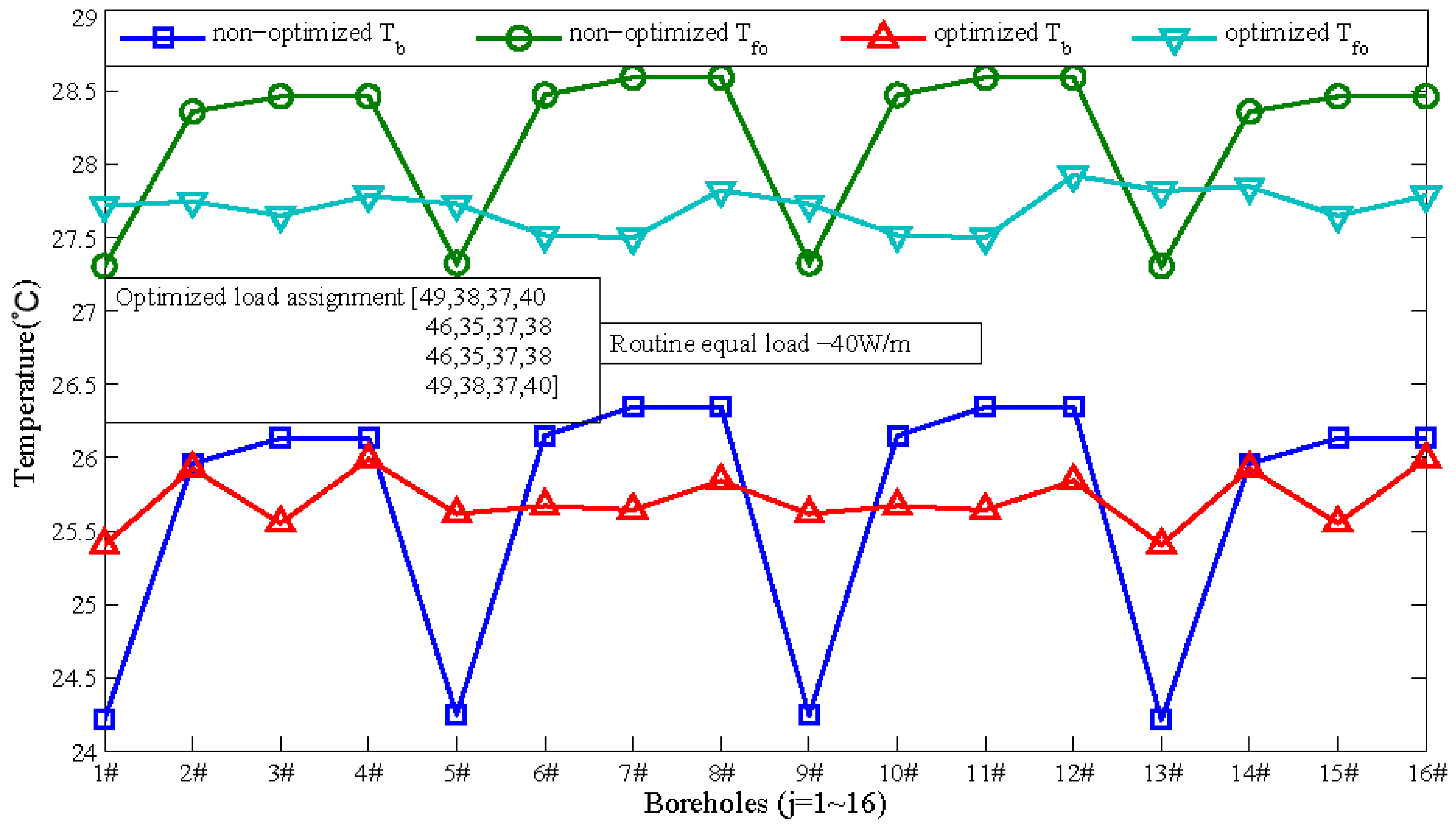
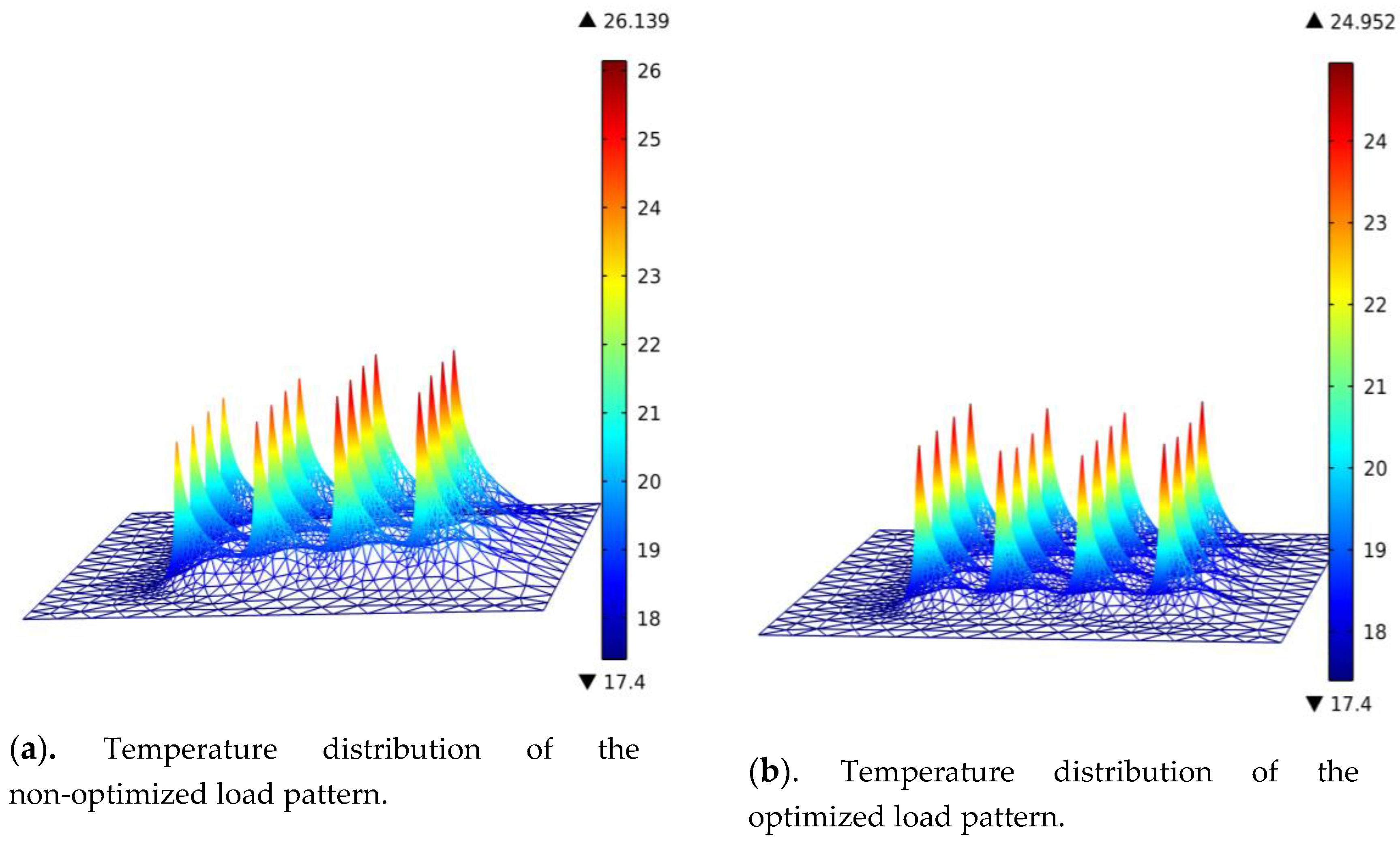
5.3. Application of Optimization-Load Optimization

Generally, the load for every borehole is equal, and multiple BHEs are operated in parallel, with equal flow velocity of the circulating carrier fluid. Considering the groundwater flow, the equal load assignment would lead to temperature anomalies in the downstream BHEs field. The heat transfer efficiency of the downstream BHEs field would become lower with time for the temperature anomalies, but the upstream BHEs could not exert their heat exchange capacities. Through the optimal load assignment for each borehole, the ground temperature in a BHE field was, to some extent, automatically balanced, and substantial local temperature anomalies were thus mitigated by smaller heat extraction from cold regions.

For given geometric arrangements of BHEs, the load assigned to each BHE was taken as the control objective.

The rate of temperature imbalance for multi-BHEs (η) in Equation (17) was introduced as a secondary optimization function. It was used to discuss the local temperature anomalies of the multi-BHEs.

$$\eta =\frac{\Delta T_{\max }(x,y)-\Delta T_{\min }(x,y)}{T_{ground}}$$

(17)

where △T_max(x,y) and △T_min(x,y) are maximum temperature rise and minimum temperature rise in the multi-BHEs fields, respectively.

The 16 BHEs, initially arranged in a square lattice, as shown in Figure 3, were optimized through the optimal load assignment. Soil thermal parameters were used, as listed in Table 1. The distance between the BHEs was 4 m (x_c = y_c = 4 m). The given heat rejection load was given as 640 kW, with the runtime of 90 days. The non-optimal load pattern with equal load for each borehole means that the heat transfer rate of every BHEs was 40 W/m. The borehole temperature and the outlet temperature of optimized load and non-optimal practice were compared, as shown in Figure 10. The temperature distribution fields of the load optimized and non-optimized pattern are shown in Figure 11.

In Figure 10, after 90 days of running the non-optimized equal load assigned pattern, the borehole wall temperatures of first row boreholes (1#, 5#, 9#, 13#) were all below 24.3 ℃. However, the temperatures of the last row boreholes (4#, 8#, 12#, 16#) were all lager than 26.1 ℃. This resulted in 1℃ outlet temperature difference between the first row of BHEs and the last row of BHEs. Upon extrapolation, the difference would be 2.8 ℃ when the runtime was 365 days. The borehole wall temperature of borehole 8# and borehole 12# would be 31.8 ℃, which means there was almost no temperature difference between fluid inside the borehole and the borehole wall. For the optimized load pattern, the borehole wall temperature and outlet temperature of different boreholes were consistent. The borehole wall temperature of the downstream boreholes declined and the borehole wall temperatures of the upstream boreholes increased. The average outlet temperature of the load-optimized multi-BHEs was 27.70 ℃, which was 0.8 ℃ lower than that of the non-optimized load pattern.

In Figure 11, based on Equation (16), the average soil temperature of the load-optimized and non-optimal were 18.62 ℃ and 20.15 ℃, respectively. The optimized load model resulted in an average soil temperature decrease of 7.6%. The maximum temperature rise of the optimized and non-optimized temperature fields was 2.61 ℃ and 3.62 ℃, respectively. The minimum temperature rise of the optimized and non-optimized temperature fields was 0.35 ℃ and 0.04 ℃, respectively. Combined with Equation (17), the temperature unbalance rate η of the optimized and non-optimized temperature fields was 12.98% and 20.56%, respectively. Temperature unbalance rate η is reduced by 36.9% through the load optimization. This indicates that the local heat accumulation in BHEs fields can be reduced owing to the load optimization, thus ensuring improved long-term performance of the multi-BHEs.

6. Conclusions

The groundwater flow caused the thermal anomalies downstream. Considering the cooling case only, the soil temperature in the downstream is greatly larger than that of the upstream. This would lead to larger ground temperature differences in the multi-BHEs field and the ground field could not exert its overall heat exchanger efficiency. Based on the moving finite line source model, a heat transfer model was proposed for the soil of multi-BHEs fields by applying a superposition principle. The calculation results from a MFLS model and a FLS model were compared with the measured outlet temperatures from a field test for a borehole field. Based on the proposed MFLS multi-BHEs model, a 4 × 4 boreholes field was analyzed to examine how the groundwater flow affects the temperature field of multi-BHEs.

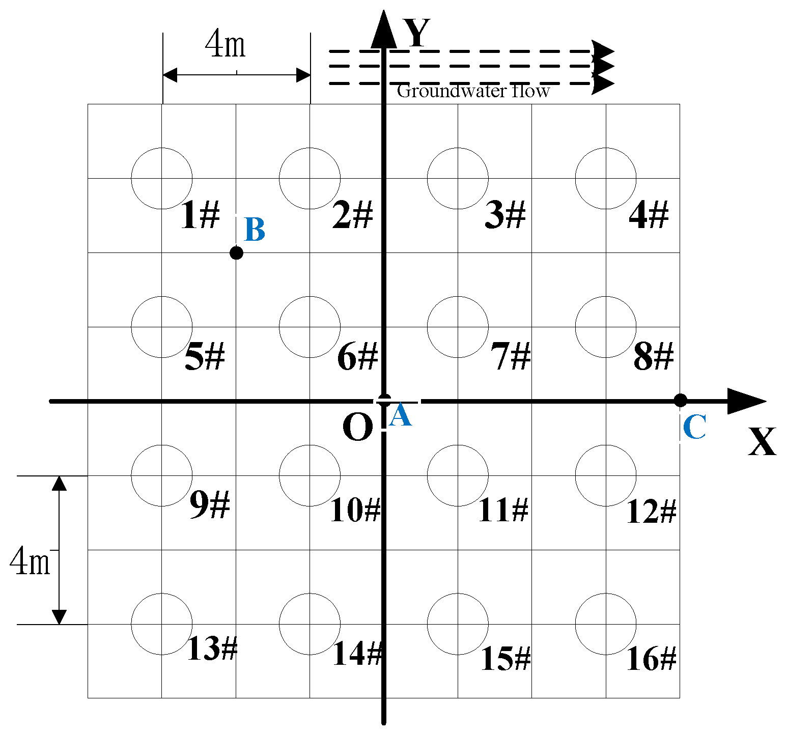
• The long-term performance of multi-BHEs fields under an annual dynamic load pattern was studied using the finite and the moving finite line source models. In the FLS model of a BHEs field, the rise in temperature increased from the far-field towards the center of the boreholes. In the MFLS model, the groundwater flow caused the heat to spread farther, and the heat accumulated in the downstream along the groundwater flow. For a field of 4 × 4 boreholes, the temperature rise of a downstream point was 13.8 ℃ after 5 years running, which was 6 ℃ higher than the temperature rise of the central point. It implies that the design of the distance between the boreholes and the optimization of the BHEs field must carefully consider the effects of groundwater.
• Three dynamic diurnal load models, including constant load, dynamic intermittent load, and day-high night-low load models, were considered to evaluate the temperature rise in the 4 × 4 BHEs field. Compared to the constant load model, the temperature rise of downstream point C under the intermittent load model was 2.8 ℃ lower after 15:00 h of running. When designing the multi-BHEs, the diurnal load models of different buildings should be carefully considered; this is because the different dynamic diurnal load models would lead to different characteristics of thermal anomalies.
• Combining with the MFLS multi-BHEs model with the quasi 3D model of the circulating fluid, an optimization model was established for multi-BHEs to minimize the average outlet circulating fluid temperature and to mitigate the temperature anomalies. The optimization model considering the fluid temperature variation and thermal short-circuiting between the downward leg of the pipe and the upward leg of the pipe inside the borehole would produce a more accurate estimation of the magnitude of the thermal anomalies.

The optimization for arrangement and the optimization for load were performed based on the proposed optimization model. The results showed that the optimization for arrangement could mitigate temperature anomalies in the downstream BHEs fields; the optimized average temperature of soil of the multi-BHEs fields was approximately 1.0 ℃ lower than of the non-optimized fields. In this paper, through the optimal load assignment for each borehole, the average outlet temperature of the optimized multi-BHEs was 0.8 ℃ lower than that of the non-optimized BHEs. The rate of temperature unbalance was reduced by 36.9% by using the load optimization.

References

1. Ingersoll, L.; Zobel, O.; Ingersoll, A. Heat Conduction with Engineering, Geological and Other Applications; McGraw-Hill: New York, NY, USA, 1954. [Google Scholar]
2. Deerman, J.D.; Kavanaugh, S.P. Simulation of vertical U-tube ground coupled heat pump systems using the cylindrical heat source solution. ASHRAE Trans. 1991, 97, 287–295. [Google Scholar]
3. Bernier, M.A.; Pinel, P.; Labib, R.; Paillot, R. A multiple load aggregation algorithm for annual hourly simulations of GCHP systems. Hvac R Res. 2004, 10, 471–487. [Google Scholar] [CrossRef]
4. Fossa, M.; Minchio, F. The effect of borefield geometry and ground thermal load profile on hourly thermal response of geothermal heat pump systems. Energy 2013, 51, 323–329. [Google Scholar] [CrossRef]
5. Eskilson, P.; Claesson, J. Simulation model for thermally interacting heat extraction boreholes. Number Heat Transf. 1988, 13, 149–165. [Google Scholar]
6. Zeng, H.Y.; Diao, N.R.; Fang, Z.H. A finite line-source model for boreholes in geothermal heat exchangers. Heat Transf. Asian Res. 2002, 31, 558–567. [Google Scholar] [CrossRef]
7. Lamarche, L. A fast algorithm for the hourly simulations of ground-source heat pumps using arbitrary response factors. Renew. Energy 2009, 34, 2252–2258. [Google Scholar] [CrossRef]
8. Bandos, T.V.; Montero, Á.; Fernández, E.; Santander, J.L.G.; Isidro, J.M.; Pérez, J.; Fernández de Córdoba, P.J.; Urchueguía, J.F. Finite line-source model for borehole heat exchangers: Effect of vertical temperature variations. Geothermics 2009, 38, 263–270. [Google Scholar] [CrossRef]
9. Yavuzturk, C.; Spitler, J.D. A short time step response factor model for vertical ground loop heat exchangers. ASHRAE Trans. 1999, 105, 475–485. [Google Scholar]
10. Michopoulos, A.; Kyriakis, N. Predicting the fluid temperature at the exit of the vertical ground heat exchangers. Appl. Energy 2009, 86, 2065–2070. [Google Scholar] [CrossRef]
11. Monzó, P.; Mogensen, P.; Acuña, J. A novel numerical model for the thermal response of borehole heat exchanger fields. In Proceedings of the 11th IEA heat pump conference, Montréal, QC, Canada, 12–16 May 2014.
12. Li, M.; Lai, A.C.K. Analytical model for short-time responses of borehole ground heat exchangers: Model development and validation. Appl. Energy 2013, 104, 510–516. [Google Scholar] [CrossRef]
13. Yang, Y.; Li, M. Short-time performance of composite-medium line-source model for predicting responses of ground heat exchangers with single U-shaped tube. Int. J Therm. Sci. 2014, 82, 130–137. [Google Scholar]
14. Li, M.; Li, P.; Chan, V.; Lai, A.C.K. Full-scale temperature response function (G-function) for heat transfer by borehole ground heat exchangers (GHEs) from sub-hour to decades. Appl. Energy 2014, 136, 197–205. [Google Scholar] [CrossRef]
15. Hu, P.; Zha, J.; Lei, F.; Zhu, N.; Wu, T. A composite cylindrical model and its application in analysis of thermal response and performance for energy pile. Energy Build. 2014, 84, 324–332. [Google Scholar] [CrossRef]
16. Lei, F.; Hu, P.F.; Zhu, N.; Wu, T.H. Periodic heat flux composite model for borehole heat exchanger and its application. Appl. Energy 2015, 151, 132–142. [Google Scholar] [CrossRef]
17. Zanchini, E.; Lazzari, S. New g-functions for the hourly simulation of double U-tube borehole heat exchanger fields. Energy 2014, 70, 444–455. [Google Scholar] [CrossRef]
18. Erol, S.; Hashemi, M.A.; François, B. Analytical solution of discontinuous heat extraction for sustainability and recovery aspects of borehole heat exchangers. Int. J. Therm. Sci. 2015, 88, 47–58. [Google Scholar] [CrossRef]
19. Mottaghy, D.; Dijkshoorn, L. Implementing an effective finite difference formulation for borehole heat exchangers into a heat and mass transport code. Renew. Energy 2012, 45, 59–71. [Google Scholar] [CrossRef]
20. Bauer, D.; Heidemann, W.; Diersch, J.G. Transient 3D analysis of borehole heat exchanger modeling. Geothermics 2011, 40, 250–260. [Google Scholar] [CrossRef]
21. Pasquier, P.; Marcotte, D. Joint use of quasi-3D response model and spectral method to simulate borehole heat exchanger. Geothermics 2014, 51, 281–299. [Google Scholar] [CrossRef]
22. Gehlin, S.E.A.; Hellstrom, G. Influence on thermal response test by groundwater flow in vertical fractures in hard rock. Renew. Energy 2003, 28, 2221–2238. [Google Scholar] [CrossRef]
23. Diao, N.; Li, Q.Y.; Fang, Z.H. Heat transfer in ground heat exchangers with groundwater advection. Int. J. Therm. Sci. 2004, 43, 1203–1211. [Google Scholar] [CrossRef]
24. Wang, H.J.; Qi, C.Y.; Du, H.P.; Gu, J.H. Thermal performance of borehole heat exchanger underground water flow: A case study from Baoding. Energy Build. 2009, 41, 1368–1373. [Google Scholar] [CrossRef]
25. Chiasson, A.; O’Connell, A. New analytical solution for sizing vertical borehole ground heat exchangers in environments with significant groundwater flow: Parameter estimation from thermal response test data. Hvac&R Res. 2011, 17, 1000–1011. [Google Scholar]
26. Molina-Giraldo, N.; Blum, P.; Zhu, K.; Bayer, P.; Fang, Z.H. A moving finite line source model to simulate borehole heat exchangers with groundwater advection. Int. J. Therm. Sci. 2011, 50, 2506–2513. [Google Scholar] [CrossRef]
27. Angelotti, A.; Alberti, L.; Licata, I.; Antelmi, L.M. Energy performance and thermal impact of a Borehole Heat Exchanger in a sandy aquifer: Influence of the groundwater velocity. Energy Convers. Manag. 2014, 77, 700–708. [Google Scholar] [CrossRef]
28. Rivera, J.A.; Blum, P.; Bayer, P. Analytical simulation of groundwater flow and land surface effects on thermal plumes of borehole heat exchangers. Appl. Energy 2015, 146, 421–433. [Google Scholar] [CrossRef]
29. Zanchini, E.; Lazzari, S.; Priarone, A. Long-term performance of large borehole heat exchanger fields with unbalanced seasonal loads and groundwater flow. Energy 2012, 38, 66–77. [Google Scholar] [CrossRef]
30. Capozza, A.; De Carli, M.; Zarrella, A. Investigations on the influence of aquifers on the ground temperature in ground-source heat pump operation. Appl. Energy 2013, 107, 350–363. [Google Scholar] [CrossRef]
31. Hecht-Mendez, J.; de Paly, M.; Beck, M.; Bayer, P. Optimisation of energy extraction for vertical closed-loop geothermal systems considering groundwater flow. Energy Convers. Manag. 2013, 66, 1–10. [Google Scholar] [CrossRef]
32. Dagdas, A. Heat exchanger optimization for geothermal district heating systems: A fuel saving approach. Renew. Energy 2007, 32, 1020–1028. [Google Scholar] [CrossRef]
33. Desideri, U.; Sorbi, N.; Arcioni, L.; Leonardi, D. Feasibility study and numerical simulation of a ground source heat pump plant, applied to a residential building. Appl. Therm. Eng. 2011, 31, 3500–3510. [Google Scholar] [CrossRef]
34. Herbert, A.; Arthur, S.; Chillingworth, G. Thermal modelling of large scale exploitation of ground source energy in urban aquifers as a resource management tool. Appl. Energy 2013, 109, 94–105. [Google Scholar] [CrossRef]
35. Montagud, C.; Corberán, J.M.; Ruiz-Calvo, F. Experimental and modeling analysis of a ground source heat pump system. Appl. Energy 2013, 109, 328–236. [Google Scholar] [CrossRef]
36. Man, Y.; Yang, H.; Wang, J.; Fang, Z. In situ operation performance test of ground coupled heat pump system for cooling and heating provision in temperate zone. Appl. Energy 2012, 97, 913–920. [Google Scholar] [CrossRef]
37. Shang, Y.; Dong, M.; Li, S. Intermittent experimental study of a vertical ground source heat pump system. Appl. Energy 2014, 136, 628–635. [Google Scholar] [CrossRef]
38. Ally, M.R.; Munk, J.D.; Baxter, V.D.; Gehl, A.C. Exergy analysis of a two-stage ground source heat pump with a vertical bore for residential space conditioning under simulated occupancy. Appl. Energy 2015, 155, 502–514. [Google Scholar] [CrossRef]
39. Lazzari, S.; Priarone, A.; Zanchini, E. Long-term performance of BHE (borehole heat exchanger) fields with negligible groundwater movement. Energy 2010, 35, 4966–4974. [Google Scholar] [CrossRef]
40. Fan, R.; Jiang, Y.Q.; Yao, Y.; Shiming, D.; Ma, Z.L. A study on the performance of a geothermal heat exchanger under coupled heat conduction and groundwater advection. Energy 2007, 32, 2199–2209. [Google Scholar] [CrossRef]
41. Choi, J.C.; Park, J.; Lee, S.R. Numerical evaluation of the effects of groundwater flow on borehole heat exchanger arrays. Renew. Energy 2013, 52, 230–240. [Google Scholar] [CrossRef]
42. Rybach, L.; Eugster, W.J. Sustainability aspects of geothermal heat pump operation, with experience from Switzerland. Geothermics 2010, 39, 365–369. [Google Scholar] [CrossRef]
43. Man, Y.; Yang, H.X.; Spitler, J.D. Feasibility study on novel hybrid ground coupled heat pump system with nocturnal cooling radiator for cooling load dominated buildings. Appl. Energy 2011, 88, 4160–4171. [Google Scholar]
44. Allaerts, K.; Coomans, M.; Salenbien, R. Hybrid ground-source heat pump system with active air source regeneration. Energy Convers. Manag. 2015, 90, 230–237. [Google Scholar] [CrossRef]
45. Macíaa, A.; Bujedo, L.A.; Magraner, T.; Chamorro, C.R. Influence parameters on the performance of an experimental solar-assisted ground-coupled absorption heat pump in cooling operation. Energy Build. 2013, 66, 282–288. [Google Scholar] [CrossRef]
46. Yu, M.Z.; Zhang, K.; Cao, X.Z.; Hu, A.J.; Cui, P.; Fang, Z.H. Zoning operation of multiple borehole ground heat exchangers to alleviate the ground thermal accumulation caused by unbalanced seasonal loads. Energy Build. 2016, 110, 345–352. [Google Scholar] [CrossRef]
47. Beck, M.; Bayer, P.; de Paly, M.; Hecht-Méndez, J.; Zell, A. Geometric arrangement and operation mode adjustment in low-enthalpy geothermal borehole fields for heating. Energy 2013, 49, 434–443. [Google Scholar] [CrossRef]
48. Bayer, P.; De Paly, M.; Beck, M. Strategic optimization of borehole heat exchanger field for seasonal geothermal heating and cooling. Appl. Energy 2014, 136, 445–453. [Google Scholar] [CrossRef]
49. Zhang, W.; Yang, H.X.; Lu, L.; Fang, Z.H. The analysis on solid cylindrical heat source model of foundation pile ground heat exchangers with groundwater flow. Energy 2013, 55, 417–425. [Google Scholar] [CrossRef]
50. Rivera, J.A.; Blum, P.; Bayer, P. Ground energy balance for borehole heat exchangers: Vertical fluxes, groundwater and storage. Renew. Energy 2015, 83, 1341–1351. [Google Scholar] [CrossRef]
51. Li, Y.; Mao, J.F.; Geng, S.B.; Han, X.; Zhang, H. Evaluation of thermal short-circuiting and influence on thermal response test for borehole heat exchanger. Geothermics 2014, 50, 136–147. [Google Scholar] [CrossRef]
Figure 1. BHE (borehole) locations and experimential system flow diagram. (a) A 4 × 4 boreholes (b) The experimential boreholes.
Sustainability 08 00577 g001
Figure 2. Comparison of experimentally measured outlet temperatures with those from FLS (finite line source) and MFLS (moving finite line source) multi-BHEs models.
Sustainability 08 00577 g002
Figure 3. Grid arrangement of BHEs in an area of 16m × 16m. Coordinates:A (0, 0), B (‒4, 4), C (8, 0).
Sustainability 08 00577 g003
Figure 4. Annual load dynamic variation of BHE.
Sustainability 08 00577 g004
Figure 5. Temperature variation of typical points A, B, C with time.
Sustainability 08 00577 g005
Figure 6. The three models for the dynamic diurnal load variation.
Sustainability 08 00577 g006
Figure 7. Temperature rise of typical points under three different dynamic loads for the MFLS model.
Sustainability 08 00577 g007
Figure 8. Comparison between an optimized and a non-optimized arrangement.
Sustainability 08 00577 g008
Figure 9. Temperature distribution of the optimized and non-optimized arrangement multi-BHEs (z = 50 m).
Sustainability 08 00577 g009
Figure 10. The borehole wall and outlet temperature of each BHE between the load non-optimized and optimized pattern.
Sustainability 08 00577 g010
Figure 11. Temperature distribution of the load optimized and non-optimized multi-BHEs (z = 50 m).
Sustainability 08 00577 g011