Article

Drought Risk Assessment Based on Vulnerability Surfaces: A Case Study of Maize

1
School of Geography, Beijing Normal University, Beijing 100875, China
2
The Key Laboratory of Regional Geography, Beijing Normal University, Beijing 100875, China
3
China Insurance Information Technology Management Co., Ltd., Beijing 100144, China
4
The State Key Laboratory of Earth Surface Processes and Resource Ecology, Beijing Normal University, Beijing 100875, China
*
Author to whom correspondence should be addressed.
Sustainability 2016, 8(8), 813; https://0-doi-org.brum.beds.ac.uk/10.3390/su8080813
Submission received: 14 June 2016 / Revised: 3 August 2016 / Accepted: 11 August 2016 / Published: 18 August 2016
(This article belongs to the Special Issue Resilience to Natural and Man-Made Disasters)

Abstract

:
Agriculture is a sector easily affected by meteorological conditions. Crop yield reduction, even regional conflicts, may occur during a drought. It is extremely important to improve the state of our knowledge on agricultural drought risk. This study has proposed a new method (vulnerability surfaces) for assessing vulnerability quantitatively and continuously by including the environmental variable as an additional perspective on exposure and assessed global maize drought risk based on these surfaces. In this research, based on the Environmental Policy Impact Climate (EPIC) model, irrigation scenarios were adopted to fit “Loss rate-Drought index-Environmental indicator (L-D-E)” vulnerability surfaces by constructing a database suitable for risk assessment on a large scale. Global maize drought risk was quantitatively assessed based on its optimal vulnerability surface. The results showed an R2 for the optimal vulnerability surface of 0.9934, with coarse fragment content as the environmental indicator. The expected global average annual yield loss rate due to drought was 19.18%. The global average yield loss rate due to drought with different return periods (10a, 20a, 50a, and 100a) was 29.18%, 32.76%, 36.89%, and 38.26%, respectively. From a global perspective, Central Asia, the Iberian Peninsula, Eastern Africa, the Midwestern United States, Chile, and Brazil are the areas with the highest maize drought risk. The vulnerability surface is a further development of the vulnerability curve as a continuous expression of vulnerability and considers differences in environmental factors. It can reflect the spatial heterogeneity of crop vulnerability and can be applied in large-scale risk assessment research.

Graphical Abstract

1. Introduction

The Intergovernmental Panel on Climate Change (IPCC) 5th Assessment Report confirmed that, in general, global temperatures rose from 1880 to 2012, with a linear trend of 0.85 °C/100a. Temperature increases are therefore expected to characterize global climate change in the 21st century. By the end of the 21st century, the global average temperature will have increased by at least 1.5 °C compared with the period from 1850 to 1900 [1]. The probability of severe and persistent droughts may increase in the future under the influence of climate change and anthropogenic forcing [2,3]. Droughts may bring about food security problems or even regional conflicts [4]. Agriculture is dependent on climate conditions and is greatly influenced by climate change [5,6]. Reducing drought risk has therefore become an important topic in disaster risk research and is critical for promoting global food security and sustainable agricultural development.
Risk assessment can generally be divided into hazard assessment and vulnerability assessment [7]. A number of drought indicators have been proposed for crop drought hazard assessment, such as the Palmer Drought Severity Index (PDSI) [8], the Standardized Precipitation Index (SPI) [9], the Vegetation Health Index (VHI) [10], and the Agricultural Reference Index for Drought(ARID) [11]. More recently, with the development of fuzzy mathematics in risk assessment [12], the quantitative evaluation of drought hazard has been generalized [13,14]. The most commonly and widely used methods of vulnerability assessment can be classified into three types: (1) vulnerability assessment based on historical disaster data, such as long-term data on precipitation, crop yield, and other factors [15,16,17]; (2) vulnerability assessment based on indicators [18,19,20]; and (3) vulnerability assessment based on the hazard–loss curve (also called the vulnerability curve), which can reflect the response of crop yield to drought from the aspects of crop physical properties [21,22,23]. Generally, case studies using the first two approaches may be limited if no long-term observational data are available. In addition, the first two methods provide only a qualitative or semi-quantitative vulnerability assessment. Risk assessment models also suffer from this limitation, and, as a result, they cannot directly estimate the probability of disaster losses [24]. A quantitative evaluation of crop vulnerability is clearly important to the quantitative assessment of agricultural drought risk [25]. The vulnerability curve can establish the quantitative functional relationship between hazard and loss. It provides a new method for quantitative evaluation of agricultural drought risk.
Vulnerability curves first appeared in 1964 [26] and were used to provide a quantitative measurement of the interaction between hazard intensity and corresponding loss (loss rate) [27]. A vulnerability curve can quantitatively evaluate crop vulnerability. Studies have used the water requirement satisfaction index (WRSI) and loss rate to produce maize drought vulnerability curves for three countries (Kenya, Malawi, and Mozambique) [28]. With the development and application of crop models in disaster science, crop drought vulnerability assessments have adopted these models [22,29]. Yin [30] fitted maize drought vulnerability curves for 35 regions globally, using the water stress index and a maize yield loss rate simulation with the EPIC model. Agricultural drought risk assessment based on vulnerability curves calculates the losses (or loss rates) at different hazard intensities and is hence more quantitative and accurate than risk level evaluations based on indicators.
However, the vulnerability curve involves only two dimensions, hazard intensity and loss, without considering environmental factors. Crop drought, however, is often influenced by more than just hazard intensity, which may vary among different environments. It is also difficult for vulnerability curves to express the continuous spatial variability of vulnerability. As a result, the spatial accuracy of risk assessment is limited, but can be improved by constructing a three-dimensional risk assessment method that includes loss rate, hazard intensity, and an environmental indicator. Surfaces have been commonly used for vulnerability assessments in earthquake disaster studies, in which fragility surfaces were fitted according to degree of damage and hazard intensity based on the structure of buildings or bridges. Lee [31] combined snow and earthquake hazards, both of which influence buildings, to fit fragility surfaces. Wang [32] considered the multiple hazards of earthquake and scour (flood and debris flow) to fit the fragility surface for a bridge. To date, few researchers have applied vulnerability surfaces to agricultural drought risk assessment. In fact, crop vulnerability varies among different locations. The evaluation under one environmental condition may not necessarily be applicable to other environments. The larger a study area, the greater is the variation in vulnerability, and the more important it becomes to fit continuous surfaces to express crop vulnerability.
In this paper, a method of fitting three-dimensional vulnerability surfaces (“Loss rate-Drought index-Environmental indicator (L-D-E)”) is proposed. This method may provide a new way to evaluate crop vulnerability by considering exposure that vulnerability curves could not cover. This paper also assesses global maize drought risk quantitatively based on vulnerability surfaces.

2. Materials and Methods

2.1. Basic Idea and Research Framework

2.1.1. Assessment of Physical Vulnerability to Maize Drought

The vulnerability of a system to climate change may be characterized as a function of the exposure, sensitivity, and adaptive capacity of the system [33]. Vulnerability is dynamic and complex and may vary with changes in both the biophysical and socioeconomic characteristics of a particular region. Biophysical vulnerability is an inherent attribute of the exposure or inventory, which can reflect the response of the crop to the disaster [22].
Further work is needed to integrate information about exposure, sensitivity, and adaptability to provide more detailed and quantitative information about the potential impacts of climate change and the relative degree of vulnerability of different regions, nations, and socioeconomic groups [33]. (1) Sensitivity is the degree to which a system is affected, either adversely or beneficially, by climate-related stimuli. The effects may be direct (e.g., a change in crop yield in response to a change in the mean, range, or variability of temperature) or indirect (e.g., damage caused by increased frequency of coastal flooding due to sea-level rise) and can be expressed by vulnerability curves; (2) Adaptation is the process of adjustment to actual or expected climate and its effects. In some natural systems, human intervention may facilitate adjustment to expected climate and its effects. In this study, human intervention (i.e., adaption, e.g., the possibilities for improvement of maize species, cultivation management, and other social factors) was not calculated as an influence index, but was considered as constant for lack of quantitative data; (3) Exposure is the presence of people, livelihoods, species or ecosystems, environmental functions, services, and resources, infrastructure, or economic, social, or cultural assets in places and settings that could be adversely affected [34]. In this study, location (planting area of maize) was assumed to be unchanged because it was difficult to simulate accurately.
Overall, only the biophysical aspect of vulnerability was considered, and the adaptability and sensitivity of maize were assumed to be constant. Therefore, irrigation scenarios were set by changing the amount of irrigation in the crop model. According to the output of the model (water stress and yield) under different irrigation scenarios, 3D surfaces considering environmental factors (settings) were fitted.

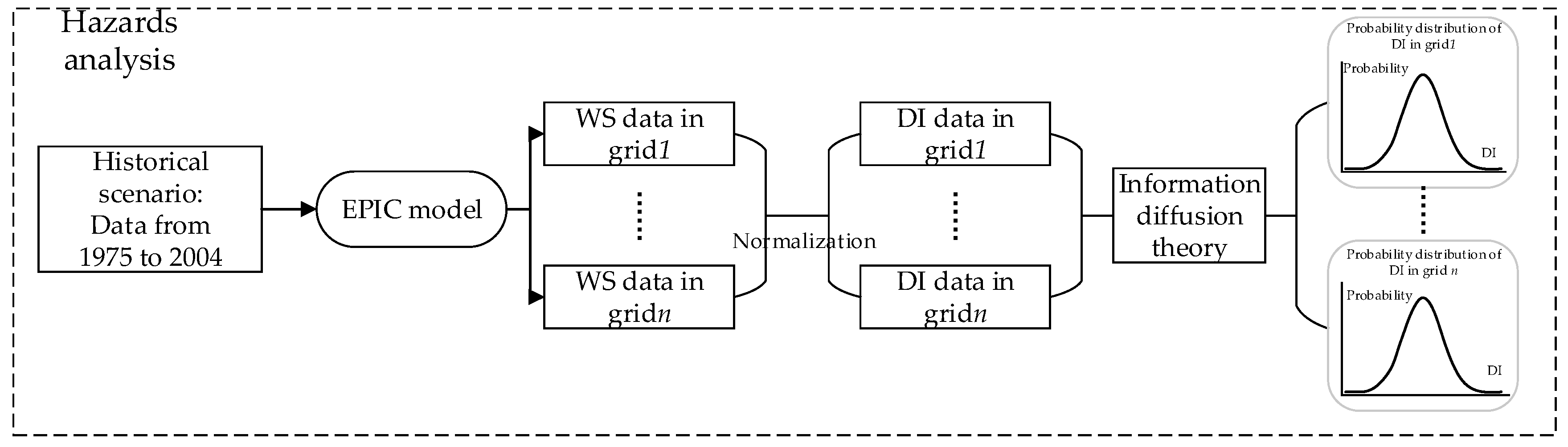
2.1.2. Assessment of Drought Intensity and Risk Based on Crop Model Simulation

With the development of crop models, many researchers have combined crop model simulation output with historical data and established indices to forecast drought risk [21,35]. This research suggests that a complex crop model can simulate the relationship between drought and crop productivity. In this study, yield and water stress index were simulated by the EPIC model. EPIC is a comprehensive model consisting mainly of hydrological, meteorological, erosion, nutrient cycling, soil temperature, crop growth, tillage, and economic modules. It can continuously simulate the growth processes of more than 100 kinds of crops using a daily time step and readily available inputs [36]. Productivity under climate change can be simulated effectively based on the model parameters and meteorological data.
In this research, water stress indices (WS) were simulated to evaluate water insufficiency for the drought intensity calculation. The meteorological data used in the EPIC model contain observational data from 1971 to 2004 and forecast data calculated by the Global Climate Model (GCM) [37]. To reduce the uncertainty of the model prediction, the section of observation data from 1975 to 2004 was chosen for this study. The WS index over 30 years in each grid cell was simulated all over the world based on the data. Information diffusion theory was used to calculate the probability distribution of drought intensity from a few WS samples. The pattern of drought intensity in different regions can be expressed based on the calibrated model. The calculated risk is the result of both drought intensity assessment and vulnerability assessment and is defined in this paper as the probability of a given loss rate of maize yield.

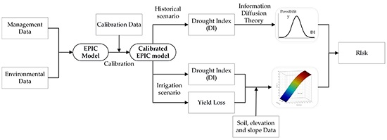
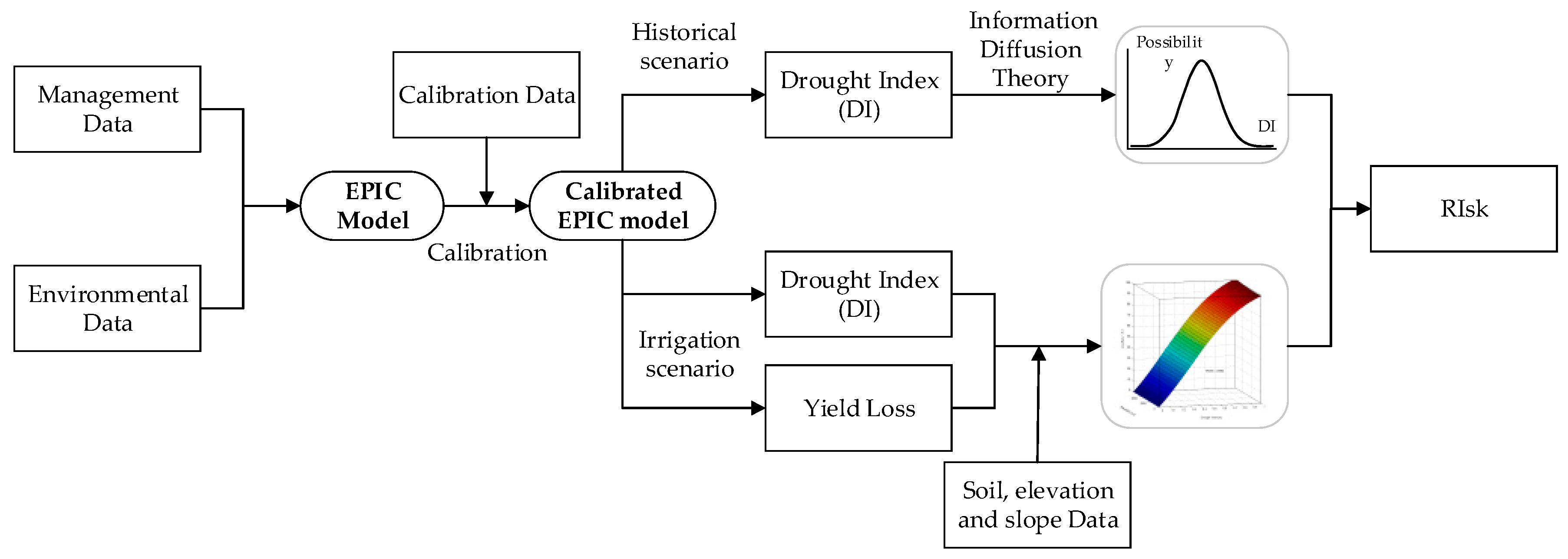
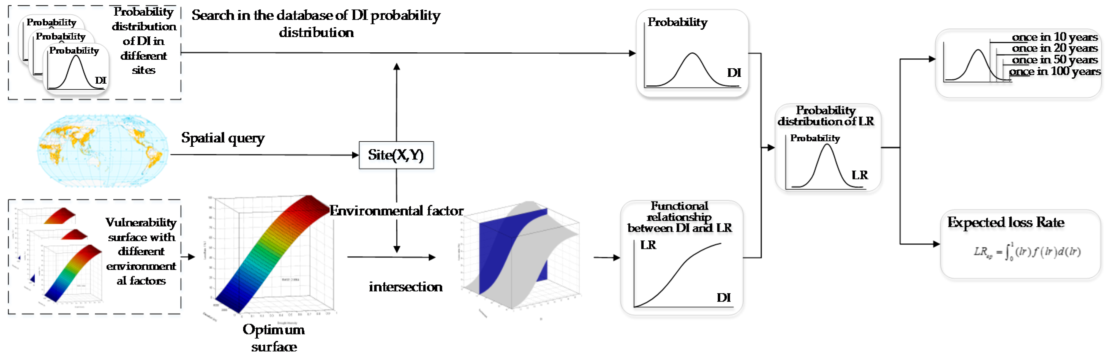
2.1.3. Research Framework

The study was conducted in three steps. In Step 1, an EPIC model was calibrated by adjusting several important parameters. In Step 2, based on the calibrated EPIC model, other variables were controlled, and different irrigation scenarios were defined to obtain yields and water stress indices (WS), which were normalized as yield loss rate (LR) and drought index (DI) respectively. LR, DI, and environmental indicators (E) (such as elevation, slope, and soil parameters) were combined to obtain vulnerability surfaces. In Step 3, historical data and the information diffusion theory were used to obtain the probability distribution of DI, which was combined with the vulnerability surface to calculate risk (considered to be the probability of LR) (Figure 1).

2.2. Data

The data were divided into three categories: geographical environment data, field management data, and calibration data (Table 1).
The geo-environmental data included global DEM, global slope [47], global soil parameters [48], and global meteorological [37] data as well as global data on the planting extent of maize [49]. The meteorological data contained daily data from 1971 to 2099 and consisted of actual meteorological observations from 1971 to 2004 and forecast data based on global climate model from 2005 to 2099. Daily values of maximum temperature, minimum temperature, precipitation, solar radiation, wind speed, and relative humidity were used in the EPIC model to assess the probability distribution of DI. Field management data included the growth period of global maize [50], global agricultural irrigation patterns [51], and global fertilizer application [52]. The irrigation and fertilizer data were defined as “maximum annual irrigation volume allowed” and “maximum annual nitrogen fertilizer application” for a crop respectively when running the EPIC model. The automatic options for fertilization and irrigation were applied in the EPIC model because it was impossible to obtain real fertilizer and irrigation schedules for each grid cell.
The EPIC model requires all input data to have the same spatial resolution. Hence, the spatial resolutions of all data were converted into the same resolution as the meteorological data.
The calibration data were the statistical yield of maize reported by FAO for each country (region) from 2000 to 2004, of which the data for 2000 were used to calibrate the model and the 2001–2004 data were used to validate it.

2.3. Methodology

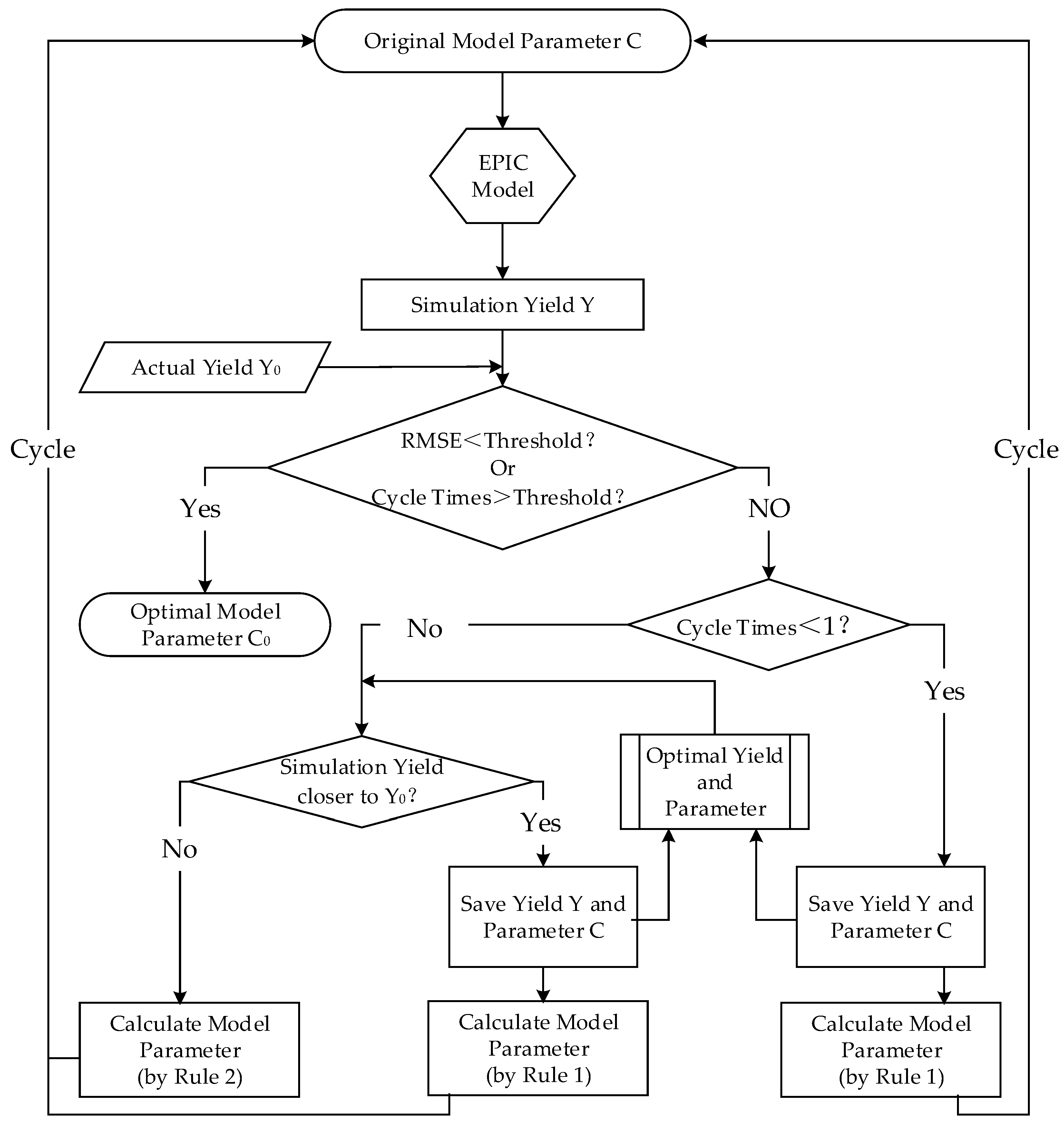
2.3.1. Calibration of EPIC

Model calibration is the basis for accurate simulation. For this study, risk was calculated by simulating the LR of maize yield under drought conditions produced by the EPIC model. Hence, it was important to simulate yield accurately. Moreover, the EPIC model parameters needed to be adjusted to suit different regions. The basic unit selected was the 0.5° × 0.5° grid, which is ideal for calibrating the model in each grid cell. However, when the model is calibrated in each grid cell, the cost of the calculation should be considered. Therefore, the country (region) was selected in this research as the basic unit to calibrate the EPIC model.
Based on earlier studies [53,54,55,56], four parameters (WA (biomass-energy ratio), HI (harvest index), DLMA (maximum potential leaf area index), and DLAI (fraction of the growing season when leaf area declines)) were considered as key parameters of the EPIC model. In the calibration process, the parameters were adjusted for each country (region) that was considered as a homogeneous unit to create a suitable EPIC model. The parameters of each grid cell in each unit were adjusted at the same time (hence, each grid cell in a unit has the same parameters). Simulated yields of 2000 in each grid cell were obtained with the EPIC model and averaged in each unit to be compared with the statistical yield of each country (region). When the simulated yields of 2000 were close to the statistical yields, the calibration was completed. The results of model calibration for each unit were evaluated by comparing simulated maize yields with statistical yields for 2001–2004.
Direction and step length are key factors in parameter adjustment. This study used the automatic adjustment method. The adjustment of each parameter in one unit can be described as three main steps.
Step 1: define the default value of each parameter as the initial value in each unit. Simulate the yield of each grid cell using the initial value, and calculate the average yield of each unit. Calculate the RMSE between the simulated and statistical yields. Consider the initial parameter value as the optimum value if the RMSE is less than the threshold.
Step 2: if the RMSE value is not less than the threshold, the parameter adjustment phase will work. First, consider the default value as the optimal parameter value and adjust it using Rule 1 if the number of cycles is less than 1.
Step 3: carry out a new judgment if the condition in Step 2 is not satisfied. Assuming that the N-th cycle is the current cycle, adjust the parameter using rule 1 if the simulated yield in the (N-1)-st cycle is closer than that in the (N-2)-nd cycle to the actual yield, or adjust it using Rule 2 if not.
Cycle through the adjustment process in the manner described above until the simulation results reach the output condition or the maximum number of cycles is reached; the optimal output parameters are assumed to be obtained (Figure 2).

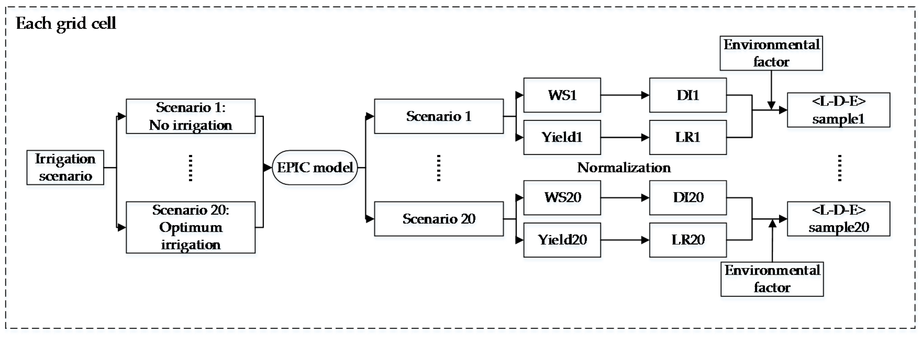
2.3.2. Fitting of the Vulnerability Surface

Based on the “Loss rate-Drought index-Environmental indicator (L-D-E)” samples generated by the calibrated EPIC model, the drought vulnerability surface of maize had three dimensions.
Water stress (WS) is an EPIC output factor that represents water shortage for plants. The value of WS ranges from 0 to 1; the higher the value, the more yield is affected by drought. Twenty irrigation scenarios were defined to obtain “L-D-E” samples. First, the optimal level of irrigation (there are no significant changes in yield when the irrigation level is continuously increased) was determined by pre-testing. Second, the single-variable method was used to keep the growth period, fertilizer addition rate, and meteorological data constant while varying the amount of irrigation to obtain WS and yield under different irrigation scenarios. Twenty irrigation scenarios were defined to control the amount of irrigation, which uniformly increased from 0 to the optimal value in each grid cell. Third, WS and yield were simulated by EPIC under each scenario and then normalized to DI and LR. In this way, 20 samples of DI and LR were calculated in different grid cells that had different environmental conditions. DI and LR were then combined with the environmental indicators for each grid cell to generate the “L-D-E” samples (Figure 3).
WS can be normalized by Equations (1) and (2):
D I k = H I max ( H I )
H I = i   =   1 n ( W S i ) ,
where WSi indicates the WS of maize on day i, n is the number of days that maize was influenced by WS in a growth period, HI is the accumulated value of WS in one maize growth period, max(HI) is the maximum value of HI under all irrigation scenarios, DIk is the hazard index in grid cell k, and k is the grid cell identification number.
Yield can be normalized using Equation (3):
L R = max ( y ) y max ( y ) ,
where y is the yield under one scenario, LR is the yield loss rate caused by drought, and max(y) is the maximum yield.
Two topographic indicators (elevation and slope) and seven soil indicators (coarse fragment content (CFRAG), bulk density (BULK), water content at field capacity (TAWC), sand content (SDTO), silt content (CLPC), organic carbon concentration (TOTC), and soil pH (PH)) were selected as environmental indicators for the study.
Twenty “L-D-E” samples for each grid cell were generated to fit a maize drought vulnerability surface with DI as the x-axis, an environmental indicator as the y-axis, and LR as the z-axis. The vulnerability surface was fitted by trend surface analysis (Equation (4)):
L R   =   ( a / ( 1 + b × e x p ( c × D I ) ) a / ( 1 + b ) ) ( a / ( 1 + b × e x p ( c ) ) a / ( 1 +   b ) ) × ( d × ( E e ) 2 + f ) ,
where LR is the maize yield loss rate, DI is the hazard index, E is an environmental factor, and a, b, c, d, e, f are parameters.

2.3.3. Drought Risk Assessment Based on the Vulnerability Surface

Risk assessment can generally be divided into hazard assessment and vulnerability assessment [7]:
R i s k = H a z a r d × V u l n e r a b i l i t y ,
where Risk is the maize drought risk, Hazard is the function of maize drought hazard, and Vulnerability is the function of maize drought vulnerability. Section 2.3.2 introduced the method of vulnerability assessment. Hazard was assessed using a three-step process: (1) historical data (30 years (1975–2004)) were used to establish WS for different grid cells using the EPIC simulation; (2) WS was normalized to DI (using a method similar to Equation (2)) to generate 30 years of DI samples for each grid cell; (3) the probability distribution of DI for different grid cells was obtained to complete the hazard assessment using information diffusion theory [57,58] (Figure 4).
In this research, DI samples over 30 years were found to be insufficient to estimate the probability distribution in each grid cell. Information diffusion theory provides a method to change observations into normal fuzzy sets so that the probability distribution of DI can be calculated. The basic principle of information diffusion theory was explained by Huang [12,57].
Let U = {u1, u2, u3, …, un} be a discrete universe of DI that contains its possible values. According to the definition of DI, the maximum value of U is 1, and the minimum is 0. In this study, the resolution of the discrete universe is 0.0001. Therefore, U = {0, 0.0001, 0.0002, …, 1}. The information carried by DI was therefore diffused to ui in each grid cell using the information diffusion function shown in Equation (6):
f k ( u i ) = 1 h 2 π exp [ ( D I k u i ) 2 2 h 2 ] ,
where k is the grid cell identification number and h is called the normal diffusion coefficient and is calculated by Equation (7):
h = { 0.8146 ( b a ) , 0.5960 ( b a ) , 0.4560 ( b a ) , 0.3860 ( b a ) , 0.3362 ( b a ) , 0.2986 ( b a ) , 2.8651 b a n 1 , | m = 5 m = 6 m = 7 m = 8 m = 9 m = 10 m 11 ,
where b is the maximum value of DI, a is the minimum, and m is the number of samples. In this paper, m is 30 in each grid cell.
Information accumulation can be calculated using Equations (8) and (9):
C k = i   =   1 n f k ( u i )
F ( D I k , u j ) = f k ( u j ) C k ,
where Ck is the information accumulation of the k-th sample and F(DIk,uj) is the normalized information distribution of sample DI. For each point uj, summing all normalized information, the information gain at uj, which came from the given sample DI, was obtained. The information gain is shown in Equation (10):
q ( u j ) = j   =   1 m F ( D I i , u j ) .
The diffusion information of the sample was obtained by summing q(uj) (Equation (11)):
Q = j   =   1 n q ( u j ) .
Next, the occurrence probability of a drought disaster of magnitude uj was estimated so that the probability distribution of DI could be assessed:
p ( u j ) = q ( u j ) Q .
Based on the probability distribution of DI and the vulnerability surface, the global maize drought risk was assessed (Figure 5).
The optimal surface with the highest R2 was chosen to assess the global drought risk for maize. For each grid cell, a pair of coordinates (x,y) was determined by a spatial query based on the overall planting extent of maize. According to the coordinates, the DI probability distribution curve of the grid cell was also identified. The function relating DI and LR was obtained by the intersection of E (an environmental indicator) and the optimal vulnerability surface. The function was then combined with the probability distribution of DI to calculate the probability distribution of LR for the grid cell. According to the probability distribution of LR, which represents the probability of different levels of LR, the expected risk was calculated. The LR risk at different return periods could also be obtained, where the probability of a 10a, 20a, 50a, and 100a return period corresponds to 0.1, 0.05, 0.02, and 0.01, respectively.

3. Results

3.1. Calibration Results

By comparing the simulated and actual yields (from FAO statistics) for the national (regional) units from 2001 to 2004, scatter plots were drawn, and a correlation analysis was completed (Figure 6).
Both actual and simulated global maize yields are concentrated in the vicinity of the 1:1 line. All R2 values are greater than 0.7. The Pearson correlation coefficients between simulated and actual yields from 2001 to 2004 were 0.898, 0.867, 0.857, and 0.860, respectively, and were significant at the 0.01 level. It can be seen that simulated yields are significantly correlated with actual yields, meaning that the model calibration result is positive.

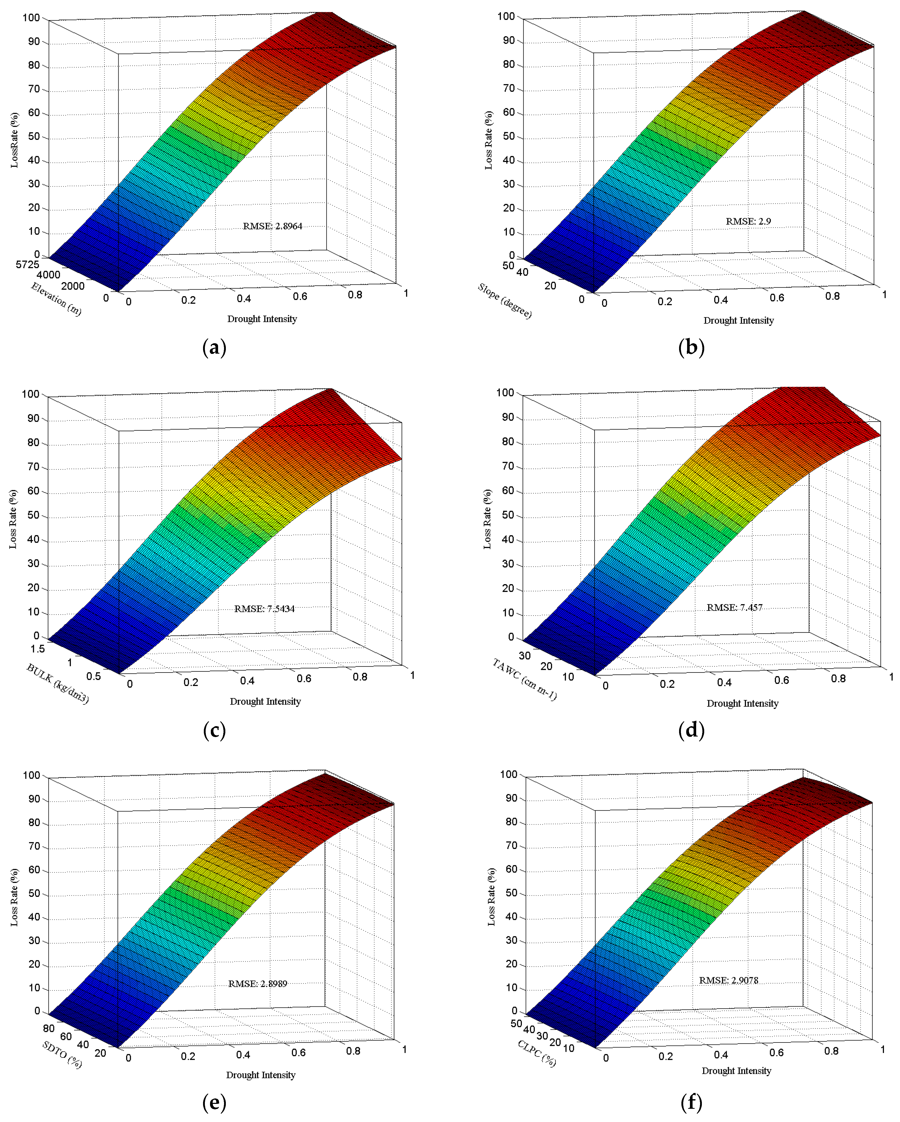
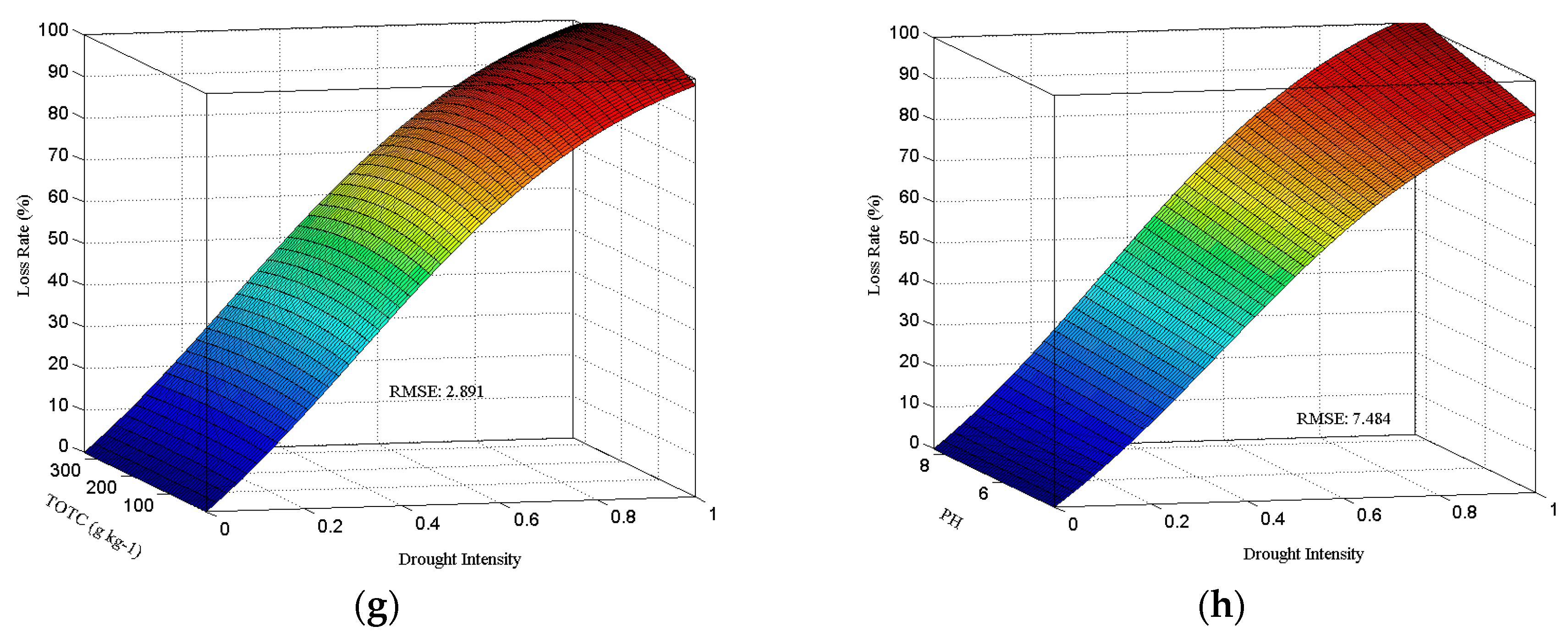
3.2. “L-D-E” Vulnerability Surface of Maize

Elevation, slope, and seven soil properties (CFRAG, BULK, TAWC, SDTO, CLPC, TOTC, and PH) were selected as environmental indicators to fit the drought vulnerability surface of maize (Table 2). Table 2 shows that the surface-fitting accuracy is generally good. The vulnerability surface with CFRAG as the environmental indicator has the best fitting accuracy, with an R2 of 0.99342 and an RMSE of 2.89062.
According to the optimal vulnerability surface (Figure 7) for global maize, under the same CFRAG, LR rises significantly with an increase in DI. When DI does not change, LR decreases at first, reaching a minimum when CFRAG is approximately 10%, and then increases.

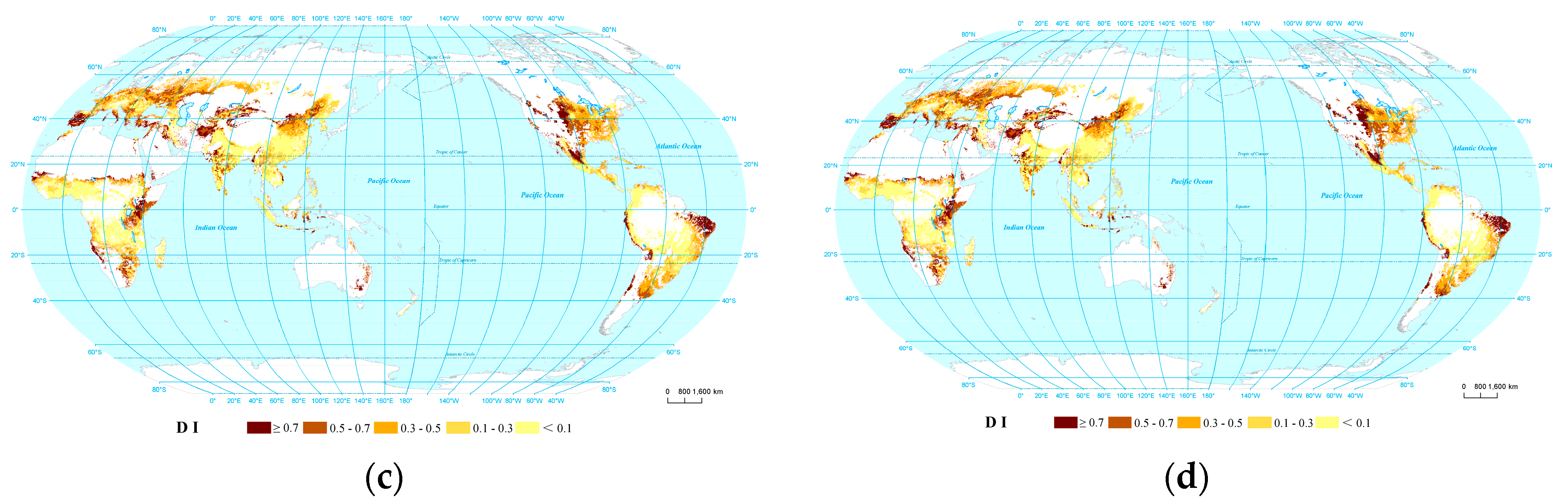
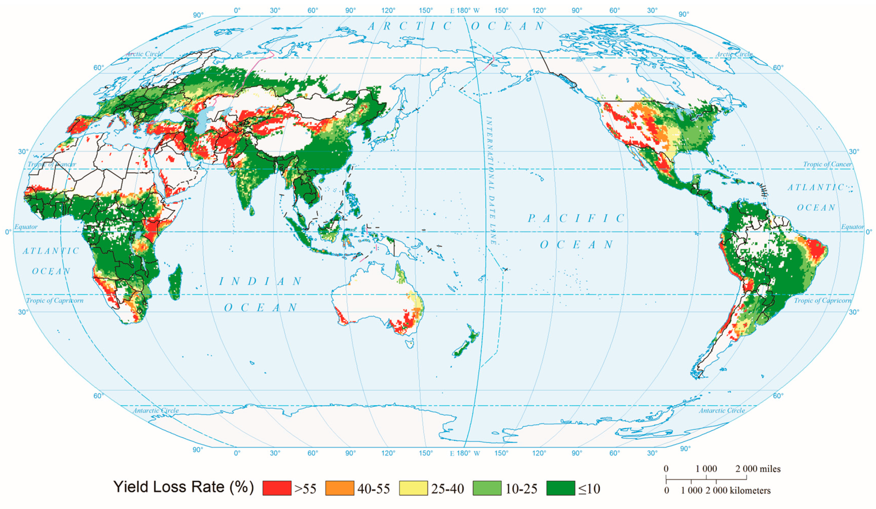
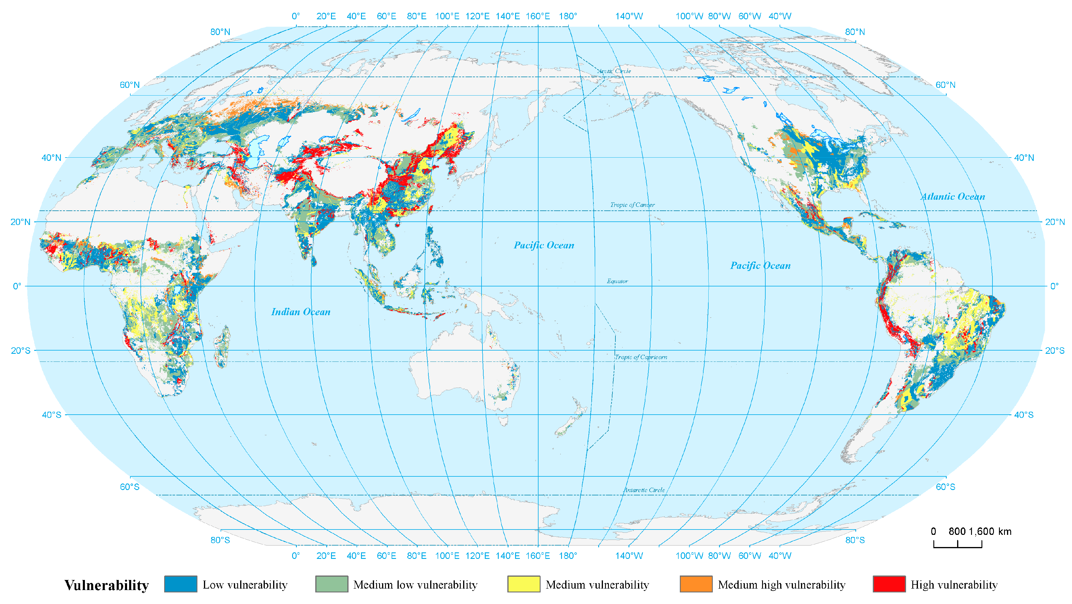
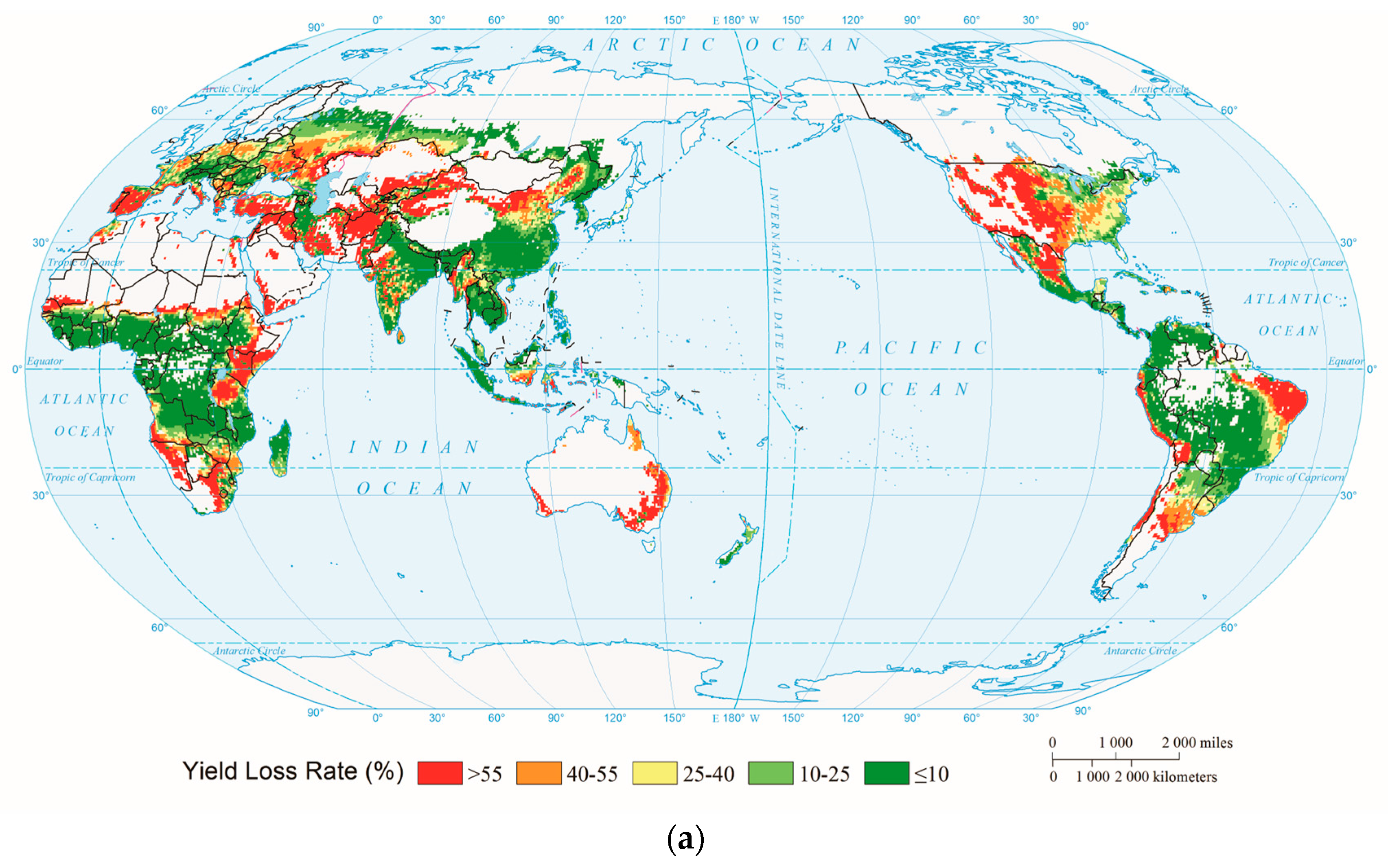
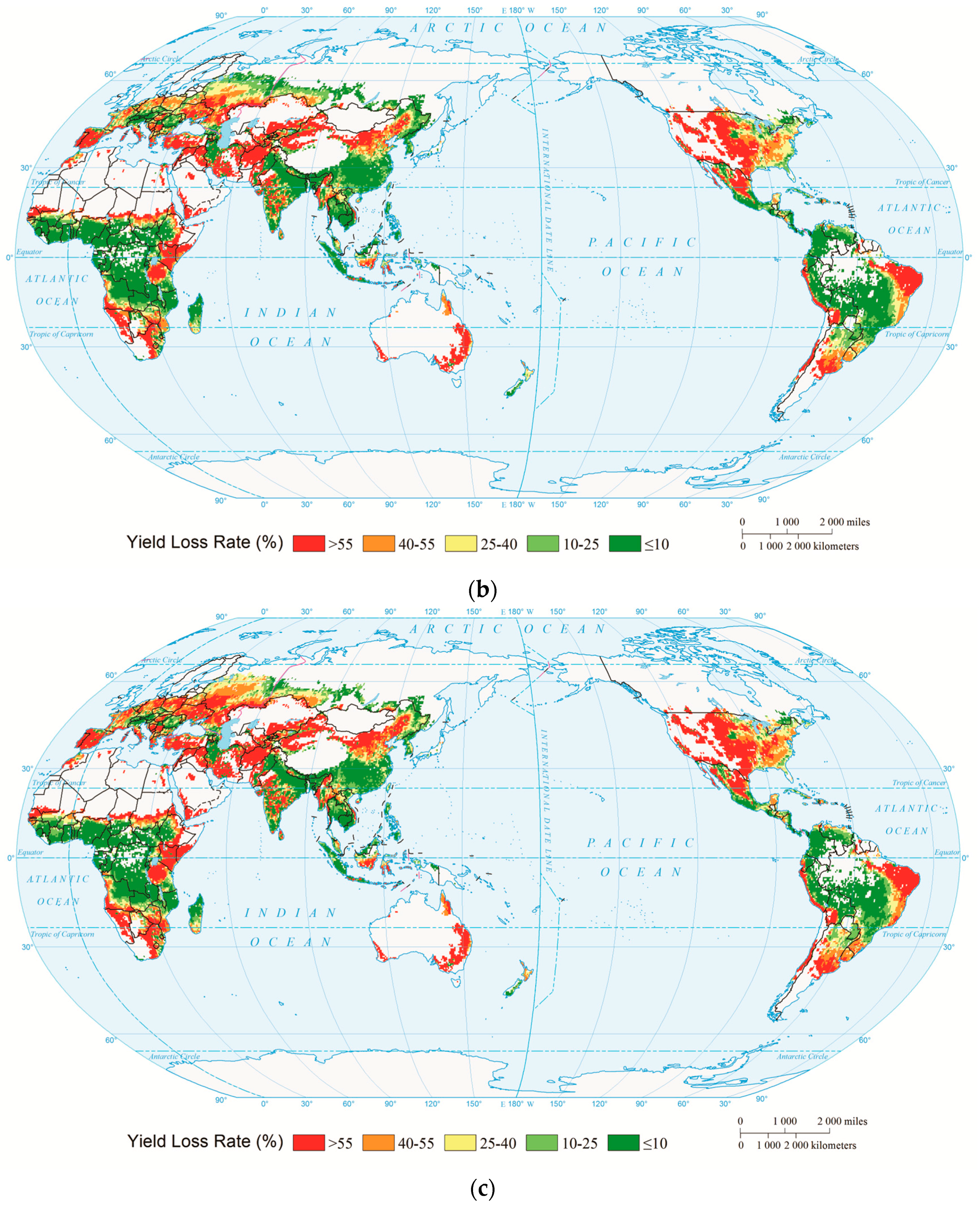
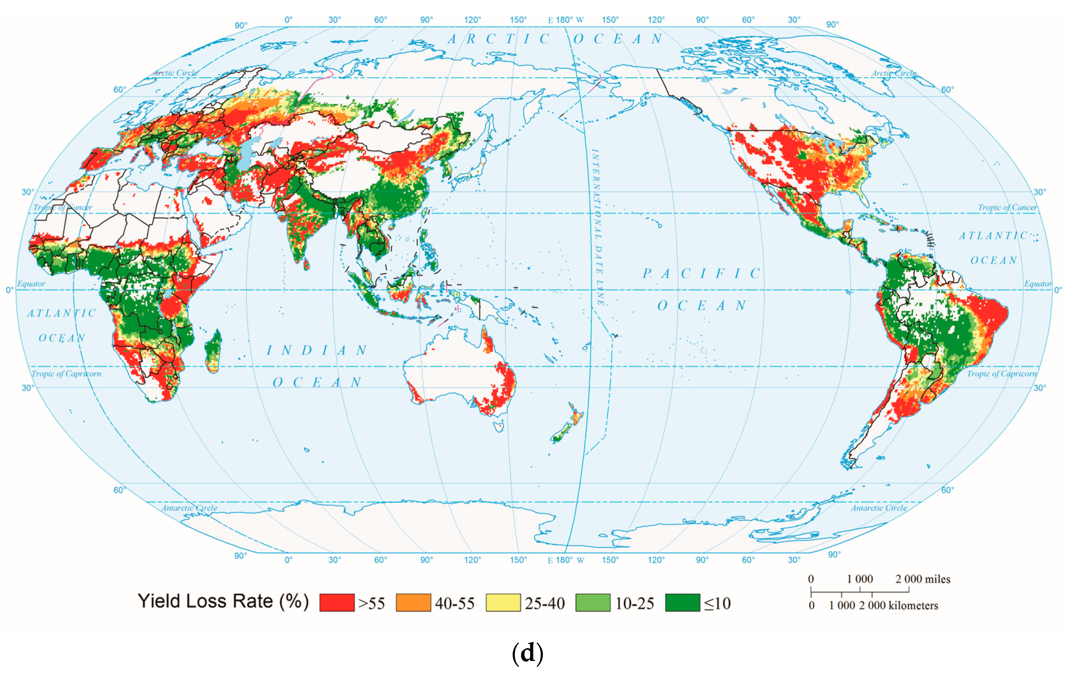
3.3. Maize Drought Risk on a Global Scale

According to information diffusion theory, the probability of different drought intensities was calculated in each grid cell based on 30-year historical data (Figure 8).
Global maize drought risk was calculated according to the optimal vulnerability surface (CFRAG), as shown in Figure 9.
The expected global yield loss rate for maize is 19.18%. The rate rises with increasing return period, reaching 29.18%, 32.76%, 36.89%, and 38.26% in a 10-year, 20-year, 50-year, and 100-year return period, respectively (Appendix B). Globally, areas with high maize drought risk (red zone) are located in mid-latitude regions (30°–50°), mainly including the Iberian Peninsula, the Midwestern United States, northwestern China, Central Asia, eastern Brazil, Chile, Spain, and certain low-latitude regions near the Equator, including East Africa and northeastern Brazil.
Based on Figure 9 (Table 3), the risk for all grid cells in each country was averaged. The results suggest that the average yield loss rate may exceed 50% when Chile, Afghanistan, Iraq, Spain, and certain other countries suffer from a drought disaster. The average yield loss rate of maize in the United States and Australia is about 30%–40%, whereas that in China and Brazil is less than 20%. The highest values among the countries in Table 3 are about 80%–90%. The differences in maize drought risk among countries are obvious. Some of these countries are major grain-producing countries, and food shortages may occur once they have suffered a severe loss in yield. Therefore, countries with higher maize drought risk should strengthen their predictive capabilities for drought disasters to minimize the economic losses caused by droughts.

4. Discussion

4.1. Relationship between CFRAG and Crops

In this research, the “L-D-E” vulnerability surface was best fitted with coarse fragment content (CFRAG) as the environmental indicator. With increasing CFRAG, LR of maize first decreased and then increased under the same hazard condition. A higher CFRAG is helpful for soil permeability because it makes it easier for water to reach plant roots and be absorbed. When CFRAG exceeds a threshold value, however, the water-holding capacity of the soil decreases, soil moisture is more likely to evaporate, and plants are more vulnerable to drought. Some CFRAG studies have proposed that CFRAG is negatively correlated with maize yields [59]. According to Grewal’s experiment with different levels of gravel content (18%, 28%, and 40%) as CFRAG, an increasing proportion of gravel led to decreasing soil nutrient content and soil water-holding capacity and a yield that showed a downward trend [60]. Driessen described the quantitative effect of CFRAG on a productivity index (decreasing from 100% to 0% with gravel contents of 10% to 70%), but the effect was due to the reduction of available plant water rather than rooting depth [61]. When CFRAG is higher than the threshold value, it will negatively affect soil moisture and nutrition, resulting in yield reduction and higher crop vulnerability.

4.2. Significance of Vulnerability Surfaces

In a similar study, researchers calculated the global drought risk for maize by fitting vulnerability curves for different areas [30]. However, two-dimensional vulnerability curves can only express the relationship between hazard intensity and yield loss, without considering the environmental dimension. Environmental differences can be embodied only by artificially dividing the study area into different units. The vulnerability surface is different from the vulnerability curve. Its significant advantage lies in its consideration of the differences in environmental elements. Therefore, different environmental elements correspond to different relationships between hazard intensity and yield loss rate, and errors in research results caused by artificial division into different environment zones are thus avoided. Another advantage of the vulnerability surface is that it can be incorporated into multi-scale studies. This means that the maize drought vulnerability surface calculated based on a 0.5° × 0.5° grid in this study can be converted into vulnerability assessment results at different scales according to the research resolution requirement or the resolution of relevant environmental indicators, which may even be higher than 0.5° × 0.5°.
For risk assessment studies based on the vulnerability curve, the vulnerability surface can be divided into a number of vulnerability curves according to different environmental indicators. The vulnerability surface can be considered as an infinite number of vulnerability curves. For risk assessment studies based on the vulnerability index, the vulnerability assessment can be completed using the integrals of the vulnerability curves. The larger the integral values, the more vulnerable crops are. As shown in Figure 10, vulnerability under different soil types was calculated and classified according to the maize “L-D-E” vulnerability surface (based on 0.5° × 0.5° data) and soil data (0.0833° × 0.0833°) curves, thus the vulnerability assessment resolution can be converted from lower (0.5° × 0.5°) to higher (0.0833° × 0.0833°).
Therefore, the vulnerability surface further considers differences in environmental elements, and can be converted to different scales due to its ability to express continuous changes in vulnerability. It has certain advantages for large-scale (such as global) vulnerability or risk assessment.

4.3. Validity of Risk Assessment Results Based on the Vulnerability Surface

The planting range data for maize come from the Center for Sustainability and the Global Environment (SAGE), University of Wisconsin-Madison [49]. These data were combined with national, state, and county statistical data that described the harvested area of 175 crops (spatial resolution: 0.0833° × 0.0833°). In this research, the spatial resolution was resampled to 0.5° × 0.5° to unify research resolution. The risk was assessed as long as maize was planted in the grid cell. Note that the planted proportion of each grid cell was not considered in the risk assessment. Indeed, gross production or planted proportion has little effect on yield loss rate in each grid cell. Therefore, this study, which used yield loss rate to represent risk, would be little influenced.
Cases of global maize drought risk assessment are rare. Some researchers have calculated precipitation, soil moisture, and other indicators for different months under various scenarios according to different climate models to assess future drought severity due to climate change [62,63]. The results show that the United States, the Amazon Basin, and Europe are future arid regions in different climate models. Other researchers have considered the Palmer Drought Severity Index (PDSI) and other drought-related indices on a global scale to evaluate the frequency [64], trend [65], and soil moisture and temperature changes [66] associated with future drought. Overall, most research results show that serious drought areas will be distributed mainly in central Asia, southwestern Europe, southern Africa, western and central North America, and northeastern South America. To test the validity of the results reported in this paper, those reported by Li [64] were chosen for comparison. A correlation analysis (Table 4) was completed between the pattern of maize drought risk reported in this paper (the sum of the expected loss rates for each continent) and Li’s results (DRI of baseline for each continent). The correlation coefficient was 0.717, which shows a significant relationship at the 0.05 level.
Therefore, the results of this study, which are based on the maize vulnerability surface, are close to the pattern of existing results at continental scale. However, the evaluation results may be different in regional areas as a result of different methods and data.

5. Conclusions

The influence of drought on agriculture is serious. Research on crop response to drought can provide significant information to reduce agricultural losses caused by drought and promote sustainable agricultural development. In this research, a 3D vulnerability surface was fitted, and the global maize drought risk was evaluated. It was concluded that the vulnerability surface incorporating variations in environmental factors can express the continuous functional relationship between “Hazard”, “Loss (Loss rate)”, and “Environment”. In addition, the vulnerability assessment results can be converted into different scales based on the vulnerability surface due to its ability to express continuous changes in vulnerability. Last but not least, the vulnerability surfaces can be used for quantitative drought risk assessment that directly denotes the probability of crop yield loss. The research provides a new method for research into biophysical vulnerability assessment.
In our previous studies, EPIC was used to simulate “Drought hazard-Crop yield loss” vulnerability curves to assess the drought risk of different crops (maize [67], wheat [68], and rice [69]). This study has proposed a new method for assessing vulnerability quantitatively and continuously by including the environment variable as an additional perspective on exposure. This method could be used for different crops, climate scenarios, and periods. It might constitute a promising direction for further research that could assess vulnerability comprehensively and quantitatively by studying the location change or adaption of different crop species.

Acknowledgments

This study was supported by the National Basic Research Program of China (973 Project): Relationship between Global Change and Environmental Risks and its Adaptation Paradigm (No. 2012CB955403) and the National Key Research and Development Program (No. 2016YFA0602402). This paper was improved by comments from Matthew Turner and A.-Xing Zhu from the University of Wisconsin-Madison. The valuable comments and suggestions from the editor and anonymous reviewers are also greatly appreciated.

Author Contributions

Hao Guo conceived the entire paper, analyzed the data, and wrote the paper; Xingming Zhang designed and performed the experiments and analyzed the data; Fang Lian and Yuan Gao polished the text of the paper; Degen Lin provided technical support; Jing’ai Wang polished the text and provided project support.

Conflicts of Interest

The authors declare no conflict of interest.

Appendix A

Similar to Figure 7, “L-D-E” vulnerability surfaces were fitted with other environmental indicators, as shown in Figure A1.
Figure A1. “L-D-E” vulnerability surfaces fitted with environmental indicators other than CFRAG: (a) elevation; (b) slope; (c) BULK; (d) TAWC; (e) SDTO; (f) CLPC; (g) TOTC; (h) PH.
Sustainability 08 00813 g011aSustainability 08 00813 g011b

Appendix B

Similar to Figure 9, global maize drought risk was mapped for different return periods, as shown in Figure B1.
Figure B1. Global maize drought risk for different return periods: (a) 10-year return period; (b) 20-year return period; (c) 50-year return period; (d) 100-year return period.
Sustainability 08 00813 g012aSustainability 08 00813 g012bSustainability 08 00813 g012c

References

  1. Stocker, T.F. Climate Change 2013: The Physical Science Basis; Working group I Contribution to the Fifth Assessment Report of the Intergovernmental Panel on Climate Change; Cambridge University Press: Cambridge, UK, 2014. [Google Scholar]
  2. Kelley, C.P.; Mohtadi, S.; Cane, M.A.; Seager, R.; Kushnir, Y. Climate change in the fertile crescent and implications of the recent syrian drought. Proc. Natl. Acad. Sci. USA 2015, 112, 3241–3246. [Google Scholar] [CrossRef] [PubMed]
  3. Allen, C.D.; Macalady, A.K.; Chenchouni, H.; Bachelet, D.; McDowell, N.; Vennetier, M.; Kitzberger, T.; Rigling, A.; Breshears, D.D.; Hogg, E.T. A global overview of drought and heat-induced tree mortality reveals emerging climate change risks for forests. For. Ecol. Manag. 2010, 259, 660–684. [Google Scholar] [CrossRef]
  4. Gleick, P.H. Water, drought, climate change, and conflict in syria. Weather Clim. Soc. 2014, 6, 331–340. [Google Scholar] [CrossRef]
  5. Charpentier, A. Insurability of climate risks. Geneva Pap. Risk Insurance Issues Pract. 2008, 33, 91–109. [Google Scholar] [CrossRef]
  6. Rosenzweig, C.; Elliott, J.; Deryng, D.; Ruane, A.C.; Müller, C.; Arneth, A.; Boote, K.J.; Folberth, C.; Glotter, M.; Khabarov, N. Assessing agricultural risks of climate change in the 21st century in a global gridded crop model intercomparison. Proc. Natl. Acad. Sci. USA 2014, 111, 3268–3273. [Google Scholar] [CrossRef] [PubMed]
  7. Pelling, M.; Maskrey, A.; Ruiz, P.; Hall, L.; Peduzzi, P.; Dao, Q.-H.; Mouton, F.; Herold, C.; Kluser, S. Reducing Disaster Risk: A Challenge for Development; United Nations Development Programme: New York, NY, USA, 2004. [Google Scholar]
  8. Palmer, W.C. Meteorological Drought; US Department of Commerce, Weather Bureau: Washington, DC, USA, 1965; Volume 30.
  9. McKee, T.B.; Doesken, N.J.; Kleist, J. The relationship of drought frequency and duration to time scales. In Proceedings of the 8th Conference on Applied Climatology, Anaheim, CA, USA, 17–22 January 1993; pp. 179–183.
  10. Dalezios, N.; Blanta, A.; Spyropoulos, N.; Tarquis, A. Risk identification of agricultural drought for sustainable agroecosystems. Nat. Hazards Earth Syst. Sci. 2014, 14, 2435–2448. [Google Scholar] [CrossRef]
  11. Woli, P.; Jones, J.; Ingram, K.; Paz, J. Forecasting drought using the agricultural reference index for drought (arid): A case study. Weather Forecast. 2013, 28, 427–443. [Google Scholar] [CrossRef]
  12. Chongfu, H. Principle of information diffusion. Fuzzy Sets Syst. 1997, 91, 69–90. [Google Scholar] [CrossRef]
  13. Dai, A. Characteristics and trends in various forms of the palmer drought severity index during 1900–2008. J. Geophys. Res. Atmos. 2011, 116. [Google Scholar] [CrossRef]
  14. Mpelasoka, F.; Hennessy, K.; Jones, R.; Bates, B. Comparison of suitable drought indices for climate change impacts assessment over australia towards resource management. Int. J. Climatol. 2008, 28, 1283–1292. [Google Scholar] [CrossRef]
  15. Conde, C.; Liverman, D.; Flores, M.; Ferrer, R.; Araújo, R.; Betancourt, E.; Villarreal, G.; Gay, C. Vulnerability of rainfed maize crops in Mexico to climate change. Clim. Res. 1998, 9, 17–23. [Google Scholar] [CrossRef]
  16. Pogson, M.; Hastings, A.; Smith, P. Sensitivity of crop model predictions to entire meteorological and soil input datasets highlights vulnerability to drought. Environ. Model. Softw. 2012, 29, 37–43. [Google Scholar] [CrossRef]
  17. Dilley, M. Natural Disaster Hotspots: A Global Risk Analysis; World Bank Publications: Washington, DC, USA, 2005; Volume 5. [Google Scholar]
  18. Antwi-Agyei, P.; Fraser, E.D.; Dougill, A.J.; Stringer, L.C.; Simelton, E. Mapping the vulnerability of crop production to drought in Ghana using rainfall, yield and socioeconomic data. Appl. Geogr. 2012, 32, 324–334. [Google Scholar] [CrossRef]
  19. Simelton, E.; Fraser, E.D.; Termansen, M.; Forster, P.M.; Dougill, A.J. Typologies of crop-drought vulnerability: An empirical analysis of the socio-economic factors that influence the sensitivity and resilience to drought of three major food crops in China (1961–2001). Environ. Sci. Policy 2009, 12, 438–452. [Google Scholar] [CrossRef]
  20. Wu, H.; Wilhite, D.A. An operational agricultural drought risk assessment model for Nebraska, USA. Nat. Hazards 2004, 33, 1–21. [Google Scholar] [CrossRef]
  21. Jayanthi, H.; Husak, G.J.; Funk, C.; Magadzire, T.; Chavula, A.; Verdin, J.P. Modeling rain-fed maize vulnerability to droughts using the standardized precipitation index from satellite estimated rainfall—Southern Malawi case study. Int. J. Disaster Risk Reduct. 2013, 4, 71–81. [Google Scholar] [CrossRef]
  22. Wang, Z.; He, F.; Fang, W.; Liao, Y. Assessment of physical vulnerability to agricultural drought in China. Nat. Hazards 2013, 67, 645–657. [Google Scholar] [CrossRef]
  23. Li, Y.; Sperry, J.S.; Shao, M. Hydraulic conductance and vulnerability to cavitation in corn (Zea mays L.) hybrids of differing drought resistance. Environ. Exp. Bot. 2009, 66, 341–346. [Google Scholar] [CrossRef]
  24. Ming, X.; Xu, W.; Li, Y.; Du, J.; Liu, B.; Shi, P. Quantitative multi-hazard risk assessment with vulnerability surface and hazard joint return period. Stoch. Environ. Res. Risk Assess. 2015, 29, 35–44. [Google Scholar] [CrossRef]
  25. Birkmann, J. Risk and vulnerability indicators at different scales: Applicability, usefulness and policy implications. Environ. Hazards 2007, 7, 20–31. [Google Scholar] [CrossRef]
  26. White, G.F. Choice of Adjustment to Floods; University of Chicago: Chicago, IL, USA, 1964; p. 150. [Google Scholar]
  27. Smith, D. Flood damage estimation—A review of urban stage-damage curves and loss functions. Water SA 1994, 20, 231–238. [Google Scholar]
  28. Jayanthi, H.; Husak, G.J.; Funk, C.; Magadzire, T.; Adoum, A.; Verdin, J.P. A probabilistic approach to assess agricultural drought risk to maize in Southern Africa and millet in Western Sahel using satellite estimated rainfall. Int. J. Disaster Risk Reduct. 2014, 10, 490–502. [Google Scholar] [CrossRef]
  29. Jia, H.; Wang, J.; Cao, C.; Pan, D.; Shi, P. Maize drought disaster risk assessment of china based on EPIC model. Int. J. Digit. Earth 2012, 5, 488–515. [Google Scholar] [CrossRef]
  30. Yin, Y.; Zhang, X.; Lin, D.; Yu, H.; Shi, P. GEPIC-VR model: A GIS-based tool for regional crop drought risk assessment. Agric. Water Manag. 2014, 144, 107–119. [Google Scholar] [CrossRef]
  31. Lee, K.H.; Rosowsky, D.V. Fragility analysis of woodframe buildings considering combined snow and earthquake loading. Struct. Saf. 2006, 28, 289–303. [Google Scholar] [CrossRef]
  32. Wang, Z.; Song, W.; Li, T. Combined fragility surface analysis of earthquake and scour hazards for bridge. In Proceedings of the 15th World Conference on Earthquake Engineering, Lisbon, Portugal, 28 September 2012; pp. 24–28.
  33. McCarthy, J.J. Climate Change 2001: Impacts, Adaptation, and Vulnerability; Contribution of Working Group II to the Third Assessment Report of the Intergovernmental Panel on Climate Change; Cambridge University Press: Cambridge, UK, 2001. [Google Scholar]
  34. Barros, V.; Field, C.; Dokke, D.; Mastrandrea, M.; Mach, K.; Bilir, T.; Chatterjee, M.; Ebi, K.; Estrada, Y.; Genova, R. Climate Change 2014: Impacts, Adaptation, and Vulnerability: Part B: Regional Aspects; Contribution of working Group II to the Fifth Assessment Report of the Intergovernmental Panel on Climate Change; Cambridge University Press: Cambridge, UK; New York, NY, USA, 2014. [Google Scholar]
  35. Challinor, A.; Wheeler, T.; Garforth, C.; Craufurd, P.; Kassam, A. Assessing the vulnerability of food crop systems in Africa to climate change. Clim. Chang. 2007, 83, 381–399. [Google Scholar] [CrossRef]
  36. Williams, J.; Jones, C.; Kiniry, J.; Spanel, D.A. The EPIC crop growth model. Trans. ASAE 1989, 32, 497–511. [Google Scholar] [CrossRef]
  37. Hempel, S.; Frieler, K.; Warszawski, L.; Schewe, J.; Piontek, F. A trend-preserving bias correction—The ISI-MIP approach. Earth Syst. Dyn. 2013, 4, 219–236. [Google Scholar] [CrossRef]
  38. United States Geological Survey (USGS). Available online: https://lta.cr.usgs.gov/GTOPO30 (accessed on 21 June 2013).
  39. International Institute for Applied Systems Analysis-Global Agro-Ecological Zones (GAEZ). Available online: http://www.gaez.iiasa.ac.at (accessed on 11 December 2012).
  40. International Soil Reference and Information Centre (ISRIC). Available online: http://www.isric.org/data/isric-wise-derived-soil-properties-5-5-arc-minutes-global-grid-version-12 (accessed on 14 October 2013).
  41. German Federal Ministry of Education and Research (BMBF): The ISIMIP Fast Track Project. Available online: https://www.isimip.org/outputdata (accessed on 14 October 2013).
  42. University of Wisconsin-Madison: Sustainability and the Global Environment (SAGE). Available online: http://nelson.wisc.edu/sage/data-and-models/datasets.php (accessed on 27 July 2014).
  43. University of Wisconsin-Madison Sustainability and the Global Environment (SAGE). Available online: http://nelson.wisc.edu/sage/data-and-models/crop-calendar-dataset/index.php (accessed on 29 June 2014).
  44. The University of Tokyo (OKI Laboratory). Available online: http://hydro.iis.u-tokyo.ac.jp/GW/result/global/annual/withdrawal/index.html (accessed on 19 June 2014).
  45. Land Use and the Global Environment (LUGE). Available online: http://www.ramankuttylab.com/data.html (accessed on 26 March 2014).
  46. Food and Agriculture Organization (FAO). Available online: http://faostat.fao.org (accessed on 26 March 2014).
  47. Fischer, G.; Nachtergaele, F.; Prieler, S.; Teixeira, E.; Tóth, G.; van Velthuizen, H.; Verelst, L.; Wiberg, D. Global Agro-Ecological Zones (Gaez v3. 0): Model Documentation; International Institute for Applied Systems Analysis (IIASA): Laxenburg, Austria, 2012; Austria and the Food and Agriculture Organization of the United Nations (FAO): Rome, Italy, 2012.
  48. Batjes, N. Isric-Wise Derived Soil Properties on a 5 by 5 Arc-Minutes Global Grid (ver. 1.2); ISRIC: Wageningen, The Netherlands, 2012. [Google Scholar]
  49. Monfreda, C.; Ramankutty, N.; Foley, J.A. Farming the planet: 2. Geographic distribution of crop areas, yields, physiological types, and net primary production in the year 2000. Glob. Biogeochem. Cycles 2008, 22. [Google Scholar] [CrossRef]
  50. Sacks, W.J.; Deryng, D.; Foley, J.A.; Ramankutty, N. Crop planting dates: An analysis of global patterns. Glob. Ecol. Biogeogr. 2010, 19, 607–620. [Google Scholar] [CrossRef]
  51. Tan, G.; Shibasaki, R. Global estimation of crop productivity and the impacts of global warming by GIS and EPIC integration. Ecol. Model. 2003, 168, 357–370. [Google Scholar] [CrossRef]
  52. Potter, P.; Ramankutty, N.; Bennett, E.M.; Donner, S.D. Characterizing the spatial patterns of global fertilizer application and manure production. Earth Interact. 2010, 14, 1–22. [Google Scholar] [CrossRef]
  53. De Barros, I.; Williams, J.R.; Gaiser, T. Modeling soil nutrient limitations to crop production in semiarid ne of Brazil with a modified EPIC version II: Field test of the model. Ecol. Model. 2005, 181, 567–580. [Google Scholar] [CrossRef]
  54. Gaiser, T.; de Barros, I.; Sereke, F.; Lange, F.-M. Validation and reliability of the EPIC model to simulate maize production in small-holder farming systems in tropical sub-humid West Africa and semi-arid Brazil. Agric. Ecosyst. Environ. 2010, 135, 318–327. [Google Scholar] [CrossRef]
  55. Wang, X.C.; Li, J. Evaluation of crop yield and soil water estimates using the EPIC model for the loess plateau of China. Math. Comput. Model. 2010, 51, 1390–1397. [Google Scholar] [CrossRef]
  56. Wang, X.C.; Li, J.; Tahir, M.N.; De Hao, M. Validation of the EPIC model using a long-term experimental data on the semi-arid loess plateau of China. Math. Comput. Model. 2011, 54, 976–986. [Google Scholar] [CrossRef]
  57. Huang, C.; Moraga, C. Extracting fuzzy if–then rules by using the information matrix technique. J. Comput. Syst. Sci. 2005, 70, 26–52. [Google Scholar] [CrossRef]
  58. Hao, L.; Zhang, X.; Liu, S. Risk assessment to China’s agricultural drought disaster in county unit. Nat. Hazards 2012, 61, 785–801. [Google Scholar] [CrossRef]
  59. Khakural, B.; Robert, P.; Mulla, D. Relating Corn/Soybean Yield to Variability in Soil and Landscape Characteristics. Available online: https://dl.sciencesocieties.org/publications/books/abstracts/acsesspublicati/precisionagricu3/117 (accessed on 15 August 2016).
  60. Grewal, S.; Singh, K.; Dyal, S. Soil profile gravel concentration and its effect on rainfed crop yields. Plant Soil 1984, 81, 75–83. [Google Scholar] [CrossRef]
  61. Leenaars, J.; Hengl, T.; González, M.R.; de Jesus, J.M.; Heuvelink, G.; Wolf, J.; van Bussel, L.; Claessens, L.; Yang, H.; Cassman, K. Root Zone Plant-Available Water Holding Capacity of the Sub-Saharan Africa Soil, Version 1.0. Gridded Functional Soil Information (Dataset RZ-PAWHC SSA v. 1.0); ISRIC Report; ISRIC: Wageningen, The Netherlands, 2015; Volume 2. [Google Scholar]
  62. Wang, G. Agricultural drought in a future climate: Results from 15 global climate models participating in the IPCC 4th assessment. Clim. Dyn. 2005, 25, 739–753. [Google Scholar] [CrossRef]
  63. Sheffield, J.; Wood, E.F. Projected changes in drought occurrence under future global warming from multi-model, multi-scenario, IPCC AR4 simulations. Clim. Dyn. 2008, 31, 79–105. [Google Scholar] [CrossRef]
  64. Li, Y.; Ye, W.; Wang, M.; Yan, X. Climate change and drought: A risk assessment of crop-yield impacts. Clim. Res. 2009, 39, 31–46. [Google Scholar] [CrossRef]
  65. Burke, E.J.; Brown, S.J.; Christidis, N. Modeling the recent evolution of global drought and projections for the twenty-first century with the hadley centre climate model. J. Hydrometeorol. 2006, 7, 1113–1125. [Google Scholar] [CrossRef]
  66. Dai, A. Increasing drought under global warming in observations and models. Nat. Clim. Chang. 2013, 3, 52–58. [Google Scholar] [CrossRef]
  67. Yin, Y.; Zhang, X.; Yu, H.; Lin, D.; Wu, Y. Mapping drought risk (maize) of the world. In World Atlas of Natural Disaster Risk; Springer: Berlin, Germany, 2015; pp. 211–226. [Google Scholar]
  68. Zhang, X.; Guo, H.; Yin, W.; Wang, R.; Li, J.; Yue, Y. Mapping drought risk (wheat) of the world. In World Atlas of Natural Disaster Risk; Springer: Berlin, Germany, 2015; pp. 227–242. [Google Scholar]
  69. Zhang, X.; Lin, D.; Guo, H.; Wu, Y. Mapping drought risk (rice) of the world. In World Atlas of Natural Disaster Risk; Springer: Berlin, Germany, 2015; pp. 243–258. [Google Scholar]
Figure 1. Overall study procedure.
Sustainability 08 00813 g001
Figure 2. Parameter adjustment (assuming the N-th cycle is the current one): Rule 1: the step length of the N-th adjustment = initial parameters × 0.2, and the direction is the same as the (N-1)-st adjustment (the default is positive if this is the first time). Rule 2: the step length of the N-th adjustment = [(parameter value of (N-1)-st adjustment) − (parameter value of (N-2)-nd adjustment)] × 0.5, and the direction is opposite to that of the (N-1)-st adjustment.
Sustainability 08 00813 g002
Figure 3. Generation of “L-D-E” samples in each grid cell.
Sustainability 08 00813 g003
Figure 4. Hazard assessment in each grid cell.
Sustainability 08 00813 g004
Figure 5. Flowchart of maize drought risk assessment.
Sustainability 08 00813 g005
Figure 6. Scatter plots of simulated and actual yield of global maize over four years: (a) 2001; (b) 2002; (c) 2003; (d) 2004.
Sustainability 08 00813 g006
Figure 7. “L-D-E” vulnerability surface with CFRAG as environmental indicator. (a,b) represent different perspectives; vulnerability surfaces with other environmental indicators are shown in Appendix A.
Sustainability 08 00813 g007
Figure 8. Global drought intensity for maize by different return periods: (a) 10-year return period; (b) 20-year return period; (c) 50-year return period; (d) 100-year return period. The darker areas have a higher probability of maize drought.
Sustainability 08 00813 g008aSustainability 08 00813 g008b
Figure 9. Global expected annual maize drought risk. Red areas have a higher risk of maize drought, indicating that droughts can lead to high yield loss rates of maize in these regions, whereas green areas have a lower risk, meaning that maize in these areas is less affected by droughts. This figure shows only the expected risk map; the return period maps are shown in Appendix B.
Sustainability 08 00813 g009
Figure 10. Vulnerability of global maize to drought (0.0833° × 0.0833°). The vulnerability assessment results were divided into five levels based on the method of natural breaks (jenks) in ArcGIS. The redder the area in the picture, the larger the integral of the corresponding vulnerability curve, and the higher the vulnerability. If the value is smaller, the vulnerability is lower.
Sustainability 08 00813 g010
Table 1. Study data.
Data CategoryNameSourceSpatial ResolutionTemporal Resolution
Geographical environmental dataDEMUnited States Geological Survey (USGS) [38]0.0833° × 0.0833°1996
SlopeInternational Institute for Applied Systems Analysis-Global Agro-Ecological Zones (GAEZ) [39]0.0833° × 0.0833°2002
SoilInternational Soil Reference and Information Centre (ISRIC) [40]0.0833° × 0.0833°2012
MeteorologicalGerman Federal Ministry of Education and Research (BMBF):The ISIMIP Fast Track project [41]0.5° × 0.5°1971–2099
Extent of maizeUniversity of Wisconsin-Madison: Sustainability and the Global Environment (SAGE) [42]0.0833° × 0.0833°2000
Field management dataGrowth period of maizeUniversity of Wisconsin-Madison Sustainability and the Global Environment (SAGE) [43]0.5° × 0.5°2010
IrrigationThe University of Tokyo (OKI Laboratory) [44]0.5° × 0.5°2010
FertilizerLand Use and the Global Environment (LUGE) [45]0.5° × 0.5°2011
Calibration dataActual yield of global maizeFood and Agriculture Organization (FAO) [46]National (regional) unit2000–2004
Table 2. Parameters of the drought vulnerability surface of maize.
IndicatorabcdefR2RMSE
Elevation384.010.353.391.09 × 10−71167.2399.120.993392.89636
Slope−90.220.353.393.91 × 10−5−164.3997.980.993382.89996
CFRAG−15.650.363.360.00710.9498.880.993422.89062
BULK0.440.293.520.41−13.752.620.955187.54344
TAWC9.710.293.520.0008−184.1864.820.956207.45699
SDTO100.320.353.40−0.0001826.5199.340.993382.89889
CLPC−421.920.363.37−0.00156.9199.800.993342.90779
TOTC103.860.353.38−0.00019171.47103.810.993422.89104
PH0.440.303.490.02−54.3921.870.955897.48403
Table 3. Expected value of maize yield loss rate in high-risk countries.
CountryMaximum Yield Loss Rate (%)Minimum Yield Loss Rate (%)Average Yield Loss Rate (%)
Afghanistan93.85067.63
Australia92.230.4548.00
Brazil83.32011.59
Chile1000.0664.64
China99.97019.75
Iraq99.487.9670.32
Spain98.91051.46
United States97.260.0330.52
Table 4. Comparison of results with those of Li’s research [64].
ContinentNormalized Value of Risk in This StudyNormalized Value of Risk in Li’s Study
North America10.30
Europe0.640.22
Africa0.961
South America0.640.37
Oceania0.150
Southern Asia0.070.25
South East Asia00.22
Eastern Asia0.560.29
Middle East0.800.43

