Article

Ecosystem Services and Ecological Restoration in the Northern Shaanxi Loess Plateau, China, in Relation to Climate Fluctuation and Investments in Natural Capital

1
State Key Laboratory of Earth Surface Processes and Resource Ecology, Faculty of Geographical Science, Beijing Normal University, Beijing 100875, China
2
College of Resources Science and Technology, Faculty of Geographical Science, Beijing Normal University, Beijing 100875, China
3
Department of Environmental Engineering, Chinese Academy for Environmental Planning, Beijing 100012, China
4
Fujian Academy of Agricultural Sciences, Fuzhou 350003, China
5
Institute of Geographic Sciences and Natural Resources Research, Chinese Academy of Sciences, Beijing 100101, China
6
Department of Science and Technology, Parthenope University of Naples, Centro Direzionale-Isola C4, 80143 Napoli, Italy
7
Joint Center for Global change and China Green Development, Beijing Normal University, Beijing 100875, China
*
Author to whom correspondence should be addressed.
Sustainability 2017, 9(2), 199; https://0-doi-org.brum.beds.ac.uk/10.3390/su9020199
Submission received: 7 December 2016 / Accepted: 19 January 2017 / Published: 1 February 2017
(This article belongs to the Section Environmental Sustainability and Applications)

Abstract

:
Accurately identifying the spatiotemporal variations and driving factors of ecosystem services (ES) in ecological restoration is important for ecosystem management and the sustainability of nature conservation strategies. As the Green for Grain project proceeds, food provision, water regulation and climate regulation services in the Northern Shaanxi Loess Plateau (NSLP) are changing and have caused broad attention. In this study, the dynamic pattern of the normalized differential vegetation index (NDVI) and the main drivers of grain production (GP), water yield (WY) and net primary production (NPP) in the NSLP from 2000–2013 are identified by incorporating multiple data and methods, in order to provide a better understanding of how and why ES change during ecological restoration. WY was simulated by hydrological modeling, and NPP was estimated with the Carnegie Ames Stanford Approach (CASA) model. The results show that vegetation restoration continued from 2000–2013, but fluctuated because of the comprehensive influence of climate and human activity. GP and NPP both exhibited significantly increasing trends, while changes in WY occurred in two stages: decline (2000–2006) and growth (2007–2013). Spatially, significantly increasing trends in NPP and WY were detected in 52.73% and 24.76% of the region, respectively, in areas that correspond with the Green for Grain project and high precipitation growth. Correlation and partial correlation analyses show that there were different dominant factors (i.e., natural vs. anthropogenic) driving ES change in the NSLP from 2000–2013. The change in WY was mainly driven by precipitation, while the improvements in GP and NPP can be attributed to investments in natural capital (i.e., chemical fertilizer, agricultural machinery power and afforestation). We also found that vegetation restoration can produce positive effects on NPP, but negative effects on WY by using response analyses of WY or NPP change to NDVI change, demonstrating that additional research on the role of water in vegetation restoration is needed. Our results provide support for ES management and the sustainable development of ecological restoration in the NSLP.

1. Introduction

China has been the world’s second largest economy by the pursuit of rapid economic development, but the costs of this success are reflected in high levels of ecological degradation [1]. In China, natural disasters (e.g., flood) caused by environmental degradation occur more frequently and have severely impacted sustainable socioeconomic development in recent decades [2]. The Chinese government has implemented a series of ecological projects for improving the eco-environment. For example, Green for Grain (GFG), launched in 1999, is the largest eco-environmental construction project and important nature conservation program in China. GFG involves the effort to return cultivated land on steep slopes to perennial vegetation and afforest barren hills and wasteland using a government payment scheme, which engages millions of rural households as core agents of project implementation [2,3]. The Northern Shaanxi Loess Plateau (NSLP) is the core region of GFG, and it is also an ecologically-vulnerable area sensitive to climatic change [4,5]. Vegetation coverage of the NSLP has gradually improved since the implementation of GFG [6,7,8]. This improvement in vegetation cover has realized huge ecological effects, including the potential in sequestrating greenhouse gases [9,10] or regulating climate, which is a hot issue in the background of climate change. However, because some regions of GFG (e.g., NSLP) belong to the semi-arid area, some research has raised concerns about the problems of food security and water scarcity caused by GFG [11,12]. Climate regulation, water supply (yield) and food provision are all ecosystem services (ES), which are defined as the benefits people derive from ecosystems [13]. As a new round of GFG projects begin, we need to evaluate the benefits and impacts of previous GFG projects, which have been of great significance to the sustainability of GFG. ES certainly will change under ecological restoration, and this fact has received significant attention in recent years [1,14,15,16]. ES can build a “bridge” between ecological systems and human social systems and can be used to evaluate the benefits and impacts of nature conservation strategies [17]. In recent years, the Ecosystem Services Partnership, the Intergovernmental Science Policy Platform on Biodiversity and Ecosystem Services (IBPES), ecoSERVICES (a core project of Future Earth investigating the impact of biodiversity change on ecosystem functioning and services, and human well-being) and the Group on Earth Observations Biodiversity Observation Network (GEO-BON) have been established. One objective of these scientific programs is to assess ES comprehensively and promote the management and application of ES [18], and this requires knowledge of their dynamic features and driving factors.
As co-productions of natural and human systems [19,20], ES are affected by both natural factors (e.g., climatic change) and anthropogenic factors. According to the Millennium Ecosystem Assessment, the impact of climatic change on ES is growing [13]. Because it influences ecosystem structure and function, climatic change can significantly alter the capacity of ecosystems to provide services [21,22], but the relationships between climatic change and various ES can be either positive or negative, and they require careful analysis [21,23,24]. Humans can change ES in direct ways (e.g., land cover change, overexploitation, pollution) and indirect ways (e.g., population growth, economic activity, technical progress) [25,26]. One of the most direct anthropogenic factors, land cover change, has been an important contributor to changes in ES over the past 50 years [13]. Extensive croplands have been converted into woodlands, and natural vegetation has been restored in the NSLP, which has had a dramatic impact on ES. Current research shows that ES significantly changed in the Loess Plateau after GFG [3,27,28]. However, the processes and main drivers of different ES changes during the whole GFG period in the NSLP still need to be further elucidated. Quantitative relationships between vegetation restoration and different ES are not yet fully understood.
Here, we focus on food provision, water regulation and climate regulation in the NSLP, which are all highly related to the GFG project and interact with each other. By incorporating multi-source data and statistical methods, we investigated the dynamic patterns of vegetation and the main drivers of different ES changes in the NSLP from 2000–2013. In particular, we: (i) assessed the processes and the trends in vegetation restoration using the normalized difference vegetation index (NDVI); (ii) assessed the processes and trends in the difference of ES changes and their responses to vegetation restoration; and (iii) quantified the relationships between natural or anthropogenic factors and ES and identified the main drivers of different ES changes.

2. Study Area

Located in northern Shaanxi Province, China (35°21′–39°34′ N and 107°41′–110°31′ E) (Figure 1b), the NSLP covers an area of approximately 8.03 × 10⁴ km2 and consists of 25 counties (Figure 1a) belonging to two prefectures, Yan’an and Yulin (Figure 1c). High in the west and becoming lower in the east, the NSLP is a hilly, gullied area of the Loess Plateau [29,30]. The Mu Us desert in the northwest of Yulin has a primarily psammophyte vegetation type. Huanglong Mountain and Ziwu Mountain in southern Yan’an are the main forest-covered areas in the NSLP, and vegetation coverage there is relatively high. The eastern section of the NSLP is flat, and land use categories there mainly consist of cropland and grassland. Crops are mainly corn, soybeans and wheat, and the grassland is dominated by Miscanthus grass and clover [29]. This area has a semi-arid continental monsoon climate [30] and is characterized by warm and rainy summers and cold and dry winters [31].
From the maps of land use in 2000 (Figure S1a) and 2010 (Figure S1b), croplands, forestlands and grasslands showed the main land use types in our site. From a 2000–2010 land use transition matrix for the NSLP (Table 1), it can be seen that 694 km2 and 556 km2 of croplands in 2000 have been replaced by woodlands (including scrublands) and grasslands, respectively, due to the GFG project. Woodland coverage increased by 10.13%, while cropland coverage decreased by 4.19% during the 11-year period. At the same time, the grasslands increased by only 0.13%, because many grasslands were converted into woodlands. Dramatic changes in land use in the NSLP caused a series of ecological effects [2,32,33].

3. Methods

3.1. Vegetation Restoration Quantification

Vegetation indices are developed for evaluating vegetative covers using spectral measurements in the applications of remote sensing. Over forty vegetation indices have been developed in order to enhance vegetation response and minimize the effects of soil brightness, soil moisture, shadow and environmental effects [35]. NDVI is the normalized difference vegetation index and calculated by reflectance in the near-infrared and red wavelengths [36,37]. The NDVI is sensitive to green leaf area and surface vegetation coverage [4,36] and has been widely used in ecological research [37,38,39]. A few research works [4,6,7,8,36,37,38,39] have demonstrated the potential of using NDVI to detect vegetation dynamics. After the GFG project was implemented for more than ten years, the low-yield slope croplands were transformed into grasslands and woodlands, and many barren hills and wastelands turned “green". High-resolution images of remote sensing can detect these changes. MODIS (Moderate Resolution Imaging Spectroradiometer) NDVI with a 250-m spatial resolution can be adapted for the higher resolution detection. To eliminate the influence of cloud cover and atmosphere, the annual maximum value of the NDVI was chosen for use in this study by the maximum value composites methods [40]. Through that, the continuity of NDVI time series was enhanced, and the temporal-spatial change of vegetation could be identified more accurately.

3.2. Ecosystem Services Quantification

According to the Millennium Ecosystem Assessment [13], more than twenty kinds of ES were listed and could be classified into provisioning services, regulating services, supporting services and cultural services. We only chose three typical and representative services, including food provision (provisioning service), hydrology regulation (regulating service) and climate regulation (regulating service) according to the availability of data, the feasibility of the method and the importance of ES. The explanation was as follows. Food provision service was directly related to human well-being. Moreover, food provision would be affected because of the reduction of cropland in our site. Hydrology regulation was a significant and key service because our site was located in a semi-arid area. Moreover, the increase of forest area might consume more water because of more intense transpiration. In our site, ecosystems were very sensitive to climate changes [4], so climate regulation also was an important service. Moreover, in recent years, carbon emission growth caused by human activities was 13.96% per year in this area [41], and the government undertook the huge responsibility of carbon emission reduction in our site.

3.2.1. Grain Production

Grain production (GP) was selected as a proxy for the capacity of the food provision services. Data on wheat, corn and rice production were obtained at the provincial level from the Bureaus of Statistics [42] in our site (Yulin and Yan’an).

3.2.2. Water Yield

Water yield (WY) was selected as a proxy for hydrology regulation services. In arid and semi-arid areas, water budgets mainly depend on precipitation (PPT) and evapotranspiration (ET) [43,44]. WY is the result of the balancing of PPT and ET [29] and can be calculated as:
W Y = P P T E T
PPT was derived from the National Climatic Bureau and interpolated with the kriging method [45]. ET datasets were obtained from MOD16 ET products and estimated using the improved ET algorithm [46].
The interpolated precipitation data and the ET data (MOD16A3) came from different sources. We reduced the uncertainty through the following ways. The interpolated PPT data were set as the same spatial and temporal resolutions as satellite-derived ET data. The PPT and ET layers had the same coordinated system, and the calculation was processed in ArcGIS software with a stable environment. A few extreme values in the results were removed, and they were replaced by adjacent values.

3.2.3. Net Primary Production

Net primary production (NPP) is the key driver of the terrestrial carbon cycling, balancing CO2 and O2 and regulating global temperature [33]. Feng et al. [3] have found that the increase of carbon sequestration was mainly contributed by enhanced NPP on the Loess Plateau during the period of GFG implementation. The increment of NPP would enhance climate regulation services [47] in the NSLP, which is sensitive to climate changes. In this research, NPP was selected as a proxy for climate regulation services. The Carnegie Ames Stanford Approach (CASA) was employed to estimate per-pixel NPP at monthly intervals. CASA is a typical model of light use efficiency [48], and it needs relatively few parameters. Moreover, some parameters do not require actual measurement and can be obtained from remote sensing data. The total formula estimating NPP with CASA can be represented as [49]:
N P P = S O L × F P A R × E max × T a × T b × W × 0.5
where SOL is the total solar radiation (MJ/m2), which can be calculated from Equations (4) and (5); FPAR is the fraction of photosynthetically-active radiation (PAR) absorbed by the vegetation canopy, calculated following Potter et al. [48]; Emax is the maximum light use efficiency of main vegetation types, which in this study was set mainly according to the simulation results of Zhu et al. [50] in China as follows: 0.389 g C/MJ for evergreen needle-leaf forest, 0.692 g C/MJ for deciduous broadleaf forest, 0.475 g C/MJ for mixed forest and closed shrubland, 0.485 g C/MJ for deciduous needle-leaf forest, 0.429 g C/MJ for open shrubland, 0.542 g C/MJ for grassland and cropland and 0.389 g C/MJ for others [49]; Ta and Tb reflect temperature (T) stress on plant photosynthesis, calculated following Potter et al. [48]; W reflects moisture stress on plant photosynthesis, calculated following Xiao et al. [51]; and the coefficient 0.5 indicates that fraction of solar radiation falling in the PAR waveband (0.4–0.7 μm) [52].
Solar radiation can be calculated with the Angstrom formula that relates solar radiation to extraterrestrial radiation and sunshine percentage [53]. The local intensity of extraterrestrial radiation is determined by the angle between the direction of the Sun’s rays and the normal to the surface of the atmosphere [53]. The key equations for the solar radiation calculation are as follows:
E S O L = 24 ( 60 ) π S c d r ( w s s i n α s i n β + c o s α c o s β s i n w s )
S O L = E S O L ( a s + b s n N )
where ESOL is the extraterrestrial radiation (MJ/m2); Sc is the solar constant (1360 W/m2 or 49.20 MJ/m2·h2); dr, ws and β are the inverse relative Earth-Sun distance, sunset hour angle and solar decimation, respectively, calculated following Allen et al. [53]; α is the latitude of the meteorological stations (rad); as and bs are regression constants and variable in different latitudes, which were set according to the simulation results of Wen [54] in north China as follows: 0.344 for as and 0.390 for bs; n is the actual duration of sunshine; N is daylight hours; and n/N is the relative sunshine duration.

3.3. Change Trends and Response Relationships Analysis

3.3.1 Change Trends

Linear regression analysis was used to simulate NDVI/WY/NPP change trends at the pixel level or over the whole regional level [4,55,56]. The equation is as follows:
S l o p e = ( t = 1 n t × P A t 1 n × ( t = 1 n t ) × ( t = 1 n P A t ) ) / ( t = 1 n t 2 1 n × ( t = 1 n t ) 2 )
where a positive or negative Slope indicates an increasing or decreasing trend for NDVI/WY/NPP; n is the number of years; and PAt is the corresponding NDVI/WY/NPP value. The F-test method was used to analyze the statistical significance of the NDVI/WY/NPP change.

3.3.2. Response Relationships

The linear regression analysis was also used to explore the response relationships of ES change to vegetation restoration at the pixel scale. This paper is mainly focused on the response of regulating services to vegetation restoration, which has not been fully understood in current research [25,26,27,28,57]. The responses of WY change and NPP change to NDVI change at the pixel level were calculated using linear regression analysis. An increased or decreased result indicates a positive or negative response.

3.4. Correlation and Partial Correlation Analysis

Correlation and partial correlation analysis were used to analyze the relationships between ES and different driving factors. Both natural and anthropogenic factors have an important impact on ES [13]. In this paper, the climate fluctuations were chosen to be the main natural driving factors. The anthropogenic driving factors in our site were different for provisioning service (GP) and regulating services (WY and NPP). Temperature (T), precipitation (PPT), agricultural machinery power consumption, chemical fertilizer consumption and labor force input were chosen to be the driving factors of GP change, which was based on the study of Zhang et al. [58]. T, PPT and cumulative afforested area were chosen to be the driving factors of WY and NPP change, which agreed with the research of Xie et al. [59]. The cumulative afforested area could be understood as an indicator of GFG policy.
Partial correlation analysis is used when the two variables are related to the other variables at the same time; it will exclude the impact of the other variables and only analyze the correlation of the two variables [4,60]. For example, if there are three variables, the equation is as follows:
R x y - z = ( R x y R x z R y z ) / ( 1 R x z 2 ) ( 1 R y z 2 )
where Rxy-z is the partial correlation coefficient between x and y excluding the impact of z; Rxy is the correlation coefficient between x and y; Rxz is the correlation coefficient between x and z; Ryz is the correlation coefficient between y and z. The calculation of the correlation coefficient Rxy (or Rxz or Rxz) is detailed in Xu [60].

3.5. Data Preparation

Meteorological data from 32 weather stations (Table S1) within and near the NSLP were collected from the National Climatic Bureau [61], including monthly T, monthly PPT and sunshine duration during the study period.
The tile numbers of the remote sensing data in the NSLP were h26v05 and h27v05. A series of Moderate Resolution Imaging Spectroradiometer (MODIS) data for the CASA model during the 14-year period was derived from the MODIS on NASA’s Terra satellite [62], including surface albedo (MOD09A1), vegetation index (MOD13A2) and land cover type (MCD12Q1). The annual ET product (MOD16A3) was used to estimate WY, and the annual NPP product (MOD17A3) was used for comparison with the simulated NPP results of the CASA model. MOD16A3 and MOD17A3 were derived from the Numerical Terradynamic Simulation Group [63].
Data on agricultural machinery power consumption, chemical fertilizer consumption, labor force input in GP and cumulative afforested area during the 14-year period were obtained from provincial-level Bureaus of Statistics [42] in the NSLP and used for quantifying the relationships between ES and different driving factors.

4. Results

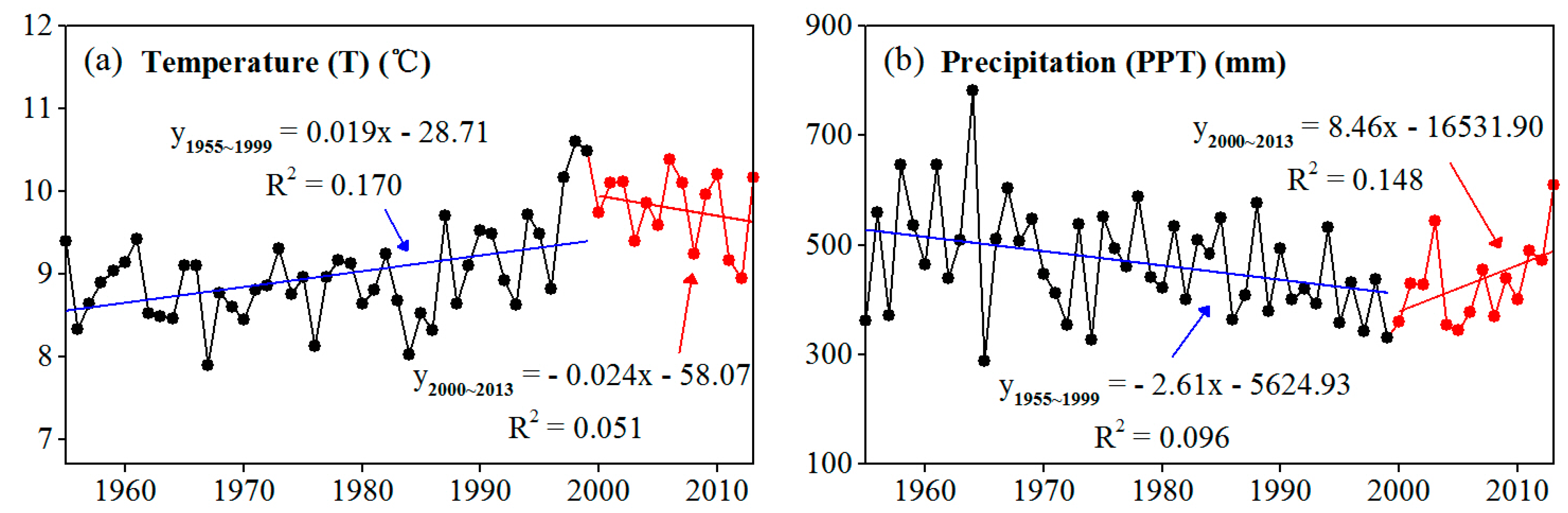
4.1. Climate Change Background

According to the original meteorological station data within our site, the area exhibited a warming and drying trend during the period from 1955–2013. We divided the complete interval into two periods, 1955–1999 and 2000–2013. From 1955–1999, we found that the annual mean T was 8.97 °C with an increase of 0.019 °C/year, and the annual mean PPT was 469.84 mm with a decrease of 2.61 mm/year (Figure 2). From 2000–2013, the annual mean T was 9.78 °C with a decrease of 0.024 °C/year, and the annual mean PPT was 433.48 mm with an increase of 8.46 mm/year (Figure 2). The annual mean T was higher and PPT lower from 2000–2013, while the changes of T and PPT were opposite to those of 1955–1999. At the pixel level, T and PPT both had higher values in the south than the north (Figure S2). In the last 14-year period, the T of 59.32% of the area was decreasing, while the PPT of the whole area was increasing (Figure S2). The global surface T was increasing over the past few decades, while the situation seemed to be different in our site. GFG policy might play a part of the role, because the most T decreasing regions were distributed in the GFG regions (Figure S2).

4.2. Vegetation Change

From 2000–2013, the NDVI exhibited a significantly increasing trend of 0.01/year (R2 = 0.858, p < 0.05), and thus, it improved 33.02% from 2000–2013 (Figure 3). From 2000–2002, the NDVI was in a period of rapid growth with an increase of 0.02/year, because the scale of GFG was larger in the early days of the project [4]. From 2003–2007, the NDVI was in a fluctuating period and kept decreasing from 2005–2007. Some vegetation (e.g., Hippophae rhamnoides L.) was planted, but it was not suitable for the semi-arid climate in the NSLP and needed more water when growing [64]. When PPT was low, these plants started to wither. More suitable vegetation was subsequently planted (e.g., Pinus sylvestris), and the NDVI started increasing from 2008.
In spatial terms, the NDVI in 85.62% of the area showed an increase (Figure 4b), and the NDVI in 52.96% of the area showed a significantly increasing trend (p < 0.05) (Figure 4c). Those areas were in the mid-eastern NSLP, which originally had low vegetation coverage (Figure 4a) and was therefore heavily involved in the GFG program from 2000–2013. At the same time, the NDVI in 14.38% of the area showed a slight decrease (Figure 4b), and these decreases were mostly not significant. The decreased areas were located in the southern NSLP (i.e., Ziwu Mountain and Huanglong Mountain) with high forest coverage. Some other researchers have found similar results either on larger scales [4,6] or at the same scale [64,65].

4.3. ES Change

4.3.1. GP Change

During 2000–2013, GP increased by 1.63-times and showed a significantly increasing trend of 24.87 t/km2·year (R2 = 0.824, p < 0.01) (Figure 5a). The croplands area decreased because of the GFG program, so the gross productivity increased only 1.3-times and showed a growth of 16.84 × 10⁴ t/year (Figure 5a). In 2005 and 2006, GP decreased (Figure 5a) because of drought stress (Figure 2b). A significant improvement in GP and gross productivity also was detected by other researchers [2,66,67].

4.3.2. WY Change

Total WY changed substantially during the 14-year period, ranging from 1723.61 m3/year in 2004 to 20,896.08 m3/year in 2013. The changes in WY can be divided into two stages: decline (2000–2006) and growth (2007–2013) (Figure 5b). Overall, WY in our site showed only a slight increase from 2000–2013, which was consistent with the PPT (Figure 2b). Other research [2] showed WY decreased after GFG in the whole Loess Plateau from 2000–2008. The results in this study show that WY decreased 24.81 mm during the same period.
Substantial regional variation in WY was detected under the influence of climate and vegetation coverage (Figure 6a). From the spatial change patterns, we see that 90% of the area experienced an increase in WY (Figure 6b). A decrease in WY was identified in the northwest NSLP, including Dingbian County, Jingbian County and Wuqi County. The annual growth rate of PPT was low in those areas. The change in 75.24% of the area was not significant, and 24.76% of the area experienced significant growth (p < 0.05), as seen in northern Yulin, including Shenmu County and Fugu County (Figure 6c), where there was a high annual growth rate of PPT (>8 mm/year) (Figure S2).

4.3.3. NPP Change

NPP in our site ranged from 17.24 Tg (1012 g) C/year (214.72 g C/m2·year) in 2000 to 25.30 Tg C/year (315.09 g C/m2·year) in 2012. The changes in NPP can be divided into three stages: significant growth (2000–2002), decline (2003–2007) and fluctuation (2008–2013) (Figure 5c). The decline in NPP may be attributed to the death of vegetation, as we have previously described [64]. Overall, NPP in our site showed a significant increasing trend during the 14-year period (R2 = 0.542, p < 0.01), which indicated that NPP in local ecosystems had improved.
NPP showed a similar spatial pattern to the NDVI (Figure 4a,b and Figure 6d,e). An increase was observed in 88.79% of the area, principally the mid-eastern NSLP that had undergone ecological restoration through the GFG program. NPP in Ziwu Mountain and Huanglong Mountain areas had a decrease, and this may be attributed to environmental factors and natural succession [68]. The higher significance level indicates a more credible NPP variation trend. The increasing NPP trend was significant in 52.73% of the area, while the decreasing NPP was generally not significant (Figure 6f).

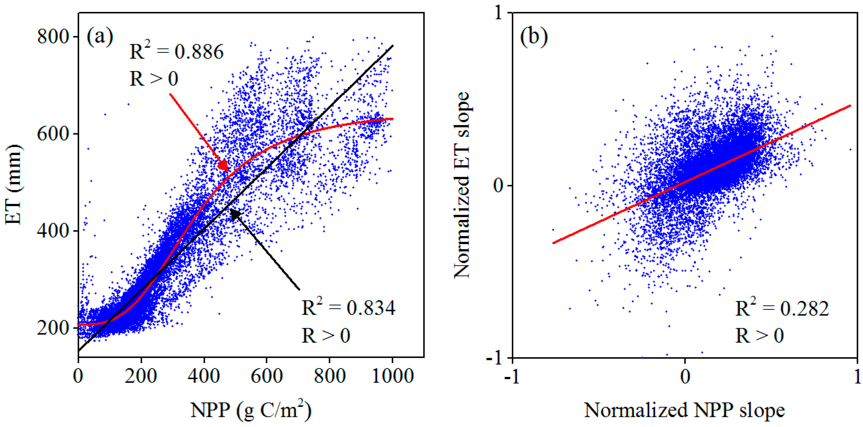
4.4. Response of ES Change to Vegetation Change

Response of regulating services to vegetation change is an important topic with the GFG project proceeding, but it has not been fully understood in current research [25,26,27,28,57]. At the pixel scale in our site, response relationships between regulating services (WY and NPP) and NDVI were analyzed and identified for the period from 2000–2013 (Figure 7). The response of WY change to NDVI change was negative (Figure 7a) (R2 = 0.012, R = −0.111, p < 0.01), which showed a negative relationship between WY and vegetation restoration. Vegetation restoration may have increased evapotranspiration (ET) and reduced regional WY, as has been found by other researchers [12,69,70]. The response of NPP change to NDVI change was positive (Figure 7b), which showed a positive relationship between NPP and vegetation restoration and that was consistent with previous research [2,59,68]. Moreover, Figure 7 showed that the response levels of regulating services to vegetation change were NPP > WY.

4.5. Relationships between ES and Different Driving Factors

From the results of correlation coefficients and partial correlation coefficients, both chemical fertilizer and agricultural machinery power were significant positive with GP from 2000–2013 in our site (Table 2). The GP correlation level of chemical fertilizer was higher than that of agricultural machinery power. The correlation between natural factors (T and PPT) and GP both were not significant (Table 2). A negative correlation was identified between labor force and GP from 2000–2013. During the study period, the labor force input in GP kept decreasing. However, other investments in GP including chemical fertilizer and agricultural machinery power were increasing, so the GP still kept increasing in our site. We divided the whole period into two stages: a GFG-extensive period (2000–2006) and a GFG-weakened period (2007–2013). It seemed that the correlation between different factors (natural or anthropogenic factors) and GP was stronger in the GFG-weakened period than in the GFG-extensive period (Table 2).
Over the whole regional scale, neither T nor cumulative afforested area were significantly correlated with WY from 2000–2013, but a significant positive correlation was identified between WY and PPT (Table 3). The strong response of WY change to PPT change at the pixel scale also showed that WY was significantly correlated with PPT (Figure 8a). The correlation between natural factors and WY was stronger in the GFG-weakened period than in the GFG-extensive period (Table 3). Through the correlation coefficients between WY and cumulative afforested area in different periods, it seemed that we could not judge that WY was increased or decreased with the increasing of cumulative afforested area. However, the partial coefficients in different periods were consistent and indicated that WY was decreased with the increasing of cumulative afforested area.
Over the whole regional scale, neither T nor PPT were significantly correlated with NPP (Table 4). NPP was decreased with the increasing in T, and the response of NPP change to T change at the pixel scale could indicate that (Figure 8b). The NSLP is a semi-arid area, so higher T would intensify soil evaporation and restrain plant photosynthesis [4]. The response of NPP change to T change at the pixel scale indicated that NPP was increased with the increasing in PPT (Figure 8c). Vegetation growth was restrained by moisture in the NSLP, so higher PPT enhanced plant activity and vegetation growth. During the 14-year period, the correlation between NPP and cumulative afforested area was significant and positive (Table 4). A stronger correlation was identified between NPP and cumulative afforested area during the GFG-extensive period than the GFG-weakened period (Table 4).

5. Discussion

5.1. Credibility of the Results

NPP and ET are crucial to the process of assessing ES change. NPP was estimated by the CASA model using multi-source data. ET was derived from the MODIS product with strong variability and it was a key and uncertain parameter in simulating WY. NPP and ET are affected by vegetation physiological factors and complex environment factors, so it is necessary to evaluate the credibility of the NPP and ET values.
The several simulated NPP values in the Loess Plateau have differences, and the main factors responsible include the simulation method, the study period and the scope of the Loess Plateau (Table 5) [71]. With respect to the scope of the Loess Plateau, annual NPP values simulated by Biome-BGC (Biogeochemical Cycles) were 10.08% lower for our site than for the whole area of the Loess Plateau. The simulated NPP value from the CASA model was lower by 11.69%–12.26% for our site than for the whole area of the Loess Plateau. This comparison showed that the CASA model used for our site performed well. Overall, the NPP values simulated by Biome-BGC were lower than the CASA values, partly because CASA simulates NPP at monthly intervals, and its estimates of the fraction of photosynthetic active radiation may therefore be larger [59].
The average NPP estimated by the CASA model (272 g C/m2·year) was higher than the MOD17-NPP (214 g C/m2·year) (Table 5). In the 25 counties of our site, simulated NPP values ranged from 141 g C/m2·year–695 g C/m2·year, and MOD17-NPP values ranged from 148 g C/m2·year–357 g C/m2·year. The correlation between simulated NPP and MOD17-NPP is significant in all 25 counties (Figure S3a). However, the simulated NPP was much higher than the MOD17-NPP in Fu County, Yichuan County, and especially in Huanglong County and Huangling County (Figure 9 and Figure S3). The above four counties are primarily located near Ziwu Mountain and Huanglong Mountain, which have high vegetation coverage (Figure 4a), so the NPP value should be higher there than in other counties, and some research corroborates this [3,68]. MOD17-NPP values were in middle range in the four counties, which shows that NPP simulated by the CASA model is more reasonable in those areas. Figure 9 shows that MOD17-NPP had small fluctuations in the 25 counties, which was mainly due to the simulation of MOD17-NPP at a global scale, while the NPP as estimated by CASA exhibited reasonable variation. During the 14-year period over the whole area, the annual simulated NPP and MOD17-NPP also had a significant correlation (R2 = 0.61, p < 0.01) (Figure S3b). Overall, the NPP simulated by CASA in this study is reliable.
In order to demonstrate the reliability of the ET dataset in our site, we offer the following points. First, the validity of MOD16-ET has been verified on different scales, as has been shown for Asia [73], Korea [74], China [75], Shaanxi Provence [76] and the Wei River Basin [77]. Second, the synergy between NPP and ET, which has been found in our site by Jia et al. [33], means that ET can be enhanced with the increases in NPP. At the pixel scale, the correlation between annual NPP and ET from 2000–2013 was analyzed and found to be significantly positive (R2 > 0.8, p < 0.01) (Figure 10a). The response of the ET change trend to the NPP change trend was also analyzed, and it too was significantly positive (R2 = 0.282, p < 0.01) (Figure 10b). As a result of this positive correlation between NPP and ET, the reliability of MOD16-ET in the NSLP is further enhanced.

5.2. Main Drivers of ES Changes

According to the relationships between GP and different factors (Table 2), neither T nor PPT were significantly correlated with GP during the study period, but the correlations between GP and the investments in agriculture (i.e., chemical fertilizer and agricultural machinery power) were significant (Table 2). Fu et al. [78] considered GP to be closely related to agricultural production conditions, artificial inputs and technical progress in the Loess Plateau. Our study showed that the increasing GP was mainly driven by the increasing agricultural investments in our site. Chemical fertilizer investment ranged from 155.71 kg/ha in 2000 to 330.29 kg/ha in 2013 (Figure 11a); it thus grew 1.12-times from 2000–2013 with a significantly increasing trend of 15.39 kg/ha·year (R2 = 0.928, p < 0.01). Agricultural machinery power grew 2.07-times and ranged from 19.80 kW/ha in 2000 to 60.77 kW/ha in 2013, with a significantly increasing trend (R2 = 0.996, p < 0.01) (Figure 11b). Moreover, our study also showed that chemical fertilizer input was more effective than agricultural machinery power input (Table 2). Other minor drivers of GP improvement in our site may include farm management and the construction of high quality basic croplands [2,65,66].
According to the relationships between WY and different factors (Table 3), both T and cumulative afforested area had a weak connection with WY change from 2000–2013 (Table 3). However, the negative effect of afforestation was significant in the GFG-extensive period (Table 3). The response of WY change to NDVI change showed there was a negative relationship between vegetation restoration and WY (Figure 7a). In this study, WY was calculated by subtracting ET from PPT. During the study period, ET increased with the growth of woodlands (Figure 11c), which can partly explain the negative relationship between afforestation or vegetation restoration and WY. However, the increase in ET was slight, and the annual growth in PPT (8.46 mm/year) was much larger than the growth in ET (1.90 mm/year), which suggests that the slight improvement of WY was mainly driven by PPT during the study period. The strong and positive response of WY change to PPT change (Figure 8a), significant correlation (Table 3) and linear fitting (Figure 12a) between WY and PPT can enhance the credibility of that conclusion. However, the afforestation producing the negative effect on WY still cannot be ignored.
According the relationships between NPP and different factors (Table 4), neither T nor PPT were significantly correlated with NPP during the study period, but the correlation between NPP and cumulative afforested area was significant. Xie et al. [59] consider land use change caused by GFG to be the main factor in increasing NPP in the Loess Plateau. Driven by GFG policy (the input of labor and funding), the decreasing croplands and increasing woodlands (including scrublands) were the main types of land use change in our site between 2000 and 2013. That change brought about the recovery of natural vegetation systems, which played a major role in the increase in NPP. Additionally, NPP was in fact significantly increasing in the mid-eastern NSLP, including Jia County, Hengshan County, Mizhi County, Wubao County, Zizhou County, Suide County, Zichang County, Qingjian County, Yanchuan County and Yan’an County, which correspond with the main GFG regions. The significant correlation (Table 4) and linear fitting (Figure 12b) between NPP and cumulative afforested area showed that the sustained growth of NPP was mainly caused by afforestation (or GFG policy).
The drivers involved in ES changes in our site from 2000–2013 are complex. For different ES, there are different dominant factors, some of them natural and other anthropogenic. The change in WY is attributed to the PPT belonging to the climate factor. The improvement in GP can be explained by the increasing in chemical fertilizer and agricultural machinery power, and the increasing in NPP can be explained by afforestation. Actually, these drivers (i.e., chemical fertilizer, agricultural machinery power and afforestation) can be attributed to the investments in natural capital. Ecosystems (e.g., forest ecosystem, farmland ecosystem) have been seen as natural capital assets, with the potential to generate a stream of vital life-support services [79]. The stable and persistent investments in natural capital are crucial to improve some ES. Recent research at a large scale [1] have found that the investments in natural capital starting in 2000 have significantly improved the key ES in China. On a relatively small scale, our analysis showed that the investments in the farmland system improved food provision and that the afforestation increased climate regulation service.

5.3. Sustainability of Ecological Restoration and ES

GFG policies increased GP and NPP in the NSLP, and those policies provide a natural foundation for maintaining ES. However, the ecosystem and socioeconomic system are interactive, and during this interaction, farmers’ attitudes and strategies are key to sustainable developments in ecological restoration [80]. Close cooperation between government and local stakeholders can maximize the effects of GFG projects [2]. The benefits produced by ecological restoration happen on a large scale (e.g., regional and national), while the costs of ecological restoration are undertaken by the local farmers. When the incomes of local farmers are temporarily reduced by ecological restoration projects, they typically re-plant later in the restored regions [81]. The conflicts caused by the differing scales of the costs and benefits have an impact on the sustainability of ecological restoration. After a dozen years of GFG in the NSLP, ecological restoration has shifted focus from ecological benefit to reconciling ecological and social benefits. However, according to the data derived from the National Poverty Alleviation Office in 2015, 44% of the counties in the GFG region are still poverty-stricken (i.e., Qingjian County, Zizhou County, Suide County, Mizhi County, Jia County, Wubao County, Hengshan County, Zichang County, Ansai County and Wuqi County). Achieving a win-win situation involving both ES and poverty alleviation is the primary objective for the sustainable development of ecological restoration.
Ecological restoration improves regulating services, but it may at the same time cause a drop in provision services and, thus, have a negative impact on local farmers. A few studies have found that there is a trade-off between provision services and regulating services [82,83,84]. However, our case study in the NSLP shows that the GP does not decrease, which mainly benefiting from sustaining investments in agriculture. This suggests that configuring effective compensation mechanisms (e.g., technological and economic) would contribute to the coordinated growth of both provision services and regulating services. Moreover, following the laws of ecological succession by choosing native tree species and developing more ecologically-informed GFG programs are both conducive to achieving stable and sustainable ecological restoration.

6. Conclusions

As a link between ecosystems and human well-being, ES are receiving more and more attention. As the GFG project proceeds, food provision, water regulation and climate regulation services in the NSLP are changing and have raised broad attention. To better understand the change trends and driving factors of the ES in the NSLP from 2000–2013, this study quantified the changes in NDVI/GP/WY/NPP and analyzed the relationships between GP/WY/NPP and different factors during the study period. The study found that, from 2000–2013, vegetation restoration was ongoing, but with fluctuation under the comprehensive influence of climate and human activity. GP and NPP both had a significantly increasing trend during the study period at the whole region scale in our site. Spatially, the regions with significant NPP growth corresponded strongly to the GFG counties. The changes in WY occurred in two stages: decline (2000–2006) and growth (2007–2013). There were different dominant factors (i.e., natural factors vs. anthropogenic factors) driving GP/WY/NPP change in our site from 2000–2013. The changes in WY were influenced mainly by PPT. The improvement in GP and NPP can be attributed to investments in natural capital (i.e., chemical fertilizer, agricultural machinery power and afforestation). Meanwhile, we also found that vegetation restoration produced positive effects on NPP, but negative effects on WY. According to our research, we offer the following recommendations to other landscapes experiencing similar policies. In the process of vegetation restoration, we should follow the laws of ecological succession and choose native tree species to avoid climate inadaptation. Configuring effective compensation mechanisms (e.g., technological and economic) in the nature conservation programs could relieve the losses of local people and would be conducive to achieving stable and sustainable ecological restoration.

Supplementary Materials

The following are available online at www.mdpi.com/2071-1050/9/2/199/s1, Figure S1: The land use types in the NSLP in 2000 (a) and 2010 (b), Figure S2: Spatial distribution and change trends in temperature and precipitation from 2000 to 2013 in the NSLP, Figure S3: Comparisons of simulated NPP and MOD17-NPP values in our site using (a) the average annual value from the 25 counties, and (b) the annual value from the 14-year period as a whole, Table S1: Information of weather stations within and near the Northern Shaanxi Loess Plateau (NSLP).

Acknowledgments

The authors gratefully acknowledge the financial support by the National Natural Science Foundation of China (41271549, 41671531), the Key Project of the National Societal Science Foundation of China (15ZDB163), the Fundamental Research Funds for the Central Universities (2014KJJCB33) and the China S&T Supporting Project (2012BAD14B03).

Author Contributions

Hejie Wei and Xiaobin Dong designed the paper. Hejie Wei collected the data and wrote the paper. Xiaobin Dong revised the paper. Kaixiong Xing contributed to the modification. Others were advisors. All authors have read and approved the final manuscript.

Conflicts of Interest

The authors declare no conflict of interest.

References

  1. Ouyang, Z.; Zheng, H.; Xiao, Y.; Polasky, S.; Liu, J.; Xu, W.; Wang, Q.; Zhang, L.; Xiao, Y.; Rao, E.; et al. Improvements in ecosystem services from investments in natural capital. Science 2016, 352, 1455–1459. [Google Scholar] [CrossRef] [PubMed]
  2. Lü, Y.H.; Fu, B.J.; Feng, X.M.; Zeng, Y.; Liu, Y.; Chang, R.Y.; Sun, G.; Wu, B.F. A policy-driven large scale ecological restoration: Quantifying ecosystem services changes in the Loess Plateau of China. PLoS ONE 2012, 7, e31782. [Google Scholar] [CrossRef] [PubMed]
  3. Feng, X.M.; Fu, B.J.; Lu, N.; Zeng, Y.; Wu, B.F. How ecological restoration alters ecosystem services: An analysis of carbon sequestration in China’s Loess Plateau. Sci. Rep. 2013, 3, 2846. [Google Scholar] [CrossRef] [PubMed]
  4. Li, S.; Yan, J.; Liu, X.; Wan, J. Response of vegetation restoration to climate change and human activities in Shaanxi-Gansu-Ningxia Region. J. Geogr. Sci. 2013, 23, 98–112. [Google Scholar] [CrossRef]
  5. Li, Y.Y.; Shao, M.A. Change of soil physical properties under long-term natural vegetation restoration in the Loess Plateau of China. J. Arid Environ. 2006, 64, 77–96. [Google Scholar] [CrossRef]
  6. Xin, Z.; Xu, J.; Zheng, W. Spatiotemporal variations of vegetation cover on the Chinese Loess Plateau (1981–2006): Impacts of climate changes and human activities. Sci. China Ser. D 2008, 51, 67–78. [Google Scholar] [CrossRef]
  7. Tian, F.; Wang, Y.; Fensholt, R.; Wang, K.; Zhang, L.; Huang, Y. Mapping and Evaluation of NDVI Trends from Synthetic Time Series Obtained by Blending Landsat and MODIS Data around a Coalfield on the Loess Plateau. Remote Sens. 2013, 5, 4255–4279. [Google Scholar] [CrossRef]
  8. Zhou, H.; Van Rompaey, A.; Wang, J.A. Detecting the impact of the “Grain for Green” program on the mean annual vegetation cover in the Shaanxi province, China using SPOT-VGT NDVI data. Land Use Policy 2009, 26, 954–960. [Google Scholar] [CrossRef]
  9. Jin, Z.; Dong, Y.; Wang, Y.; Wei, X.; Wang, Y.; Cui, B.; Zhou, W. Natural vegetation restoration is more beneficial to soil surface organic and inorganic carbon sequestration than tree plantation on the Loess Plateau of China. Sci. Total Environ. 2014, 485–486, 615–623. [Google Scholar] [CrossRef] [PubMed]
  10. Liu, D.; Chen, Y.; Cai, W.; Dong, W.; Xiao, J.; Chen, J.; Zhang, H.; Xia, J.; Yuan, W. The contribution of China’s Grain to Green Program to carbon sequestration. Landsc. Ecol. 2014, 29, 1675–1688. [Google Scholar] [CrossRef]
  11. Wang, B.; Liu, G.; Zhang, G.; Yang, Y. Effects of Grain for Green Project on food security on Loess Plateau. Bull. Soil Water Conserv. 2013, 33, 241–245. (In Chinese) [Google Scholar]
  12. Feng, X.; Fu, B.; Piao, S.; Wang, S.; Ciais, P.; Zeng, Z.; Lü, Y.; Zeng, Y.; Li, Y.; Jiang, X.; et al. Revegetation in China’s Loess Plateau is approaching sustainable water resource limits. Nat. Clim. Chang. 2016, 6, 1019–1022. [Google Scholar] [CrossRef]
  13. Millennium Ecosystem Assessment. Ecosystems and Human Well-Being Synthesis; Island Press: Washington, DC, USA, 2014. [Google Scholar]
  14. Rey Benayas, J.M.; Newton, A.C.; Diaz, A.; Bullock, J.M. Enhancement of biodiversity and ecosystem services by ecological restoration: A meta-analysis. Science 2009, 325, 1121–1124. [Google Scholar] [CrossRef] [PubMed]
  15. Shackelford, N.; Hobbs, R.J.; Burgar, J.M.; Erickson, T.E.; Fontaine, J.B.; Laliberté, E.; Ramalho, C.E.; Perring, M.P.; Standish, R.J. Primed for Change: Developing Ecological Restoration for the 21st Century. Restor. Ecol. 2013, 21, 297–304. [Google Scholar] [CrossRef]
  16. Trabucchi, M.; Ntshotsho, P.; O’Farrell, P.; Comin, F.A. Ecosystem service trends in basin-scale restoration initiatives: A review. J. Environ. Manag. 2012, 111, 18–23. [Google Scholar] [CrossRef] [PubMed] [Green Version]
  17. Tallis, H.; Kareiva, P.; Marvier, M.; Chang, A. An ecosystem services framework to support both practical conservation and economic development. Proc. Natl. Acad. Sci. USA 2008, 105, 9457–9464. [Google Scholar] [CrossRef] [PubMed]
  18. Geijzendorffer, I.R.; Martín-López, B.; Roche, P.K. Improving the identification of mismatches in ecosystem services assessments. Ecol. Indic. 2015, 52, 320–331. [Google Scholar] [CrossRef]
  19. Hains-Young, R.; Potschin, M. The Links between Biodiversity, Ecosystem Services and Human Well-Being//Raffaelli D, Frid C. Ecosystem Ecology: A New Systhsis; Cambridge University Press: Cambridge, UK, 2010. [Google Scholar]
  20. Spangenberg, J.H.; Von Haaren, C.; Settele, J. The ecosystem service cascade: Further developing the metaphor. Integrating societal processes to accommodate social processes and planning, and the case of bioenergy. Ecol. Econ. 2014, 104, 22–32. [Google Scholar] [CrossRef]
  21. Schröter, D.; Cramer, W.; Leemans, R.; Prentice, I.C.; Arau’jo, M.B.; Arnell, N.W.; Bondeau, A.; Bugmann, H.; Carter, T.R.; Gracia, C.A.; et al. Ecosystem service supply and vulnerability to global change in Europe. Science 2005, 310, 1333–1337. [Google Scholar] [CrossRef] [PubMed]
  22. Mooney, H.; Larigauderie, A.; Cesario, M.; Elmquist, T.; Hoegh-Guldberg, O.; Lavorel, S.; Mace, G.M.; Palmer, M.; Scholes, R.; Yahara, T. Biodiversity, climate change, and ecosystem services. Curr. Opin. Environ. Sustain. 2009, 1, 46–54. [Google Scholar] [CrossRef]
  23. Cheung, W.W.L.; Lam, V.W.Y.; Sarmiento, J.L.; Kearney, K.; Watson, R.; Pauly, D. Projecting global marine biodiversity impacts under climate change scenarios. Fish Fish. 2009, 10, 235–251. [Google Scholar] [CrossRef]
  24. Lobell, D.B.; Field, C.B. Global scale climate–crop yield relationships and the impacts of recent warming. Env. Res. Lett. 2007, 2, 014002. [Google Scholar] [CrossRef]
  25. Su, C.; Fu, B.; Wei, Y.; Lü, Y.; Liu, G.; Wang, D.; Mao, K.; Feng, X. Ecosystem management based on ecosystem services and human activities: A case study in the Yanhe watershed. Sustain. Sci. 2011, 7, 17–32. [Google Scholar] [CrossRef]
  26. Su, C.; Fu, B.; He, C.; Lü, Y. Variation of ecosystem services and human activities: A case study in the Yanhe Watershed of China. Acta Oecol. 2012, 44, 46–57. [Google Scholar] [CrossRef]
  27. Jia, X.; Shao, M.; Wei, X.; Horton, R.; Li, X. Estimating total net primary productivity of managed grasslands by a state-space modeling approach in a small catchment on the Loess Plateau, China. Geoderma 2011, 160, 281–291. [Google Scholar] [CrossRef]
  28. Wang, Y.; Fu, B.; Lü, Y.; Chen, L. Effects of vegetation restoration on soil organic carbon sequestration at multiple scales in semi-arid Loess Plateau, China. Catena 2011, 85, 58–66. [Google Scholar] [CrossRef]
  29. Li, Z.; Wang, Y.; Zhou, Q.; Wu, J.; Peng, J.; Chang, H. Spatiotemporal variability of land surface moisture based on vegetation and temperature characteristics in Northern Shaanxi Loess Plateau, China. J. Arid Environ. 2008, 72, 974–985. [Google Scholar] [CrossRef]
  30. Zhou, Y.; Tang, G.A.; Yang, X.; Xiao, C.; Zhang, Y.; Luo, M. Positive and negative terrains on northern Shaanxi Loess Plateau. J. Geogr. Sci. 2010, 20, 64–76. [Google Scholar] [CrossRef]
  31. Fu, B.J.; Ma, K.M.; Zhou, H.F.; Chen, L.D. The effect of land use structure on the distribution of soil nutrients in the hilly area of the Loess Plateau, China. Chin. Sci. Bull. 1999, 44, 732–736. [Google Scholar] [CrossRef]
  32. Chen, L.; Gong, J.; Fu, B.; Huang, Z.; Huang, Y.; Gui, L. Effect of land use conversion on soil organic carbon sequestration in the loess hilly area, Loess Plateau of China. Ecol. Res. 2006, 22, 641–648. [Google Scholar] [CrossRef]
  33. Jia, X.; Fu, B.; Feng, X.; Hou, G.; Liu, Y.; Wang, X. The tradeoff and synergy between ecosystem services in the Grain-for-Green areas in Northern Shaanxi, China. Ecol. Indic. 2014, 43, 103–113. [Google Scholar] [CrossRef]
  34. Chinese Academy of Sciences. Data Center for Resources and Environmental Sciences. Available online: http://www.resdc.cn (accessed on 5 July 2016).
  35. Bannari, A.; Morin, D.; Bonn, F.; Huete, A.R. A review of vegetation indices. Remote Sens. Rev. 1995, 13, 95–120. [Google Scholar] [CrossRef]
  36. Tucker, C.J. Red and photographic infrared linear combinations for monitoring vegetation. Remote Sens. Environ. 1979, 8, 127–150. [Google Scholar] [CrossRef]
  37. Pettorelli, N.; Vik, J.O.; Mysterud, A.; Gaillard, J.M.; Tucker, C.J.; Stenseth, N.C. Using the satellite-derived NDVI to assess ecological responses to environmental change. Trends Ecol. Evol. 2005, 20, 503–510. [Google Scholar] [CrossRef] [PubMed]
  38. Estel, S.; Kuemmerle, T.; Alcántara, C.; Levers, C.; Prishchepov, A.; Hostert, P. Mapping farmland abandonment and recultivation across Europe using MODIS NDVI time series. Remote Sens. Environ. 2015, 163, 312–325. [Google Scholar] [CrossRef]
  39. Li, H.; Jiang, J.; Chen, B.; Li, Y.; Xu, Y.; Shen, W. Pattern of NDVI-based vegetation greening along an altitudinal gradient in the eastern Himalayas and its response to global warming. Environ. Monit. Assess. 2016, 188, 186. [Google Scholar] [CrossRef] [PubMed]
  40. Holben, B.N. Characteristics of maximum-value composite images from temporal AVHRR data. Int. J. Remote Sens. 1986, 7, 1417–1434. [Google Scholar] [CrossRef]
  41. Zhang, Y.; Wei, H. Space-time Evolvement of Carbon Flux in Shaanxi Province Based on the Ecological Balance Perspective. Arid Zone Res. 2015, 32, 777–783. (In Chinese) [Google Scholar]
  42. Shaanxi Provincial Bureau of Statistics. Shaanxi Provincial Statistical Yearbook; China Statistical Publishing House: Beijing, China, 2001–2014. (In Chinese)
  43. Budyko, M.I. Climate and Life. Academy of Sciences, Main Observatory of Leningrad; Academic Press: New York, NY, USA, 1974. [Google Scholar]
  44. Potter, N.J.; Zhang, L.; Milly, P.C.D.; McMahon, T.A.; Jakeman, A.J. Effects of rainfall seasonality and soil moisture capacity on mean annual water balance for Australian catchments. Water Resour. Res. 2005, 41, W06007. [Google Scholar] [CrossRef]
  45. Attorre, F.; Alfo, M.; De Sanctis, M.; Francesconi, F.; Bruno, F. Comparison of interpolation methods for mapping climatic and bioclimatic variables at regional scale. Int. J. Climatol. 2007, 27, 1825–1843. [Google Scholar] [CrossRef]
  46. Mu, Q.; Zhao, M.; Running, S.W. Improvements to a MODIS global terrestrial evapotranspiration algorithm. Remote Sens. Environ. 2011, 115, 1781–1800. [Google Scholar] [CrossRef]
  47. Costanza, R.; DArge, R.; De Groot, R.; Farber, S.; Grasso, M.; Hannon, B.; Limburg, K.; Naeem, S.; Oneill, R.V.; Paruelo, J.; et al. The value of the world’s ecosystem services and natural capital. Nature 1997, 387, 253–260. [Google Scholar] [CrossRef]
  48. Potter, C.S.; Randerson, J.T.; Field, C.B.; Matson, P.A.; Vitousek, P.M.; Mooney, H.A.; Klooster, S.A. Terrestrial ecosystem production: A process model based on global satellite and surface data. Glob. Biogeochem. Cycles 1993, 7, 811–841. [Google Scholar] [CrossRef]
  49. Field, C.B.; Randerson, J.T.; Malmström, C.M. Global net primary production: Combining ecology and remote sensing. Remote Sens. Environ. 1995, 51, 74–88. [Google Scholar] [CrossRef]
  50. Zhu, W.Q.; Pan, Y.Z.; He, H.; Yu, D.Y.; Hu, H.B. Simulation of maximum light use efficiency for some typical vegetation types in China. Chin. Sci. Bull. 2006, 51, 457–463. [Google Scholar] [CrossRef]
  51. Xiao, X.; Hollinger, D.; Aber, J.; Goltz, M.; Davidson, E.A.; Zhang, Q.; Moore, B. Satellite-based modeling of gross primary production in an evergreen needleleaf forest. Remote Sens. Environ. 2004, 89, 519–534. [Google Scholar] [CrossRef]
  52. Bishop, J.K.B.; Rossow, W.B. Spatial and temporal variability of global surface solar irradiance. J. Geophys. Res. 1991, 96, 16839–16858. [Google Scholar] [CrossRef]
  53. Allen, R.G.; Pereira, L.S.; Raes, D.; Smith, M. Crop Evapotranspiration: Guidelines for Computing Crop Water Requirements—FAO Irrigation and Drainage Paper 56; UN-FAO: Rome, Italy, 1998. [Google Scholar]
  54. Wen, D.M. An attempt to discuss the climatologically calculational methods for global radiation. Acta Meteorol. Sin. 1964, 34, 304–315. (In Chinese) [Google Scholar]
  55. Stow, D.; Daeschner, S.; Hope, A.; Douglas, D.; Petersen, A.; Myneni, R.; Zhou, L.; Oechel, W. Variability of the Seasonally Integrated Normalized Difference Vegetation Index Across the North Slope of Alaska in the 1990s. Int. J. Remote Sens. 2003, 24, 1111–1117. [Google Scholar] [CrossRef]
  56. Zhang, X.; Niu, J.; Buyantuev, A.; Zhang, Q.; Dong, J.; Kang, S.; Zhang, J. Understanding Grassland Degradation and Restoration from the Perspective of Ecosystem Services: A Case Study of the Xilin River Basin in Inner Mongolia, China. Sustainability 2016, 8, 594. [Google Scholar] [CrossRef]
  57. Su, C.; Fu, B. Evolution of ecosystem services in the Chinese Loess Plateau under climatic and land use changes. Glob. Planet. Chang 2013, 101, 119–128. [Google Scholar] [CrossRef]
  58. Zhang, H.; Zhang, Y.; Wei, H.; Wang, S. Spatial-temporal characteristic of carbon capture capacity by crops in Shaanxi Province during recent twenty years. Bull. Soil Water Conserv. 2016, 36, 65–71. (In Chinese) [Google Scholar]
  59. Xie, B.N.; Qin, Z.F.; Wang, Y.; Chang, Q.R. Spatial and temporal variation in terrestrial net primary productivity on Chinese Loess Plateau and its influential factors. Trans. Chin. Soc. Agric. Eng. 2014, 30, 244–253. (In Chinese) [Google Scholar]
  60. Xu, J.H. Mathematical Methods in Contemporary Geography; Higher Education Press: Beijing, China, 2002. (In Chinese) [Google Scholar]
  61. National Climatic Bureau in China. Available online: http://data.cma.cn (accessed on 23 July 2016).
  62. National Aeronautics and Space Administration. Available online: https://ladsweb.nascom.nasa.gov/data/search.html (accessed on 17 July 2016).
  63. Numerical Terradynamic Simulation Group. Available online: http://www.ntsg.umt.edu/project (accessed on 17 July 2016).
  64. Bai, J.J.; Bai, J.T.; Wang, L. Spatio-temporal change of vegetation NDVI and its relations with regional climate in northern Shaanxi Province in 2000–2010. Sci. Geogr. Sin. 2014, 34, 882–888. (In Chinese) [Google Scholar]
  65. Wang, L.; Fu, B.J.; Lü, Y.H.; Zeng, Y. Spatio-temporal variations of vegetation cover in northern Shaanxi Province under the back ground of ecological restoration. Chin. J. Appl. Ecol. 2010, 21, 2109–2116. (In Chinese) [Google Scholar]
  66. Li, L.; Tsunekawa, A.; Tsubo, M.; Koike, A.; Wang, J.J. Assessing total factor productivity and efficiency change for farms participating in Grain for Green program in China: A case study from Ansai, Loess Plateau. J. Food Agric. Environ. 2010, 8, 1185–1192. [Google Scholar]
  67. Yao, S.; Li, H. Agricultural productivity changes induced by the sloping land conversion program: An analysis of Wuqi county in the Loess Plateau region. Environ. Manag. 2010, 45, 541–550. [Google Scholar] [CrossRef] [PubMed]
  68. Zhang, T.; Peng, J.; Liang, W.; Yang, Y.; Liu, Y. Spatial-temporal patterns of water use efficiency and climate controls in China’s Loess Plateau during 2000–2010. Sci. Total Environ. 2016, 565, 105–122. [Google Scholar] [CrossRef] [PubMed]
  69. Zhang, X.P.; Zhang, L.; Zhao, J.; Rustomji, P.; Hairsine, P. Responses of stream flow to changes in climate and land use/cover in the Loess Plateau, China. Water Resour. Res. 2008, 44, W00A07. [Google Scholar] [CrossRef]
  70. Li, S.; Liang, W.; Fu, B.; Lu, Y.; Fu, S.; Wang, S.; Su, H. Vegetation changes in recent large-scale ecological restoration projects and subsequent impact on water resources in China’s Loess Plateau. Sci. Total Environ. 2016, 569–570, 1032–1039. [Google Scholar] [CrossRef] [PubMed]
  71. Wei, H.J.; Zhang, Y.F.; Dong, X.B.; Lu, N.C.; Wang, X. C. Estimating the Spatio-temporal Characteristic of Vegetation Water Use Efficiency over Weihe River Basin. J. Nat. Resour. 2016, 31, 1275–1288. (In Chinese) [Google Scholar]
  72. Wang, S.; Zhang, Y.F.; Wei, H.J.; Zhang, H.Y. The NPP change and the vegetation carbon fixation/oxygen release values in Shaanxi-Gansu-Ningxia Region of China. J. Desert Res. 2015, 35, 1421–1428. (In Chinese) [Google Scholar]
  73. Kim, H.W.; Hwang, K.; Mu, Q.; Lee, S.O.; Choi, M. Validation of MODIS 16 global terrestrial evapotranspiration products in various climates and land cover types in Asia. KSCE J. Civ. Eng. 2012, 16, 229–238. [Google Scholar] [CrossRef]
  74. Sur, C.; Choi, M. Evaluating ecohydrological impacts of vegetation activities on climatological perspectives using MODIS gross primary productivity and evapotranspiration products at Korean regional flux network site. Remote Sens. 2013, 5, 2534–2553. [Google Scholar] [CrossRef]
  75. He, T.; Shao, Q.Q. Spatial-temporal variation of terrestrial evapotranspiration in China from2001 to 2010 using MOD16 products. Geo-Inf. Sci. 2014, 16, 979–988. (In Chinese) [Google Scholar]
  76. He, H.J.; Zhuo, J.; Dong, J.F.; Wang, J. Surveying variations of evapotranspiration in Shaanxi Province Using MOD16 products. Arid Land Geogr. 2015, 38, 960–967. (In Chinese) [Google Scholar]
  77. Wei, H.J.; Zhang, Y.F.; Zhu, N.; Wang, P.T.; Yu, Y. The spatial and temporal characteristic of ET in the Wei River Basin based on MOD16 data. J. Desert Res. 2015, 35, 414–422. (In Chinese) [Google Scholar]
  78. Fu, B.J.; Yu, D.D. Trade-off analyses and synthetic integrated method of multiple ecosystem services. Resour. Sci. 2016, 38, 1–9. (In Chinese) [Google Scholar]
  79. Turner, R.K.; Daily, G.C. The ecosystem services framework and natural capital conservation. Environ. Res. Econom. 2007, 39, 25–35. [Google Scholar] [CrossRef]
  80. Hu, C.; Fu, B.; Chen, L.; Gulinck, H. Farmer’s altitudes towards to the Grain-for-Green program in the Loess-hilly area, China: A case study in two small catchments. Int. J. Sustain. Dev. World 2006, 13, 211–220. [Google Scholar] [CrossRef]
  81. Seppelt, R.; Dormann, C.F.; Eppink, F.V.; Lautenbach, S.; Schmidt, S. A quantitative review of ecosystem service studies: Approaches, shortcomings and the road ahead. J. Appl. Ecol. 2011, 48, 630–636. [Google Scholar] [CrossRef]
  82. Rodríguez, J.; Beard, T.; Bennett, E.; Cumming, G.; Cork, S.; Agard, J.; Dobson, A.; Peterson, G. Trade-offs across space, time, and ecosystem services. Ecol. Soc. 2006, 11, 28. [Google Scholar] [CrossRef]
  83. Bennett, E.M.; Peterson, G.D.; Gordon, L.J. Understanding relationships among multiple ecosystem services. Ecol. Lett. 2009, 12, 1394–1404. [Google Scholar] [CrossRef] [PubMed]
  84. Raudsepp-Hearne, C.; Peterson, G.D.; Bennett, E.M. Ecosystem service bundles for analyzing tradeoffs in diverse landscapes. Proc. Natl. Acad. Sci. USA 2010, 107, 5242–5247. [Google Scholar] [CrossRef] [PubMed]
Figure 1. (a) The 25 counties of the Northern Shaanxi Loess Plateau (NSLP); (b) the location of NSLP; and (c) the main streams and key features in the study area. (DEM, digital elevation model.)
Sustainability 09 00199 g001
Figure 2. Changes in (a) temperature (T) and (b) precipitation (PPT) from 1955–2013 in our site.
Sustainability 09 00199 g002
Figure 3. Changes in the annual NDVI from 2000–2013 in our site.
Sustainability 09 00199 g003
Figure 4. The (a) spatial pattern, (b) change rate and (c) significance of NDVI changes in our site from 2000–2013.
Sustainability 09 00199 g004
Figure 5. Changes in annual (a) grain production (GP) and gross productivity, (b) total water yield (WY) and (c) total net primary production (NPP) in our site from 2000–2013.
Sustainability 09 00199 g005
Figure 6. Spatial pattern of (a) WY and (d) NPP, change rate of (b) WY and (e) NPP, significance of (c) WY change and (f) NPP change in our site from 2000–2013.
Sustainability 09 00199 g006
Figure 7. Response of (a) WY change to NDVI change and (b) NPP change to NDVI change at the pixel scale in our site from 2000–2013.
Sustainability 09 00199 g007
Figure 8. Response of (a) WY change to PPT change, (b) NPP change to T change and (c) NPP change to PPT change at the pixel scale in our site from 2000–2013.
Sustainability 09 00199 g008
Figure 9. Comparison between MOD17-NPP and simulated NPP in each county during the study period.
Sustainability 09 00199 g009
Figure 10. The response of ET to NPP in terms of (a) spatial distribution and (b) the change trend at the pixel scale in our site from 2000–2013.
Sustainability 09 00199 g010
Figure 11. Changes in annual (a,b) agricultural investment and (c) ET (evapotranspiration) in our site from 2000–2013.
Sustainability 09 00199 g011
Figure 12. The linear fitting (a) between WY and PPT and (b) between NPP and cumulative afforested area in our site from 2000–2013.
Sustainability 09 00199 g012
Table 1. Land use transition matrix for the Northern Shaanxi Loess Plateau (NSLP) during 2000–2010 (area × 102 km2).
2010Total in 2000
CroplandsWoodlandsGrasslandsWaterUrbanBarren
2000Croplands270.346.945.560.040.350.04283.27
Woodlands0.03111.560.190.020.030.07111.9
Grasslands0.634.69344.060.050.230.47350.13
Water0.180.030.115.750.010.016.09
Urban000.0102.6902.7
Barren0.220.021.280.040.0647.8949.51
Total in 2010271.4123.24351.215.93.3748.48
Area Change−11.8711.341.08−0.190.67−1.03
The land use dataset was interpreted by Landsat TM and was provided by the Data Center for Resources and Environmental Sciences, Chinese Academy of Sciences (RESDC) [34].
Table 2. Correlation and partial correlation between GP and T (temperature)/PPT (precipitation)/CF (chemical fertilizer)/AMP (agricultural machinery power)/LF (labor force) during the study period in our site.
Period2000–20132000–20062007–2013
RPRRPRRPR
GP vs. T−0.423−0.444−0.285−0.295−0.435−0.634
GP vs. PPT0.4930.5100.017−0.0800.5080.673
GP vs. CF0.938 *0.721 *0.6060.6760.925 *0.830 **
GP vs. AMP0.905 *0.566 **0.5350.5080.924 *0.639
GP vs. LF−0.894 *−0.451−0.2190.431−0.869 *−0.441
R: correlation coefficient; PR: partial coefficient; * correlation or partial correlation is significant at the 0.01 level; ** correlation or partial correlation is significant at the 0.05 level.
Table 3. Correlation and partial correlation between WY (water yield) and T/PPT/CAA (cumulative afforested area) during the study period over the whole regional scale.
Period2000–20132000–20062007–013
RPRRPRRPR
WY vs. T0.0130.239−0.184−0.0050.2530.338
WY vs. PPT0.952 *0.954 *0.914 *0.957 *0.971 *0.960 *
WY vs. CAA0.317−0.253−0.409−0.748 ***0.631 ***−0.554
R: correlation coefficient; PR: partial coefficient; * correlation or partial correlation is significant at the 0.01 level; *** correlation or partial correlation is significant at the 0.1 level.
Table 4. Correlation and partial correlation between NPP (net primary production) and T/PPT/CAA (cumulative afforested area) during the study period over the whole regional scale.
Period2000–20132000–20062007–2013
RPRRPRRPR
NPP vs. T−0.33−0.256−0.143−0.095−0.337−0.131
NPP vs. PPT0.233−0.1720.0890.253−0.105−0.448
NPP vs. CAA0.784 *0.766 *0.786 **0.807 **0.3020.508
R: correlation coefficient; PR: partial coefficient; * correlation or partial correlation is significant at the 0.01 level; ** correlation or partial correlation is significant at the 0.05 level.
Table 5. Comparison of simulated NPP in the Loss Plateau (g C/m2·year). CASA, Carnegie Ames Stanford Approach; Biome-BGC, Biogeochemical Cycles.
Model UsedNPPStudy AreaPeriodSource
CASA272Northern Shaanxi Loess Plateau (Yulin, Yan’an)2000–2013This paper
CASA308Loess Plateau (whole area)2000–2008[3]
CASA310Loess Plateau (whole area)2000–2010[68]
Biome-BGC214Northern Shaanxi Loess Plateau (Yulin, Yan’an)2000–2013MOD17
Biome-BGC238Loess Plateau (whole area)2000–2010[59]
Biome-BGC223Shaanxi-Gansu-Ningxia Loess Plateau2000–2012[72]

