
An Electrostatic Self-Excited Resonator with Pre-Tension/Pre-Compression Constraint for Active Rotation Control

 ,
,
Abstract
:1. Introduction and Background
2. Materials and Methods
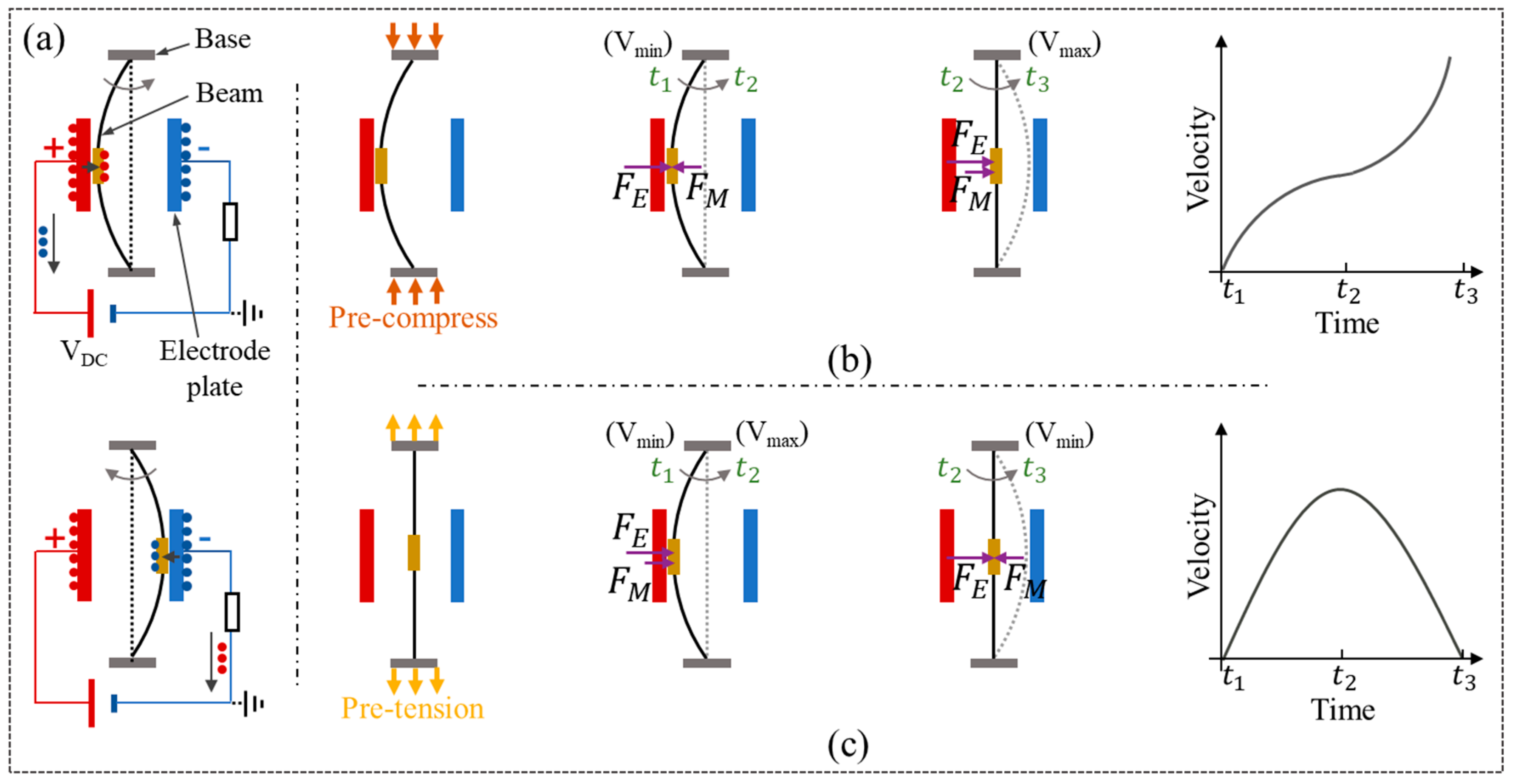
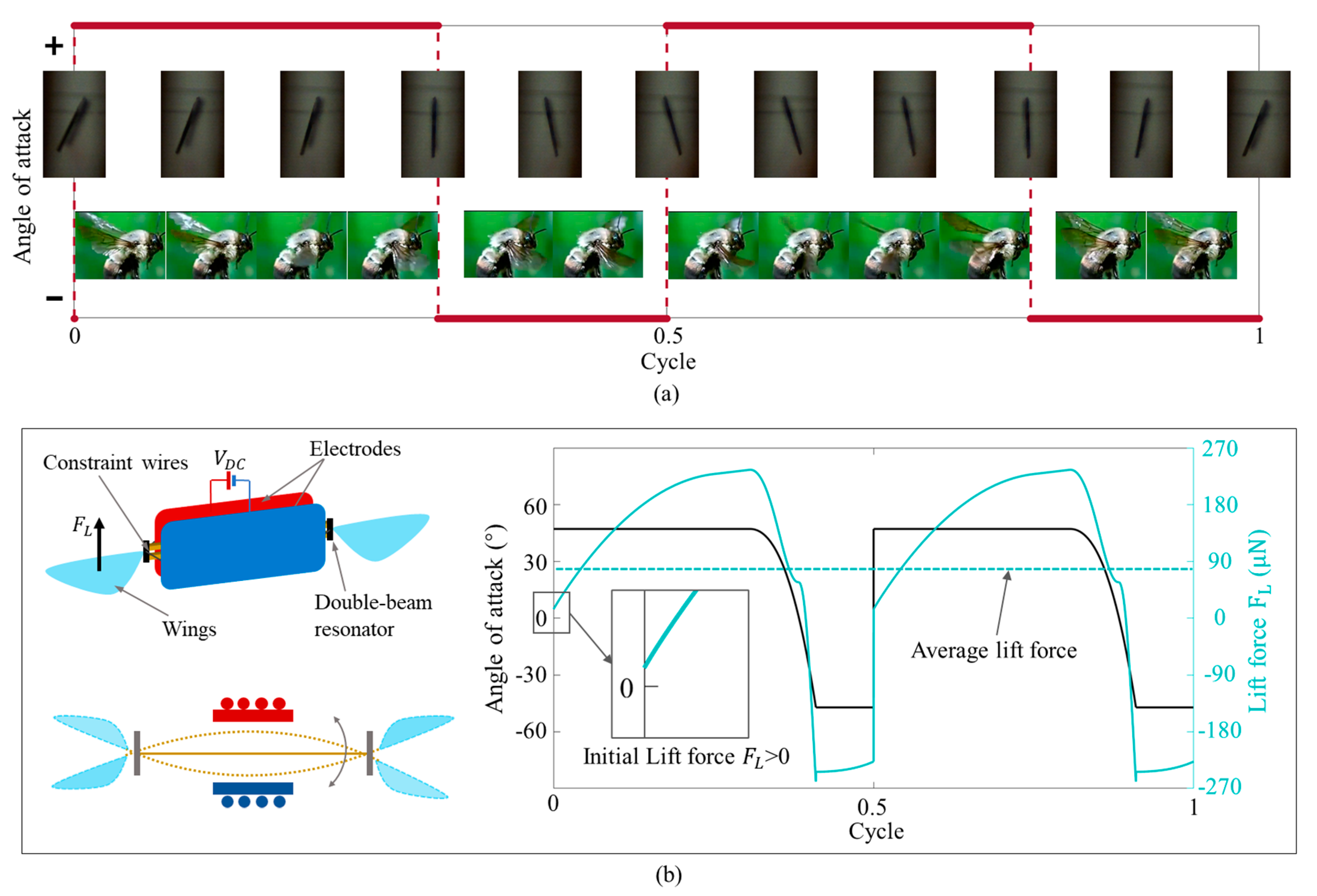
2.1. Structure and Principle
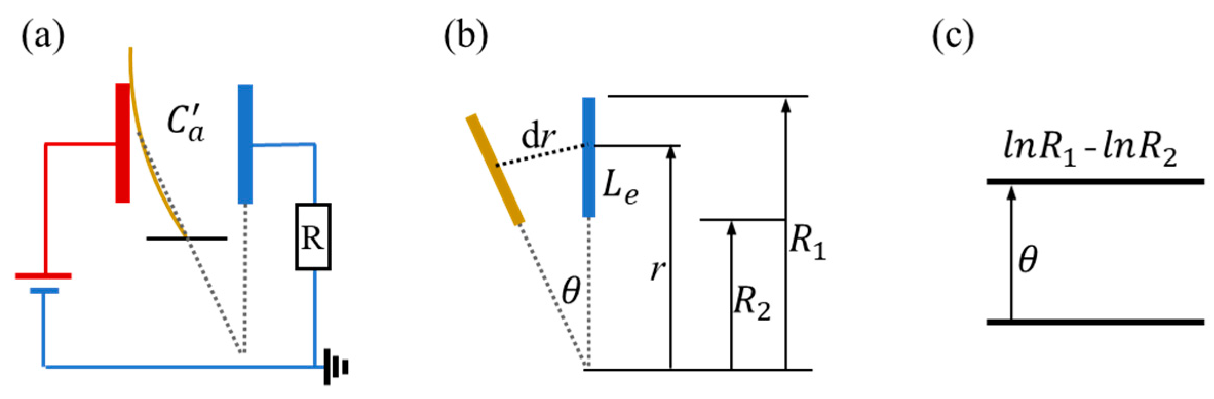
2.1.1. Electrostatic Force
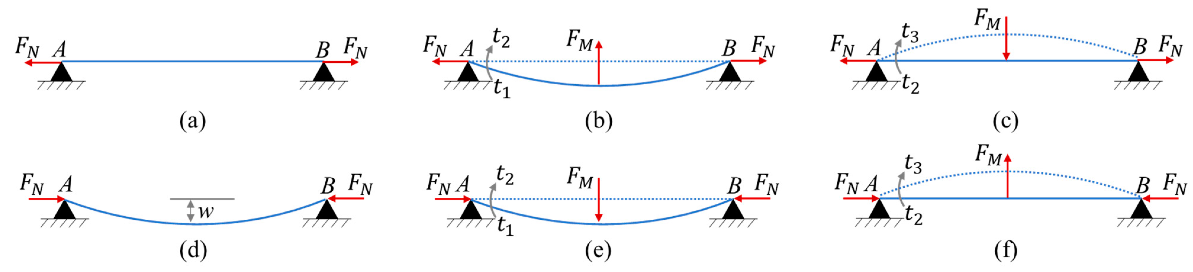
2.1.2. Quasi-Steady Analysis
2.1.3. Dynamic Model
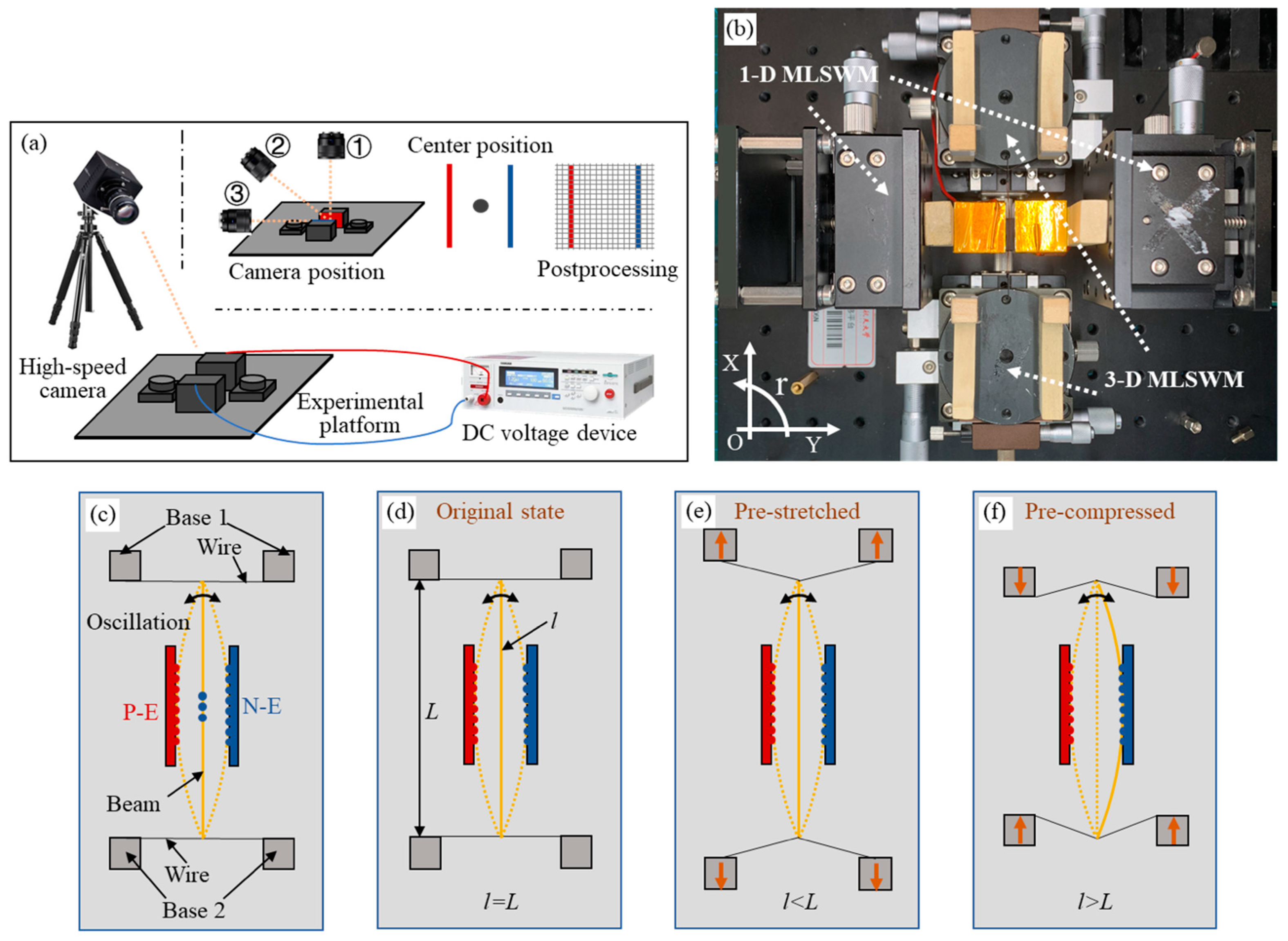
2.2. Experiment Setup
2.3. Measurement Setup for Oscillating Velocity of the Microbeam
3. Results
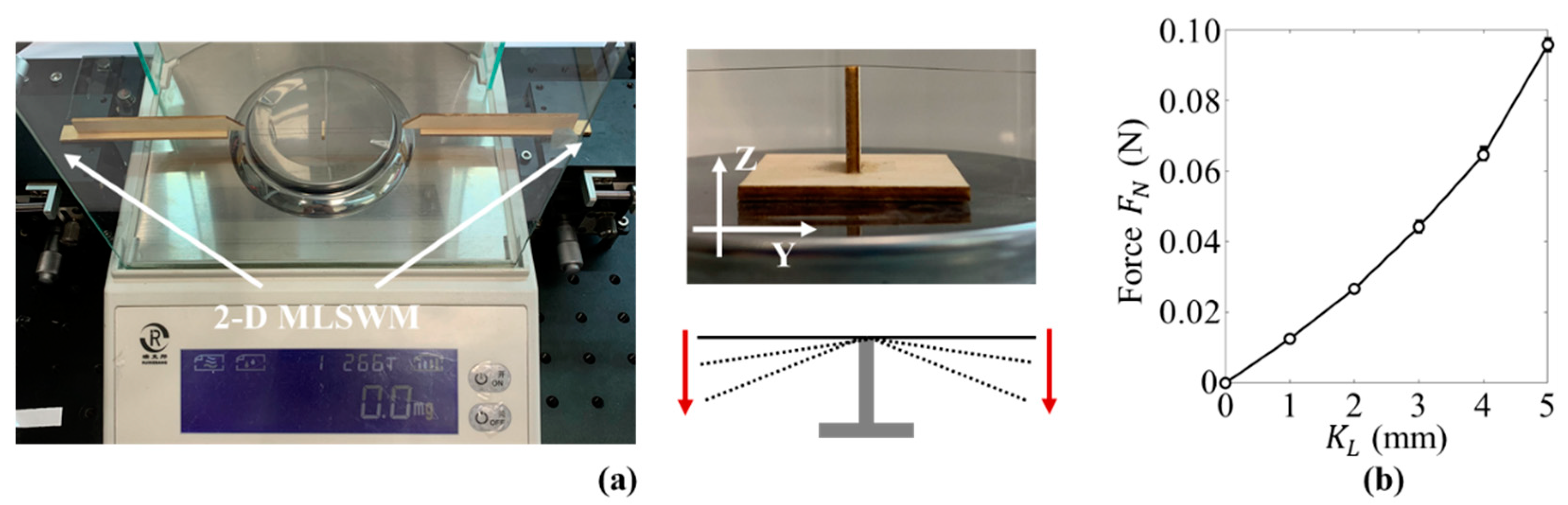
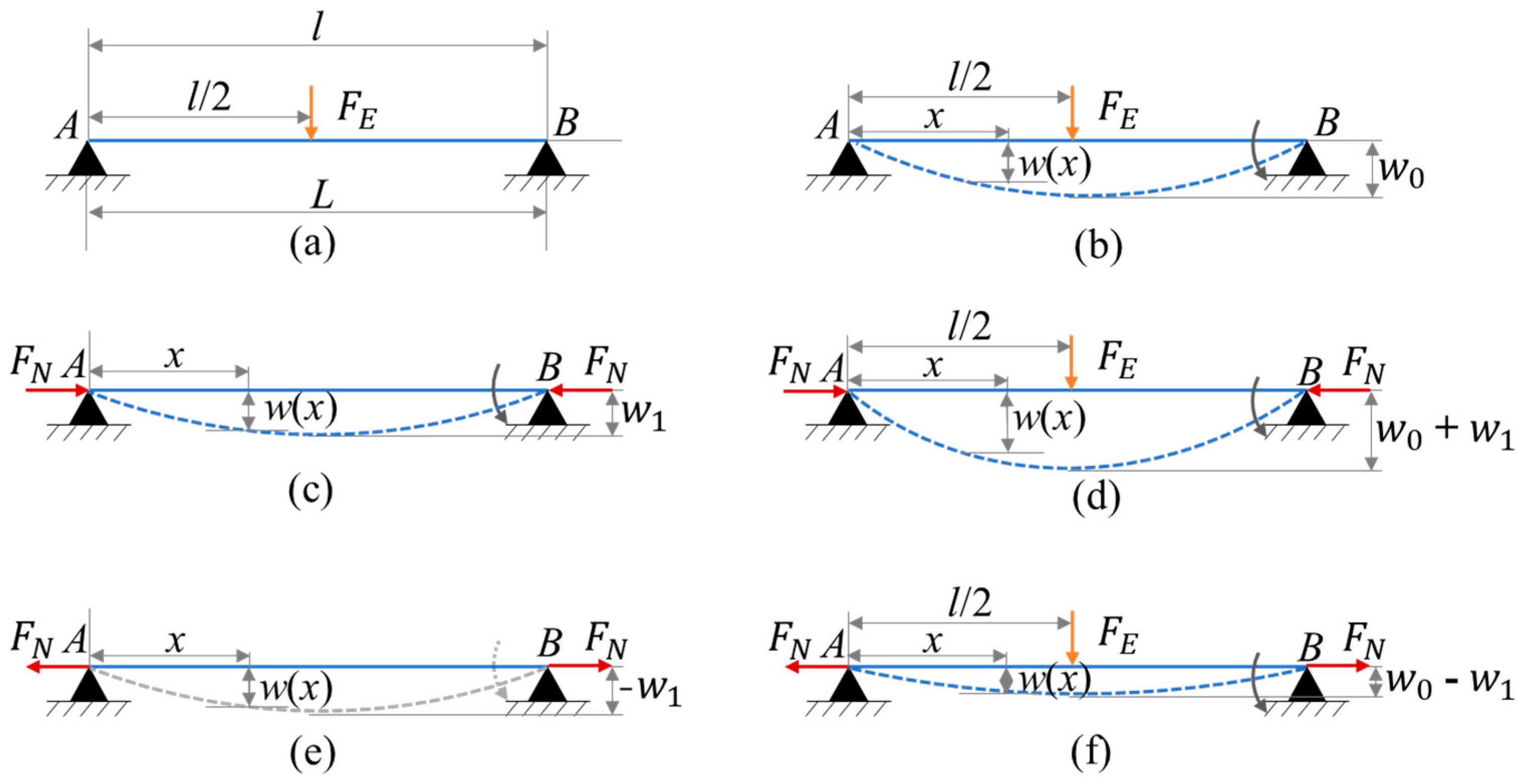
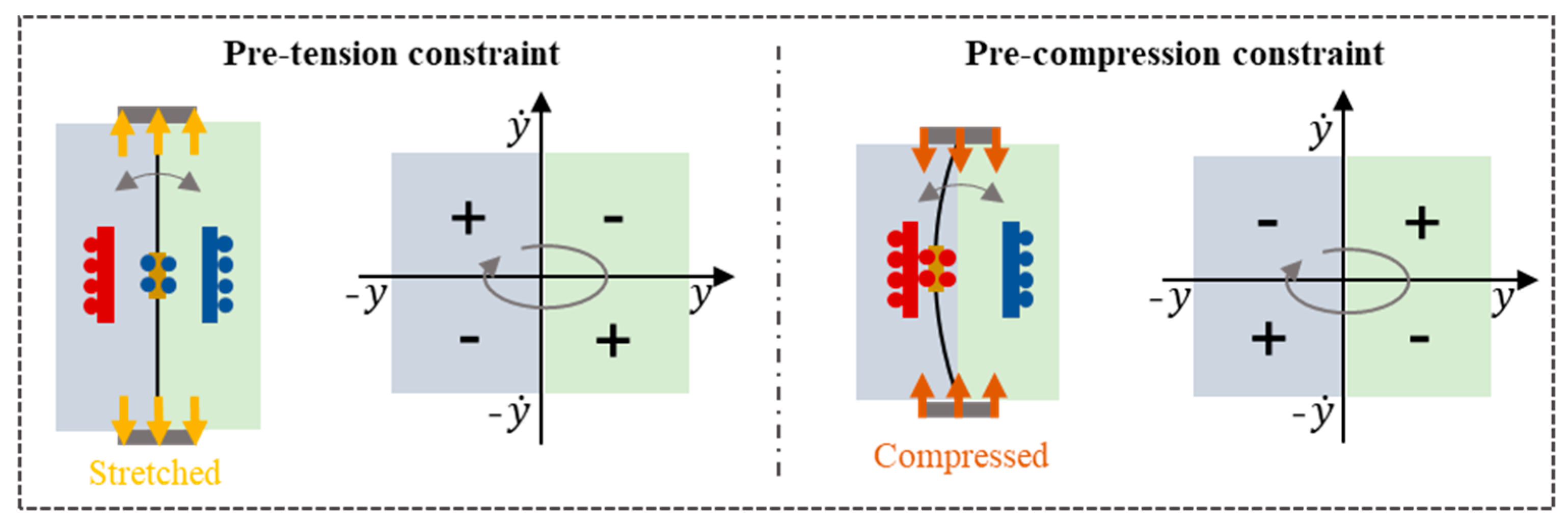
3.1. Variable Axial Restrain Force Caused by Different Pre-Constraints
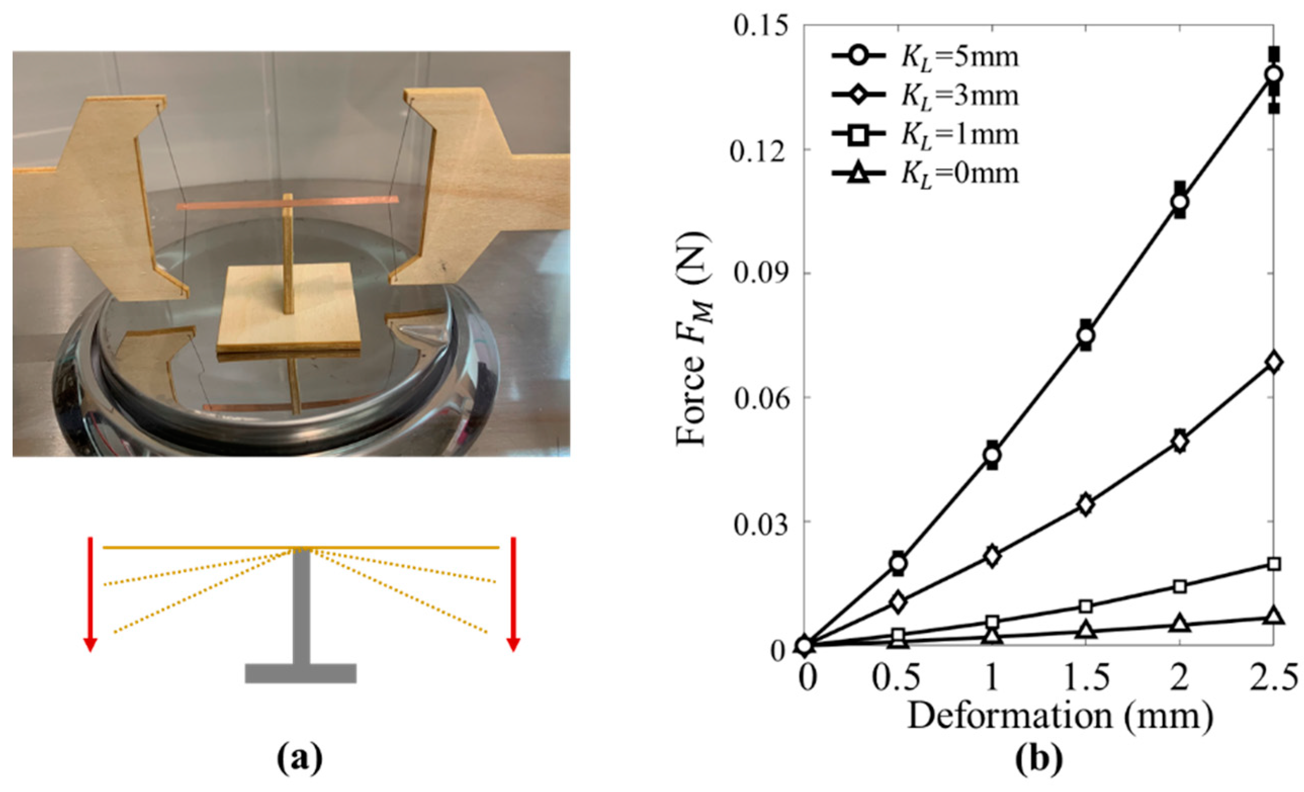
3.2. Variable Restoring Force Caused by Different Pre-Constraints
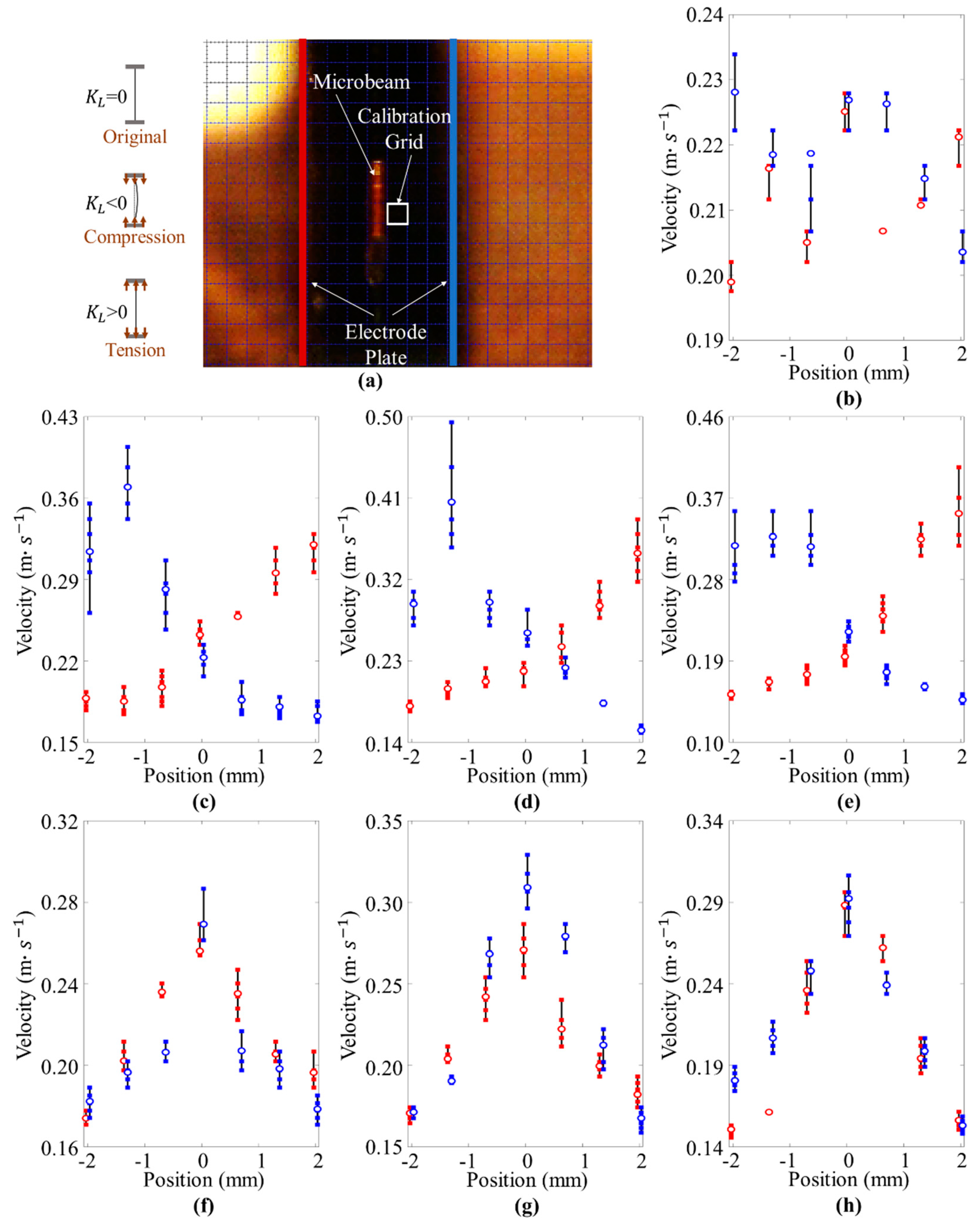
3.3. Variable Velocity-Position Characteristics Caused by Different Pre-Constraints
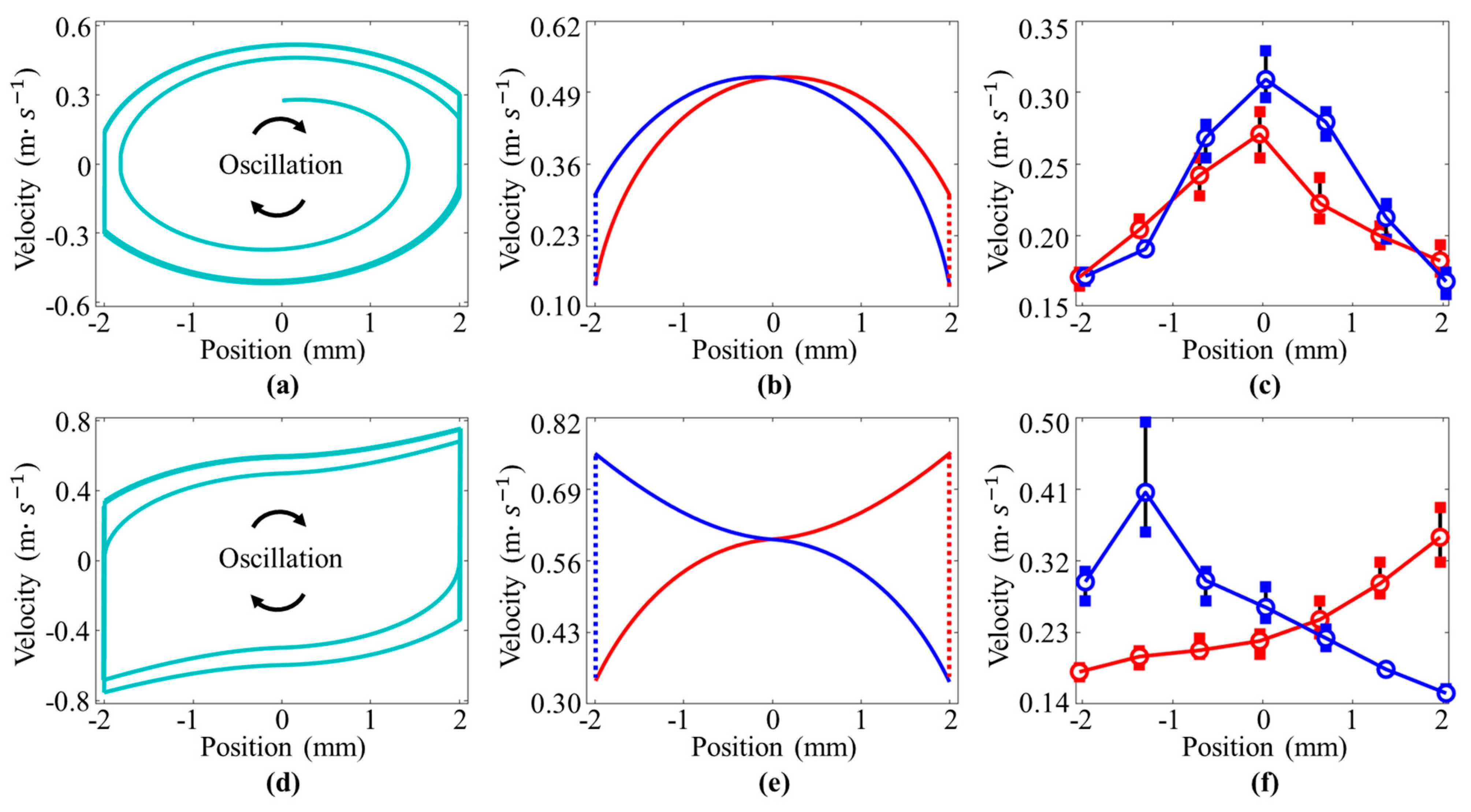
3.4. Oscillation Simulation
4. Discussion
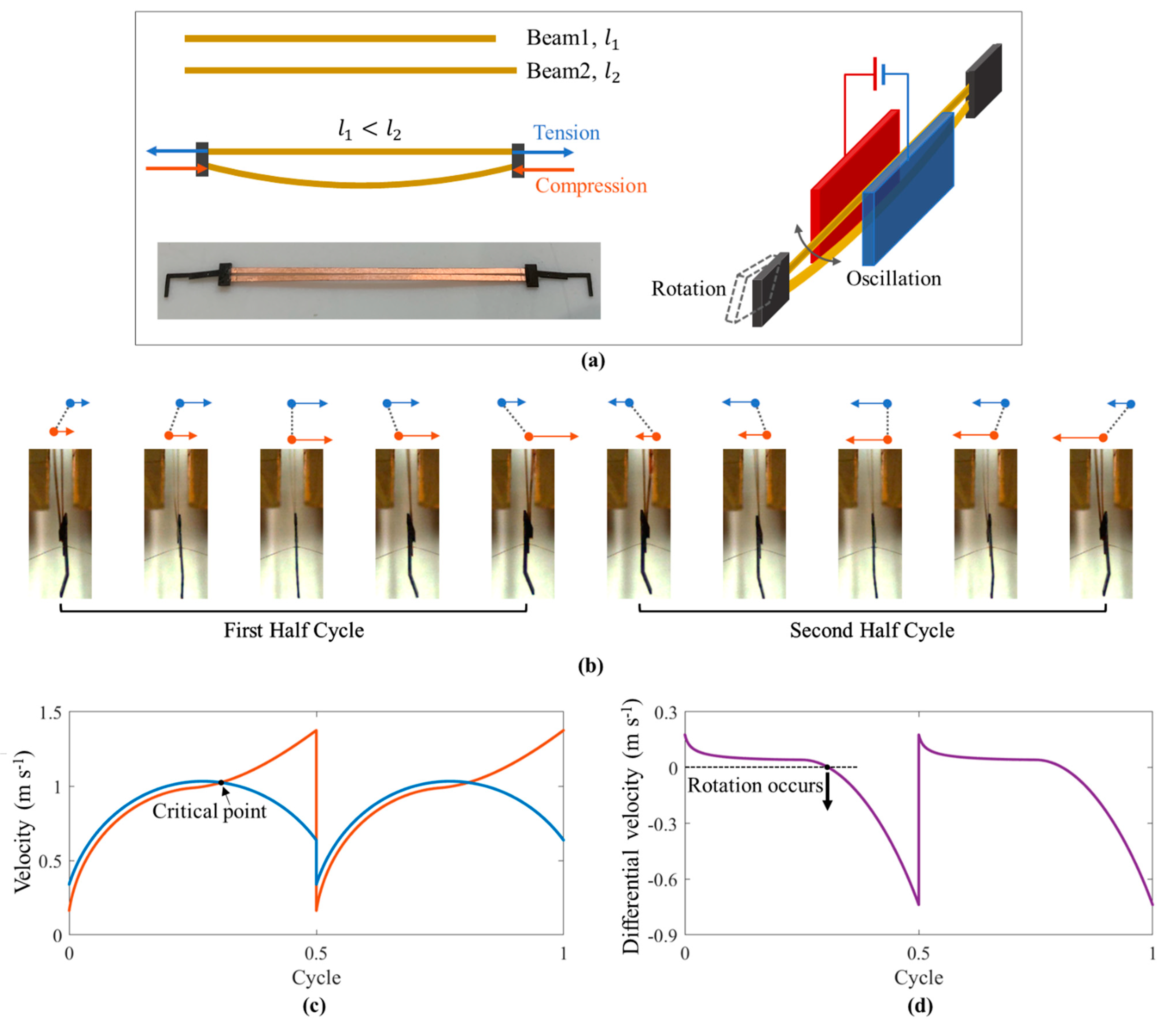
4.1. Differential Motion of the Double-Beam-Resonator
4.2. The Properties of the Double-Beam Resonator Compared to Others
4.3. Advanced Rotation Control of Flapping Wings
5. Conclusions
Supplementary Materials
Author Contributions
Funding
Conflicts of Interest
Appendix A. Calculation of Electrostatic Force


| Value | |
|---|---|
| Capacitance dielectric constant | 8.86 × |
| Microbeam width . | 3 × m |
| Electrode width | 20 × m |
| Half distance between the electrodes | 2 × m |
| Distance between the electrodes d | 4 × m |
| Electrode length | 20.4 × m |
| Beam length between electrodes | 20 × m |
| The angle between electrode and beam | 0.1 |
| The top radius of the beam | 40.0667 × m |
| The bottom radius of the beam | 20.0667 × m |
Appendix B. Different Stiffness Caused by the Pre-Constraint

| Value | |
|---|---|
| Microbeam width . | 3 × m |
| Beam length | 40 × m |
| Beam thickness | 50 × m |
| Material modulus of elasticity E | 11.9 × Pa |
| Cross-sectional moment of inertia | 1.5625 × |
Appendix C. Parameters for the Dynamic Model

References
- Ma, K.Y.; Chirarattananon, P.; Fuller, S.B.; Wood, R.J. Controlled Flight of a Biologically Inspired, Insect-Scale Robot. Science 2013, 340, 603–607. [Google Scholar] [CrossRef] [PubMed] [Green Version]
- Dickinson, M.H.; Lehmann, F.-O.; Sane, S.P. Wing Rotation and the Aerodynamic Basis of Insect Flight. Science 1999, 284, 1954–1960. [Google Scholar] [CrossRef] [PubMed]
- Sane, S.P.; Dickinson, M.H. The control of flight force by a flapping wing: Lift and drag production. J. Exp. Biol. 2001, 204, 2607–2626. [Google Scholar] [CrossRef] [PubMed]
- Chin, D.D.; Lentink, D. Flapping wing aerodynamics: From insects to vertebrates. J. Exp. Biol. 2016, 219, 920–932. [Google Scholar] [CrossRef] [PubMed] [Green Version]
- Lehmann, F.-O. The mechanisms of lift enhancement in insect flight. Naturwissenschaften 2004, 91, 101–122. [Google Scholar] [CrossRef] [PubMed]
- Khan, Z.A.; Agrawal, S.K. Design and Optimization of a Biologically Inspired Flapping Mechanism for Flapping Wing Micro Air Vehicles; IEEE: Piscataway, NJ, USA, 2007; pp. 373–378. [Google Scholar]
- Khan, Z.A.; Agrawal, S.K. Study of Biologically Inspired Flapping Mechanism for Micro Air Vehicles. AIAA J. 2011, 49, 1354–1365. [Google Scholar] [CrossRef]
- Azhar, M.; Campolo, D.; Lau, G.-K.; Hines, L.; Sitti, M. Flapping wings via direct-driving by DC motors. In 2013 IEEE International Conference on Robotics and Automation; IEEE: Piscataway, NJ, USA, 2013; pp. 1397–1402. [Google Scholar]
- Jafferis, N.T.; Helbling, E.F.; Karpelson, M.; Wood, R.J. Untethered flight of an insect-sized flapping-wing microscale aerial vehicle. Nat. Cell Biol. 2019, 570, 491–495. [Google Scholar] [CrossRef] [PubMed]
- Yan, X.; Qi, M.; Lin, L. An autonomous impact resonator with metal beam between a pair of parallel-plate electrodes. Sens. Actuators A Phys. 2013, 199, 366–371. [Google Scholar] [CrossRef]
- Liu, Z.; Yan, X.; Qi, M.; Lin, L. Electrostatic Flapping Wings with Pivot-Spar Brackets for High Lift Force; IEEE: Piscataway, NJ, USA, 2016; pp. 1133–1136. [Google Scholar]
- Qi, M.; Yang, Y.; Yan, X.; Liu, Z.; Zhu, Y.; Zhang, X.; Lin, L. Untethered flight of a tiny balloon via self-sustained electrostatic actuators. In Proceedings of the 2017 19th International Conference on Solid-State Sensors, Actuators and Microsystems (TRANSDUCERS), Kaohsiung, Taiwan, 18–22 June 2017; IEEE: Piscataway, NJ, USA, 2017; pp. 2075–2078. [Google Scholar]
- Dickinson, M.H.; Lighton, J. Muscle efficiency and elastic storage in the flight motor of Drosophila. Science 1995, 268, 87–90. [Google Scholar] [CrossRef] [PubMed] [Green Version]
- Madangopal, R.; Khan, Z.A.; Agrawal, S. Energetics-based design of small flapping-wing micro air vehicles. IEEE/ASME Trans. Mechatron. 2006, 11, 433–438. [Google Scholar] [CrossRef]
- Madangopal, R.; Khan, Z.A.; Agrawal, S.K. Biologically Inspired Design Of Small Flapping Wing Air Vehicles Using Four-Bar Mechanisms And Quasi-steady Aerodynamics. J. Mech. Des. 2004, 127, 809–816. [Google Scholar] [CrossRef] [Green Version]
- Zhang, C.; Rossi, C. A review of compliant transmission mechanisms for bio-inspired flapping-wing micro air vehicles. Bioinspiration Biomim. 2017, 12, 025005. [Google Scholar] [CrossRef] [PubMed]
- Wood, R.J. The First Takeoff of a Biologically Inspired At-Scale Robotic Insect. IEEE Trans. Robot. 2008, 24, 341–347. [Google Scholar] [CrossRef]
- Mateti, K.; Byrne-Dugan, R.A.; Rahn, C.D.; Tadigadapa, S.A. Monolithic SUEX Flapping Wing Mechanisms for Pico Air Vehicle Applications. J. Microelectromechanical Syst. 2012, 22, 527–535. [Google Scholar] [CrossRef]
- Deng, X.; Schenato, L.; Wu, W.C.; Sastry, S.S. Flapping flight for biomimetic robotic insects: Part I-system modeling. IEEE Trans. Robot. 2006, 22, 776–788. [Google Scholar] [CrossRef]
- Fenelon, M.A.; Furukawa, T. Design of an active flapping wing mechanism and a micro aerial vehicle using a rotary actuator. Mech. Mach. Theory 2010, 45, 137–146. [Google Scholar] [CrossRef]
- Ellington, C.P. The aerodynamics of hovering insect flight. I. The quasi-steady analysis. Philos. Trans. R. Soc. B Biol. Sci. 1984, 305, 1–15. [Google Scholar] [CrossRef]
- Palmer, H.B. The Capacitance of a Parallel-Plate Capacitor by the Schwartz-Christoffel Transformation. Trans. Am. Inst. Electr. Eng. 1937, 56, 363–366. [Google Scholar] [CrossRef]
- Hosseini, M.; Zhu, G.; Peter, Y.-A. A new formulation of fringing capacitance and its application to the control of parallel-plate electrostatic micro actuators. Analog. Integr. Circuits Signal Process. 2007, 53, 119–128. [Google Scholar] [CrossRef]


| Cycle | First Half Cycle | Second Half Cycle | ||||
|---|---|---|---|---|---|---|
| Position/mm | −2 | 0 | 2 | 2 | 0 | −2 |
| mm | 44.06 | 56.02 | 100 | 42.31 | 63.84 | 90.14 |
| mm | 45.34 | 55.04 | 87.16 | 38.62 | 65.31 | 73.44 |
| mm | 50.95 | 65.94 | 86.74 | 46.90 | 60.50 | 84.32 |
| mm | 87.25 | 98.73 | 97.01 | 89.24 | 99.49 | 100 |
| mm | 64.78 | 95.11 | 73.07 | 66.33 | 100 | 67.83 |
| mm | 55.47 | 87.84 | 59.10 | 54.42 | 100 | 55.68 |
| mm | 51.86 | 99.03 | 53.78 | 52.67 | 100 | 62.07 |
| Resonator Prototype | Simply Supported | Pre-Tension | Pre-Compression | Double-Beam |
|---|---|---|---|---|
| Velocity-Position Curve |  |  |  |  |
| Frequency | Low | High | High | High |
| Active Rotation | No | No | No | Yes |
Publisher’s Note: MDPI stays neutral with regard to jurisdictional claims in published maps and institutional affiliations. |
© 2021 by the authors. Licensee MDPI, Basel, Switzerland. This article is an open access article distributed under the terms and conditions of the Creative Commons Attribution (CC BY) license (https://creativecommons.org/licenses/by/4.0/).
Share and Cite
Yun, R.; Zhu, Y.; Liu, Z.; Huang, J.; Yan, X.; Qi, M. An Electrostatic Self-Excited Resonator with Pre-Tension/Pre-Compression Constraint for Active Rotation Control. Micromachines 2021, 12, 650. https://0-doi-org.brum.beds.ac.uk/10.3390/mi12060650
Yun R, Zhu Y, Liu Z, Huang J, Yan X, Qi M. An Electrostatic Self-Excited Resonator with Pre-Tension/Pre-Compression Constraint for Active Rotation Control. Micromachines. 2021; 12(6):650. https://0-doi-org.brum.beds.ac.uk/10.3390/mi12060650
Chicago/Turabian StyleYun, Ruide, Yangsheng Zhu, Zhiwei Liu, Jianmei Huang, Xiaojun Yan, and Mingjing Qi. 2021. "An Electrostatic Self-Excited Resonator with Pre-Tension/Pre-Compression Constraint for Active Rotation Control" Micromachines 12, no. 6: 650. https://0-doi-org.brum.beds.ac.uk/10.3390/mi12060650