Article

Ex Vivo High-Resolution Magic Angle Spinning (HRMAS) 1H NMR Spectroscopy for Early Prostate Cancer Detection

1
Department of Pathology, Harvard Medical School/Massachusetts General Hospital, Boston, MA 02114, USA
2
Department of Diagnostic and Interventional Radiology, University Hospital Ulm, 89081 Ulm, Germany
3
Radiology Gotha, SRH Poliklinik Gera, 99867 Gotha, Germany
4
SRH University of Applied Health Sciences, 07548 Gotha, Germany
5
Department of Urology, Harvard Medical School/Massachusetts General Hospital, Boston, MA 02114, USA
6
i2SouI—Innovative Imaging in Surgical Oncology Ulm, University Hospital Ulm, 89081 Ulm, Germany
7
Center for Translational Imaging “From Molecule to Man” (MoMan), University Hospital Ulm, 89081 Ulm, Germany
8
Comprehensive Cancer Center Ulm (CCCU), University Hospital Ulm, 89081 Ulm, Germany
9
Departments of Pathology and Radiology, Harvard Medical School/Massachusetts General Hospital, Boston, MA 02114, USA
*
Author to whom correspondence should be addressed.
Submission received: 25 March 2022 / Revised: 17 April 2022 / Accepted: 22 April 2022 / Published: 26 April 2022
(This article belongs to the Special Issue Cancer Metabolomic Analysis)

Abstract

:

Simple Summary

Prostate cancer is the second leading cancer diagnosed in men worldwide. Current diagnostic standards lack sufficient reliability in detecting and characterizing prostate cancer. Due to the cancer’s multifocality, prostate biopsies are associated with high numbers of false negatives. Whereas several studies have already shown the potential of metabolomic information for PCa detection and characterization, in this study, we focused on evaluating its predictive power for future PCa diagnosis. In our study, metabolomic information differed substantially between histobenign patients based on their risk for receiving a future PCa diagnosis, making metabolomic information highly valuable for the individualization of active surveillance strategies.

Abstract

The aim of our study was to assess ex vivo HRMAS (high-resolution magic angle spinning) 1H NMR spectroscopy as a diagnostic tool for early PCa detection by testing whether metabolomic alterations in prostate biopsy samples can predict future PCa diagnosis. In a primary prospective study (04/2006–10/2018), fresh biopsy samples of 351 prostate biopsy patients were NMR spectroscopically analyzed (Bruker 14.1 Tesla, Billerica, MA, USA) and histopathologically evaluated. Three groups of 16 patients were compared: group 1 and 2 represented patients whose NMR scanned biopsy was histobenign, but patients in group 1 were diagnosed with cancer before the end of the study period, whereas patients in group 2 remained histobenign. Group 3 included cancer patients. Single-metabolite concentrations and metabolomic profiles were not only able to separate histobenign and malignant prostate tissue but also to differentiate between samples of histobenign patients who received a PCa diagnosis in the following years and those who remained histobenign. Our results support the hypothesis that metabolomic alterations significantly precede histologically visible changes, making metabolomic information highly beneficial for early PCa detection. Thanks to its predictive power, metabolomic information can be very valuable for the individualization of PCa active surveillance strategies.

1. Introduction

Prostate cancer (PCa) is the second most frequently diagnosed cancer and the fifth most frequent cause of cancer-related deaths in men worldwide [1], thus representing a tremendous burden for public health systems. So far, the detailed etiology of PCa remains largely unexplained, with only a few established risk factors, including age, positive family history and ethnic origin [2].
At present, one of the most urging challenges in PCa diagnostics and therapy is the precise differentiation between patients with highly aggressive tumors and those with indolent tumors [3,4]. This distinction is essential for deciding on adequate, stage-adapted therapy strategies. Whereas patients with malignant tumors should immediately receive a curative therapy, those with indolent forms need protection from overtreatment with invasive therapies [3,4,5]. A transrectal ultrasound (TRUS)-guided systematic needle biopsy followed by histopathological evaluation is the current gold standard in PCa diagnostics [6]. Histopathological grading of prostate tumors, an important prognostic indicator, regularly follows the Gleason system [7,8].
The introduction of prostate-specific antigen (PSA) screening and an increase in prostate biopsy samples from 6 to 12 both resulted in a substantial rise in early-stage PCa diagnoses [9,10], indicating an essential need for higher diagnostic accuracy and more precise malignancy differentiation in early cancer detection [11]. Although PSA is used as a tumor marker and screening parameter, it is not tumor- but only prostate-specific [12] and, apart from intraindividual variations, can rise in the context of several circumstances other than PCa, such as benign prostatic hyperplasia, prostatitis or other manipulations of the prostate [12,13].
Additionally, with prostate tumors usually showing multifocal growth behavior [14], a significant number of cancer foci remains undetected during prostate biopsies, and tumor aggressiveness is often underestimated [14,15].
To summarize, current PCa diagnostic standards lack sufficient accuracy, as well as reliability, in distinguishing indolent from aggressive tumors. Therefore, in order to satisfy the requirement for personalized tumor- and stage-adapted therapy, more reliable screening strategies, diagnostic methods and biomarkers are needed [11].
HRMAS 1H NMR spectroscopy is among the diagnostic methods that have been investigated for this cause. It enables the ex vivo analysis of tissue samples with sufficient spectral resolution by spinning them at an angle of 54.7° away from the direction of the spectrometer’s static magnetic field [11,16]. Moreover, tissue structure preservation during NMR experiments allows for subsequent histopathological and genetic evaluation of samples [17,18] and, thus, the analysis of correlations between tissue metabolites and pathologies [18].
Therefore, metabolite quantification with ex vivo HRMAS 1H NMR spectroscopy represents a promising tool for investigating biochemical processes underlying PCa development and progression. The metabolome composition, meaning the entirety of all measurable metabolites [19,20], changes dynamically as the biological system reacts to genetic and environmental stimuli, such as diseases like cancer [19,20]. Specific metabolomic alterations are characteristic of malignant tumor cells [21], making the evaluation of cancer-specific metabolomic profiles diagnostically extremely valuable [11,22]. In several studies, metabolomic information acquired with ex vivo NMR spectroscopy has shown its potential for PCa detection, characterization and prognostic evaluation [22,23,24]. In this context, it was shown that the analysis of metabolomic profiles has superior accuracy compared to that of single metabolites [11,24].
Several authors suggested that metabolomic alterations significantly precede histologically visible changes [11,25]. Consequently, metabolomic information might be highly beneficial for the analysis of early prostate cancer development and behavior [11]. However, to our knowledge, no work exists that has examined individual metabolite concentrations and metabolomic profiles in histobenign samples and correlated them with later evolution (development of carcinoma vs. persistently benign).
Based on this assumption, the purpose of our study was to evaluate the diagnostic value of ex vivo NMR spectroscopy for early PCa detection by correlating metabolomic information with histopathology. In particular, we focused on assessing the predictive potential of metabolomic alterations in prostate biopsy samples of histobenign patients for a prostate cancer diagnosis in the following years. The aim was to answer the question of whether metabolomic data can separate a group of histobenign patients into two subgroups according to their risk for a future malignant transformation. A further object of this study was the differentiation of Gleason score (GS) categories 3 + 3 = 6 and 3 + 4 = 7 based on metabolite concentrations. Moreover, we wanted to evaluate whether there are linear correlations between metabolite intensities/metabolomic profiles and the PSA density (PSAd) as well as the volume percentage of benign epithelium in the tissue sample (Vol.%Epi).

2. Materials and Methods
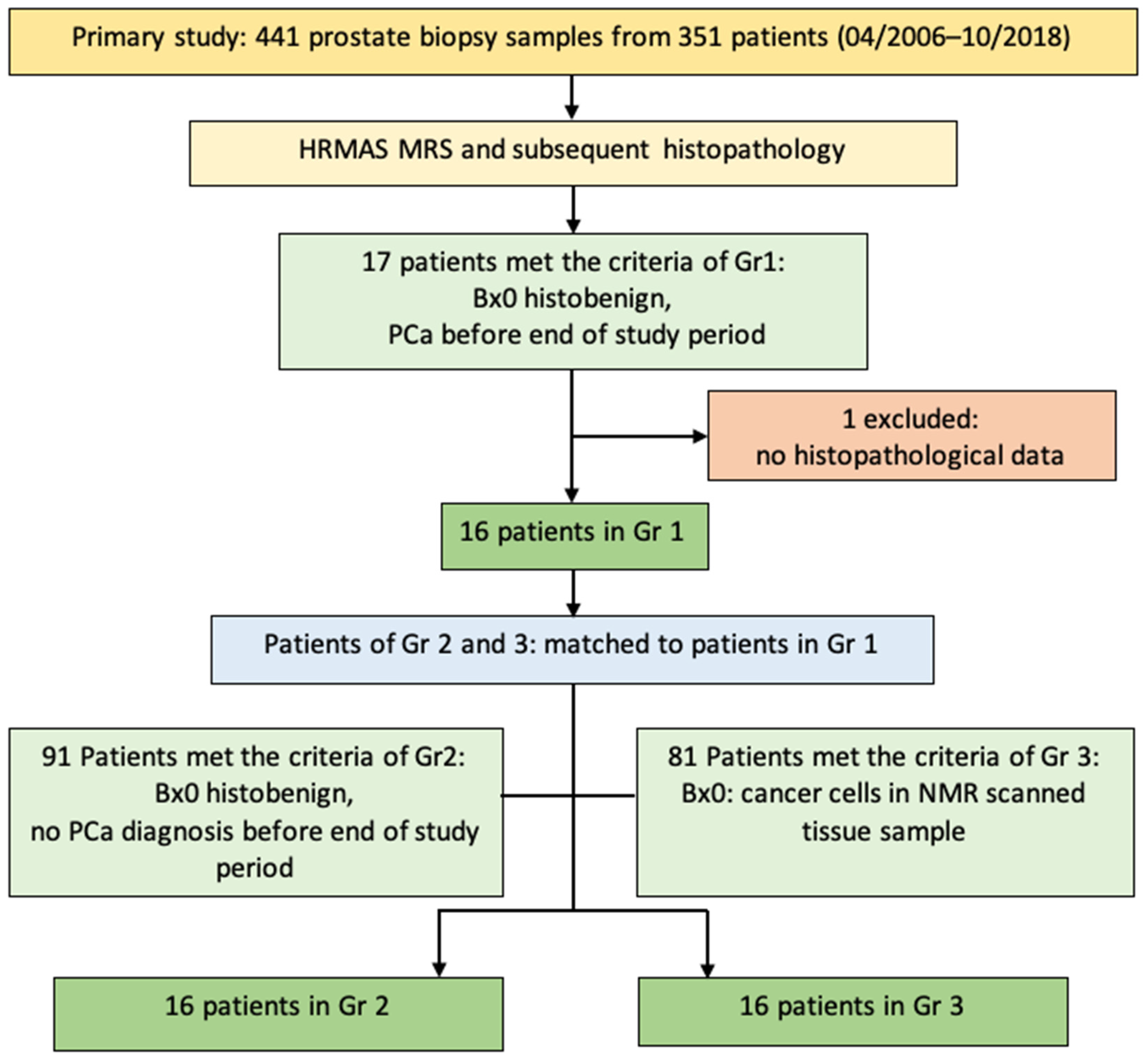
2.1. Patients

This study is part of a primary prospective study. Before its start in 2006, an independent ethics committee, the Partners Human Research Committee Institutional Review Board, reviewed and approved the study (Protocol #: 2005P000892), and it was conducted according to specified rules and guidelines. Patients who underwent a prostate biopsy at the MGH Urology Department were considered for the study and only included after having given their written informed consent. From April 2006 until October 2018, 441 prostate tissue samples from 351 patients were progressively included in the study (90 patients participated with two prostate tissue samples each).
Clinical and pathological patient data were obtained from the Epic Partners patient database (Partners HealthCare International, Boston, MA, USA), including the following parameters: age at biopsy Bx0 (biopsy during which the NMR scanned sample(s) was/were taken), pre-Bx0 PSA, pre-Bx0 PSA density, prostate volume, American Joint Committee on Cancer Pathological Tumor Stage pTNM (in case of post-prostatectomy patients), GS of Bx0 (overall GS and GS of the NMR-analyzed sample(s)) and highest GS of all biopsies until the end of the study period.
With regard to our research question, we performed a subgroup analysis of all 351 patients and built three homogenous groups of 16 patients (Gr): Gr1 and 2 included patients whose NMR scanned biopsy (Bx0) was histobenign, but Gr1 patients received a PCa diagnosis before the end of the study period, whereas Gr2 patients remained histobenign. NMR scanned biopsy samples of Gr3 already included cancer cells. The subgroup analysis included matching patients 1–16 of Gr2 and 3 to patients 1–16 of Gr1, following predefined clinical and histopathological matching criteria (pTNM for patients who underwent a prostatectomy, GS, PSAd, age at Bx0) (Figure 1).

2.2. Intact Tissue Magnetic Resonance Spectroscopy (MRS)

During a patient’s biopsy, 1–2 additional tissue samples were taken for the study and analyzed with HRMAS 1H NMR spectroscopy on a Bruker Avance 600 MHz (14.1 Tesla) spectrometer (Bruker BioSpin Corp., Billerica, MA, USA) on the same day. Tissue cores were analyzed in a fresh, unfrozen state. Therefore, in order to prevent them from drying out and to minimize potential degradation of tissue metabolites, samples were placed in a construction of tubes functioning as a humidity chamber and stored on ice until the NMR experiment, as recommended by Tilgner et al. [26].
All spectrometer analyses were conducted according to the same protocol and without any knowledge of the clinical patient conditions. Tissue samples were placed into a 4 mm long rotor; then, 10 µL D2O (Sigma Aldrich, St. Louis, MO, USA) was added for field-locking. The spectra recording conditions were set as follows: temperature = 4 °C, repetition time = 5 s and the spectrometer resonance centered on the water resonance. A rotor-synchronized DANTE protocol with spinning rates of both 600 and 700 Hz for each sample was applied.
HRMAS NMR data were first processed and analyzed with a lab-intern MatLab program (MathWorks, Natrick, MA, USA, Version 2009b). Integrals of spectral peaks in the range from 0.5 to 4.5 ppm (parts per million of magnetic field strength) were calculated using spectral curve fittings with Lorentzian–Gaussian line shapes and represented spectral peak intensities. Regions containing alcohol peaks and therefore indicating a potential contamination with biopsy gel were excluded from further analysis. The spectral range from 0.5 to 4.5 ppm was divided into 58 regions (Reg.), and spectral peak intensities were summed up to regional peak intensities (see Table A1 in Appendix A, which shows the spectral regions and their assigned ppm values). Regions were defined according to the spectral shape and a specific mathematical procedure with the aim of assigning whole peaks to one region and preventing peaks from being split up in between different regions. Spectral processing was verified in Acorn-NMR-Nuts (Livermore, CA, USA, 2D Professional version) in order to ensure the MATLab algorithm detected and integrated all peaks. Normalized spectral peak intensities were calculated for each region for better comparability of tissue samples within the study population. An outlier analysis of the spectral peak intensities was performed by calculating the Mahalanobis distance for each regional spectral peak intensity in SAS-JMP, with an upper control limit of 1.94. Metabolites and ppm values were assigned according to the literature (see Table A2 in Appendix B, which displays the assignment of metabolites to spectral regions), with peaks representing the signal of metabolites and peak intensities their concentrations. As regional peak intensities were compared instead of specific metabolites, it is possible that more than one metabolite contributed to the signal in a given region. Only those metabolites that, according to the literature, have a large contribution to a certain region and are likely associated with prostate cancer are further discussed in this study.

2.3. Quantitative Histopathology

After the HRMAS MRS analysis, tissue samples were histopathologically evaluated. First, they were fixed in 10% formalin and then embedded in paraffin. Afterwards, 5 µm sections were cut off the biopsy sample at 100 µm intervals throughout the sample and then stained with hematoxylin-eosin. Two genitourinary pathologists with considerable experience in the evaluation of prostate cancer tissue (18 and 9 years, respectively) conducted all histopathological analyses. They microscopically estimated the percentage area representing stroma, benign epithelium (incl. lumens) and cancerous tissue (incl. lumens) (rounded off to the nearest 5%). The volume percentage of each tissue type was calculated by multiplying the area percentage by the area size of the tissue slice. Moreover, each tissue slice containing cancer cells was also evaluated using the Gleason system. In accordance with the definition of our study groups, biopsy samples of 32 patients (Gr1 and 2) were histobenign, and those of 16 patients contained cancer cells.

2.4. Statistical Analysis

Statistical tests were carried out in SAS JMP (Cary, NC, USA, Version JMP PRO 14) using the normalized spectral peak intensities calculated for 58 spectral regions and the first 12 principal components (PC). First, Shapiro–Wilks tests were performed to test for normal distribution. In order to analyze the data further, the following tests were performed: (1) analysis of variance (ANOVA) (normally distributed data) or Kruskal–Wallis–Wilcoxon test (non-normally distributed data) for the comparison of non-binary categorical variables (regional spectral peak intensities or PCs between all three groups); (2) student’s t-test (normally distributed data) or Mann–Whitney–Wilcoxon test (non-normally distributed data) for the comparison of binary categories (regional peak intensities and PCs between two groups, Gleason Score categories GS 3 + 3 = 6 and GS 3 + 4 = 7); (3) matched-pair analysis using a T test for paired data (normally distributed data) or the Wilcoxon signed-rank test (non-normally distributed data) for the comparison of regional spectral peak intensities between the matched pairs of two groups; (4) linear regressions of regional spectral peak intensities against the continuous variables Vol.%Epi and PSAd. Additionally, a multivariate analysis of covariance (MANCOVA) was performed in SPSS (IBM SPSS Statistics, Version 26, Armonk, NY, USA) in order to evaluate the effect of the variables age, PSAd and Vol.%Epi on the spectral peak intensities. The two-sided significance level for all statistical tests was set to α = 0.05.

3. Results

3.1. Clinical and (Histo)Pathological Patient Data

Overall, prostate biopsy samples of 48 patients (one sample each) were evaluated NMR spectroscopically and histopathologically in this study. Baseline characteristics are listed in Table 1, with further patient data in Table 2 and results from the histopathological evaluation in Table 3.

3.2. Differences between Histobenign and Malignant Prostate Tissue

The following paragraphs only address the most relevant results. All significant results and p-values can be found in Table A3, Table A4, Table A5, Table A6 and Table A7 in Appendix C.
Peak intensities of several spectral regions were able to significantly differentiate between Gr2 and 3 and therefore histobenign and malignant prostate tissue, such as Reg. 23 (3.05–3.08 ppm; p = 0.0052), the peak intensity of which typically contains the signal of polyamines. Moreover, a principal component named PC 6 was also able to separate Gr2 and 3 (p = 0.0332). Therefore, in addition to single metabolites, a metabolomic profile was able to distinguish between histobenign and malignant prostate tissue.

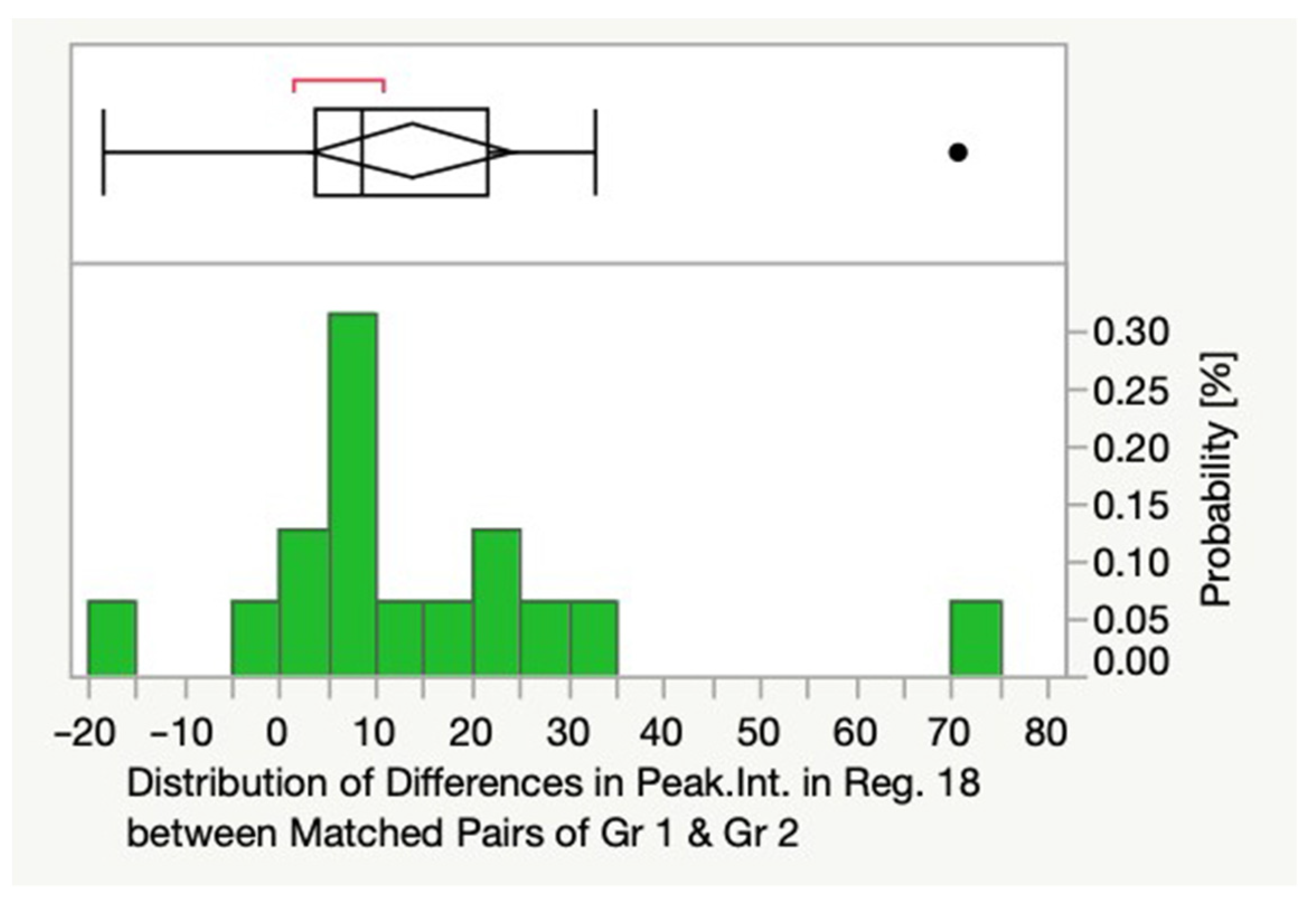
3.3. Differences between Histobenign and Premalignant Prostate Tissue

Peak intensities of several spectral regions and a principal component named PC 11 (p = 0.0365) were able to differentiate between Gr1 and 2 and therefore histobenign prostate tissue from patients who received a PCa diagnosis in the following years and those who remained histobenign. Reg. 18 (3.30–3.35 ppm; p = 0.0027) was one of these regions, with the signal of glycerophosphoethanolamine typically contributing to its peak intensity (Figure 2).

3.4. Differences between Premalignant and Malignant Prostate Tissue

Peak intensities of several spectral regions and a principal component called PC 1 (p = 0.0110) were able to distinguish between Gr1 and Gr3 and therefore premalignant and malignant prostate tissue. One example is Reg. 35 (2.30–2.38 ppm, p = 0.0092), which usually includes the signal of glutamate.

3.5. Differences between Gleason Score Categories GS 3 + 3 = 6 and 3 + 4 = 7

Peak intensities of several spectral regions were able to separate Gleason score categories GS 3 + 3 = 6 and 3 + 4 = 7, e.g., Reg. 27 (2.8–2.86 ppm; p = 0.0206), the peak intensity of which usually contains the signal of polyunsaturated fatty acid n-6 (PUFA n-6), and Reg. 23 (3.05–3.08 ppm; p = 0.0479), which usually represents the resonance of polyamines. This shows that metabolite intensities vary significantly according to Gleason score category.

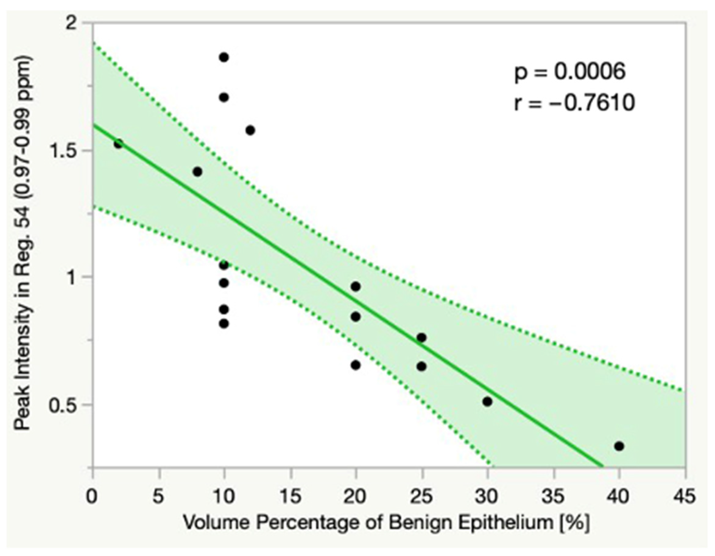
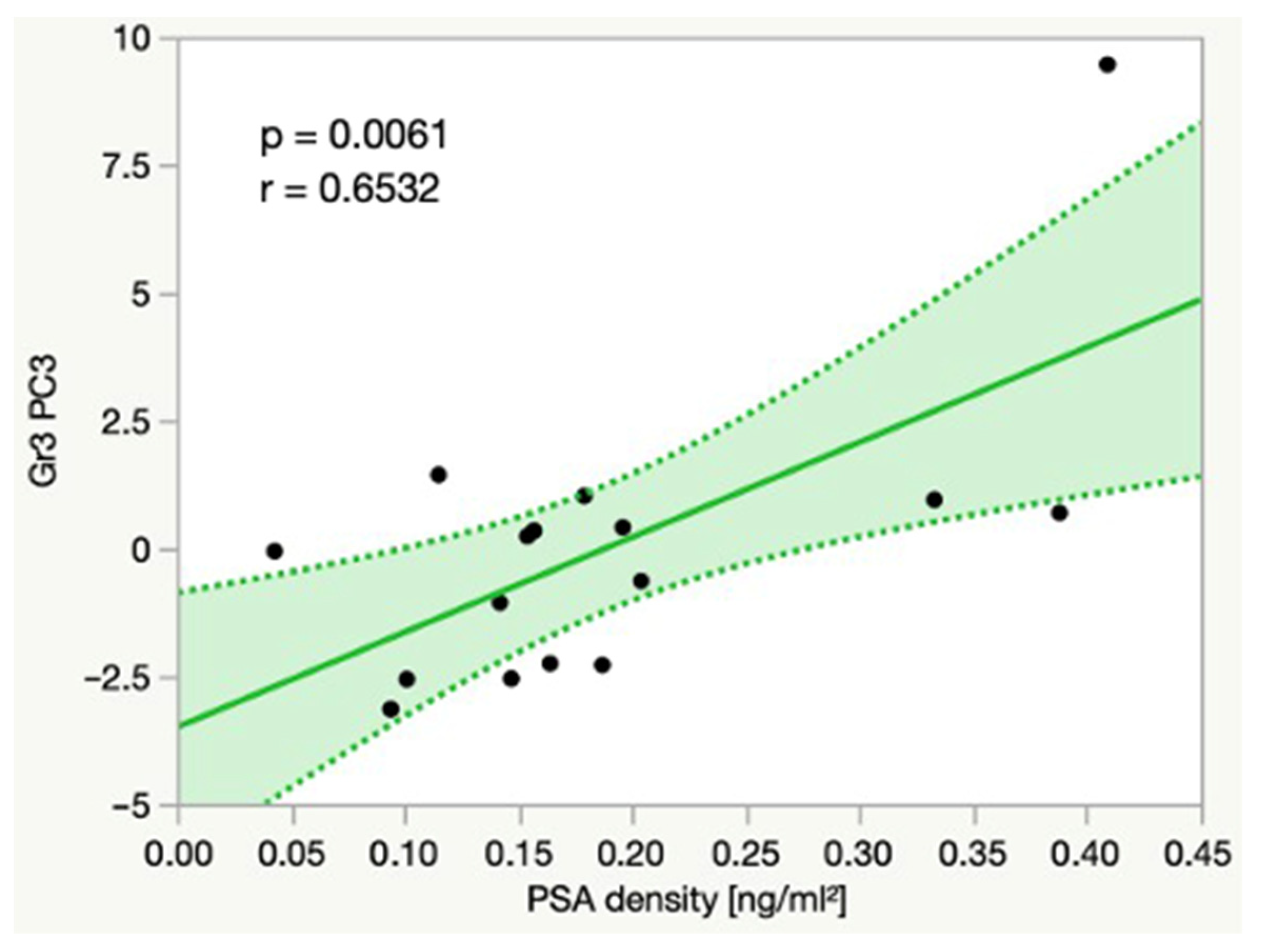
3.6. Linear Correlations

The volume percentage of benign epithelium correlated significantly with the spectral peak intensities in several regions. For example, we found a significant positive linear correlation between the Vol.%Epi and the spectral peak intensity in Reg. 30 (2.64–2.68 ppm; p = 0.0008, r = 0.4670) in all groups (Figure 3). Typically, the signal of citrate largely contributes to the peak intensity in this region. Moreover, there was a significant positive linear correlation between the Vol.%Epi and the spectral peak intensity in Reg. 23 (3.05–3.08 ppm; p = 0.0399, r = 0.2976), which usually represents the signal of polyamines.
In Gr1, there was a significant positive linear correlation between the Vol.% Epi and Reg. 16 (3.63–3.65 ppm; p = 0.0095, r = 0.6257), with the signal of myo-inositol (MI) as a typical contributor to its peak intensity. In Gr1, there was also a significant negative linear correlation between the Vol.%Epi and the principal components P10 (p = 0.0304, r = −0.5411) and P11 (p = 0.0414, r = −0.5146).
In Gr3, we found a significant negative linear correlation between the Vol.%Epi and the peak intensity in Reg. 54 (0.97–0.99 ppm; p = 0.0006, r = −0.7610), which usually contains the signals of isoleucine, leucine and valine (Figure 4).
Additionally, we were able to show significant linear correlations between the PSA density and multiple principal components, as well as the peak intensities of several spectral regions. For example, in Gr3, there was a significant positive linear correlation between the PSA density and Reg. 53 (1.00–1.06 ppm, p = 0.0047, r = 0.6682), which typically contains the signal of valine. In Gr3, the PSA density also significantly correlated with a principal component named PC3 (p = 0.0061, r = 0.6532) (Figure 5).

4. Discussion

The major aim of our study was to evaluate metabolomic information as a biomarker for early PCa detection. However, in addition to confirming differences in metabolite intensities and metabolomic profiles between histobenign and malignant prostate tissue, we wanted to assess whether metabolomic information significantly differs between histobenign patients who received a PCa diagnosis before the end of the study period and those who remained histobenign. This predictive power of metabolomic alterations in prostate biopsy samples of histobenign patients could be very useful for the identification of patients at high risk of a future PCa diagnosis, as well as the individualization of active surveillance strategies based on a patient’s metabolomic risk profile.

4.1. Differentiation between Histobenign, Premalignant and Malignant Prostate Tissue

In our study, the peak intensity in Reg. 23, which usually has contributions from the signal of polyamines, was significantly different between Gr2 and Gr3. Consequently, the concentration of polyamines seems to vary significantly between histobenign and cancerous prostate tissue. Healthy prostatic epithelial cells produce and secrete high amounts of spermine, a function that is progrediently lost with malignant transformation [27]. Our results are in accordance with those of Swanson [28,29] who detected significantly higher polyamine values in histobenign compared to malignant prostate tissue with HRMAS MRS.
Furthermore, the peak intensity in Reg. 18 significantly differentiated between histobenign prostate tissue of patients who remained histobenign and of those who received a PCa diagnosis in the following years (Gr2 and Gr1). The signals of gylcerophosphoethanolamine (GPhE) and scyllo-inositol (SI) usually fall in this region. GPhE is involved in cell membrane metabolism, which is accelerated during carcinogenesis, resulting in higher GPhE concentrations [30]. Changes in the metabolism of SI and MI have also been discussed in this context [25,30,31]. According to our results, we can assume that the GPhE metabolism and the SI metabolism already change in a premalignant, histologically not yet visible stage of early prostate carcinogenesis. SI and GPhE concentrations measured with HRMAS MRS could thus function as indicators of early PCa development in histobenign prostate tissue. Swanson et al. [32] also investigated phosphoethanolamine metabolism in PCa with HRMAS MRS and found significantly higher GPhE/ethanolamine values in malignant compared to histobenign prostate tissue, although without evaluating changes in a histologically premalignant stage. Stenman et al. [31] were able to show significant negative correlations between the mean MI/SI ratio and tumor fraction, as well as tumor aggressiveness, indicating an increase in SI values with malignant transformation.
Reg. 35, which usually has contributions from glutamate, showed significantly different peak intensities between premalignant histobenign and malignant prostate tissue (Gr1 and Gr3). Glutamate levels tend to be high in PCa tissue due to increased glutaminolysis activity needed for tumor growth [27,33]. Our results imply that glutamate levels change as early malignant alterations progress towards the formation of a more advanced solid tumor. Madhu et al. [34] came to similar conclusions in their study; they detected that in comparison to histobenign prostate tissue, solely the glutamate levels of high-grade cancerous prostates showed a significant elevation, whereas those of low-grade PCa tissue were not significantly altered.
Unlike the authors of other studies, we were not able to show significant differences in citrate- and choline-containing metabolites between histobenign and malignant tissue. Why we were not able to observe these differences remains partly unclear; however, it could be due to the small sample size in each group (n = 16) and the low median GS, as measured differences also depend on the amount of cancer cells in the sample.

4.2. Correlations between Metabolite Intensities and Histopathology

We were able to show a significant positive linear correlation between the Vol.%Epi and the peak intensities in Reg. 23 and Reg. 30, usually containing the signals of polyamines and citrate. In addition to polyamines, prostatic epithelial cells also produce and secrete citrate into the prostatic fluid, which explains the changing of the citrate concentration with the amount of benign epithelium. This function is lost in PCa cells, which increasingly use citrate as a substrate for energy production [35]. These results are in accordance with those reported by Cheng [18] and Burns [36]. Differences in the concentrations of these two metabolites are thus not only due to malignant changes but also intraindividual variations in the amount of benign epithelium. In Gr3, the Vol.%Epi showed a significant negative correlation with the peak intensity in Reg.54, which usually has contributions from isoleucine, leucine and valine. So far, branched amino acids in prostate tissue have been rarely investigated, apart from one study, which detected decreased levels of branched amino acids in malignant cells [37], creating a need for further evaluation.

4.3. Correlations between Metabolite Intensities and PSA Density

In Gr3, the peak intensity in Reg. 53, usually including the signal of valine, significantly correlated with the PSAd, which led to the assumption that valine concentrations increase together with the PSAd. In contrast to our results, Dittrich et al. [38] found a significant linear negative correlation between the concentration of citrate and the PSAd. It is possible that the different composition of the study population accounted for the diverging results (PCa patients vs. histobenign patients).

4.4. Metabolite Concentrations for the Estimation of Tumor Aggressiveness

In our study, the peak intensity in Reg. 27, usually containing contributions from PUFAs n-6, was significantly different between biopsy samples of patients whose highest GS was 3 + 3 = 6 in the study period and of those with GS 3 + 4 = 7. Stenman et al. [39] investigated the PUFA metabolism of prostatectomy tissue with HRMAS MRS. PUFA n-6 could only be identified in malignant tissue with a GS of 3 + 4 = 7 but was undetectable in tissue with a GS of 3 + 3 = 6, which might explain our findings. Van Asten [40] was also able to differentiate malignancy degrees with HRMAS MRS, showing linear correlations between metabolite ratios and the GS. Consequently, measuring metabolites with HRMAS MRS could help to estimate tumor aggressiveness based on metabolic markers.
Of particular note, the clinically important discrimination between Gleason scores 3 + 3 = 6 and 3 + 4 = 7 appears possible based on our results. Carcinomas with a score of 3 + 3 = 6 are considered low malignant, and carcinomas with a score of 3 + 4 = 7 are considered intermediate malignant. This has implications for further surveillance and therapy.

4.5. Metabolomic Profiles for Early PCa Detection

With the aim of detecting pathology-specific metabolomic profiles, a principal component analysis (PCA) was performed in our study, with the following results. PCs were able to significantly differentiate between histobenign (Gr2), premalignant (Gr1) and malignant prostate tissue (Gr3). This supports the assumption that there are combinations of metabolite concentrations, in the sense of a metabolomic profile, that significantly vary between histobenign, premalignant and malignant prostate tissue. Moreover, these metabolomic profiles seem to already be altered in a very early stage of malignant transformation, making the evaluation of metabolomic profiles extremely valuable for the identification of histobenign patients at high risk for a future cancer development. Furthermore, a PC each correlated with the Vol.%Epi (PC 10, p = 0.0304, r = −0.5411) in Gr1 and the PSAd in Gr3 (PC3, p = 0.0061, r = 0.6532), leading to the assumption that metabolomic profiles also vary according to histopathological features and the PSAd. Cheng et al. [11] were able to identify malignant tissue samples according to metabolomic profiles with an accuracy of 98.2%. Similarly to us, they found a significant linear correlation between one PC and the PSA value. Wu et al. [24] constructed a malignancy index based on metabolomic profiles acquired with HRMAS MRS, which was able to detect up to 97% of tumors. Giskeødegård et al. [41] classified benign and malignant prostate tissue samples according to their metabolomic profiles with a sensitivity of 86.9% and a specificity of 85.2%, and they were able to show significant linear correlations between metabolomic profiles and the volume percentage of benign glandular tissue, stroma and cancerous tissue, as well as Gleason score.

4.6. Limitations

A PCA results in completely independent factors and thus optimal results if the prerequisite of normal distribution is met. As our study also included non-parametric data, our results do not fulfill aforementioned optimality criterium. Furthermore, our study did not include a loading factor analysis for the identification of single metabolites contributing to a principal component, partly limiting the comparability with other studies. For facilitated comparability, an implementation of one-sided statistical hypothesis tests is necessary in future studies. Additionally, instead of investigating specific metabolites, we evaluated peak intensities in spectral regions. This allows for an explorative approach and the simultaneous analysis of the whole spectrum. However, as spectral regions can contain resonances from multiple metabolites, the peak intensities of regions discussed in this study might also have contributions from unmentioned metabolites. Moreover, our limited number of cancerous tissue samples (n = 16) and the low variance in Gleason score (2 categories) made it rather challenging to draw conclusions about malignant samples and malignancy degrees. Furthermore, with regards to predictive power, it is desirable to calculate exact positive and negative predictive values. However, in order to derive reliable predictive values, a larger sample size and a longer follow-up period than those implemented in our study would be required. This interesting calculation could be addressed in a future study.

5. Conclusions

In our study, we did not only confirm that metabolite intensities and metabolomic profiles are significantly different between histobenign and malignant prostate tissue. More importantly, we were able to show that metabolomic information can significantly differentiate between histobenign patients who are going to receive a prostate cancer diagnosis in the following years and those who can expect to remain histobenign. Our results are consistent with the hypothesis of other authors that the alteration of metabolomic prostate profiles starts in a premalignant histobenign stage. Therefore, metabolomic information could be very useful for early PCa detection, particularly due to its ability to identify histobenign patients at high risk of a future PCa diagnosis. This predictive power could help to individualize active surveillance strategies based on a patient’s metabolomic risk profile and improve PCa diagnostic and treatment strategies, thus contributing to a high level of personalized medicine. However, due to the lack of availability of high-resolution spectrometers and the high cost of such a procedure, implementation in routine diagnostics is rather challenging at present. Nevertheless, metabolomic information enhances fundamental understanding of early PCa development and could be used as a future diagnostic tool to inform early PCa diagnostics and supplement the current gold standard of histopathology.

Author Contributions

Conceptualization, L.L.C., A.S. and A.S.F.; methodology, L.L.C. and C.-L.W.; software, L.L.C.; validation, A.S. and L.L.C.; formal analysis, A.S., C.S.F. and S.A.S.; investigation, A.S., C.S.F. and A.S.F.; resources, L.L.C., A.S.F. and C.-L.W.; data curation, A.S. and L.L.C.; writing—original draft preparation, A.S.; writing—reviewing and editing, A.S., S.A.S., M.B. and J.N.; visualization, A.S.; supervision, A.S., L.L.C. and S.A.S., project administration, A.S.; funding acquisition, L.L.C. All authors have read and agreed to the published version of the manuscript.

Funding

PHS NIH grants CA115746, CA115746S2, and CA162959 and Massachusetts General Hospital A. A. Martinos Center for Biomedical Imaging.

Institutional Review Board Statement

The study was conducted in accordance with the Declaration of Helsinki and approved by the Institutional Review Board of the Partners Human Research Committee (protocol code 2005P000892, last reviewed on 22 January 2019).

Informed Consent Statement

Informed consent was obtained from all subjects involved in the study.

Data Availability Statement

The data presented in this study are available on request from the corresponding author. The data are not publicly available due to data privacy protection and the ongoing primary study.

Acknowledgments

I would like to thank Benjamin Mayer (Ulm University, Institute for Epidemiology and Medical Biometry, Ulm/Germany) for reviewing the statistical analyses conducted in this study.

Conflicts of Interest

The authors declare no conflict of interest.

Appendix A

Table A1. Spectral regions 1 to 58 and their assigned ppm values.
Regionppm RangeRegionppm RangeRegionppm Range
14.41–4.50213.13–3.17411.99–2.05
24.36–4.40223.09–3.12421.91–1.96
34.28–4.35233.05–3.08431.82–1.90
44.19–4.27243.00–3.04441.74–1.80
54.10–4.18252.96–2.99451.65–1.73
64.03–4.06262.87–2.95461.58–1.61
73.95–3.99272.80–2.86471.51–1.56
83.92–3.94282.75–2.79481.45–1.48
93.9–3.91292.69–2.74491.40–1.44
103.85–3.89302.64–2.68501.35–1.39
113.80–3.84312.58–2.63511.27–1.34
123.76–3.79322.50–2.57521.17–1.26
133.73–3.75332.46–2.49531.00–1.06
143.68–3.72342.39–2.45540.97–0.99
153.66–3.67352.30–2.38550.93–0.96
163.63–3.65362.22–2.29560.77–0.92
173.59–3.61372.19–2.20570.68–0.74
183.30–3.35382.12–2.17580.51–0.53
193.26–3.29392.09–2.11
203.20–3.25402.06–2.08
Spectra from prostate biopsy samples. Abbreviations: ppm = parts per million.

Appendix B

Table A2. Assignment of metabolites to ppm values of chemical shift according to the literature. Govindaraju et al. measured chemical shifts of typical brain metabolites in solution. Mieckiwicz et al. measured chemical shifts of metabolites in serum samples, and the other listed authors below measured chemical shifts of metabolites in prostate tissue.
Regionsppm RangeMetabolitesppm ValuesReferences
14.41–4.5
24.36–4.4
34.28–4.35Phosphocholine4.28Govindaraju 2000
ATP4.295Govindaraju 2000
44.19–4.27Threonine4.24Govindaraju 2000
4.26Swindle 2008
54.1–4.18Lactate4.10Govindaraju 2000
4.10Swindle 2008
4.10–4.14Jordan 2007
Fructose4.10–4.11Mickiewicz 2014
Proline4.12Mickiewicz 2014
64.03–4.06Choline4.05Govindaraju 2000
Tryptophan4.05Govindaraju 2000
73.95–3.99Serine3.97Govindaraju 2000
Phenylalanine3.98Govindaraju 2000
Phosphoethanolamine3.98Govindaraju 2000
Histidine3.99Govindaraju 2000
Fructose3.99Mickiewicz 2014
83.92–3.94Phosphocreatine3.92Govindaraju 2000
Serine3.93Govindaraju 2000
Tyrosine3.93Govindaraju 2000
Creatine3.94Stenman 2011
93.9–3.91Creatine3.90Swindle 2008
3.91Govindaraju 2000
103.85–3.89Glucose3.88Govindaraju 2000
Aspartate3.89Govindaraju 2000
Fructose3.89Mickiewicz 2014
113.8–3.84Fructose3.82Mickiewicz 2014
Glucose3.82–3.83Govindaraju 2000
Serine3.83Govindaraju 2000
123.76–3.79Glutamine3.76Govindaraju 2000
Alanine3.76Govindaraju 2000
3.78Stenman 2011
Fructose3.79Mickiewicz 2014
133.73–3.75Glutamate3.74Govindaraju 2000
Glucose3.75Govindaraju 2000
143.68–3.72Glycerophosphocholine3.68Zektzer 2005
3.69Swindle 2008
Fructose3.70Mickiewicz 2014
Glucose3.70–3.71Govindaraju 2000
153.66–3.67Fructose3.67Mickiewicz 2014
Fructose3.63–3.65Phosphocholine3.62Govindaraju 2000
Myo-inositol3.63Swanson 2006
173.59–3.61Myo-inositol3.51–3.61Govindaraju 2000
3.52–3.62Stenman 2011
Valine3.60Govindaraju 2000
Phosphocholine3.61Swindle 2008
3.62Zektzer 2005
183.3–3.35Glycerophosphoethanolamine3.30Swanson 2006
Scyllo-inositol3.30Zektzer 2005
3.33Govindaraju 2000
3.35Stenman 2010, Stenman 2011
3.35Swanson 2006
193.26–3.29Histidine3.26Govindaraju 2000
Taurine3.26Swanson 2006
3.26Zektzer 2005
3.28Swindle 2008
Myo-inositol3.27Govindaraju 2000
3.28Swanson 2006
3.28Zektzer 2005
3.29Stenman 2010, Stenman 2011
Phenylalanine3.28Govindaraju 2000
203.2–3.25Choline3.19Van Asten 2008
3.20Stenman 2010, Stenman 2011
3.21Swanson 2006
3.21Swindle 2008
3.21Tessem 2008
Phosphoethanolamine3.21Govindaraju 2000
3.22Zektzer 2005
Glycerophosphocholine3.21Van Asten 2008
3.21Swindle 2008
3.22Stenman 2010, Stenman 2011
3.24Swanson 2006
3.24Tessem 2008
Phosphocholine3.21Van Asten 2008
3.21Swindle 2008
3.22Stenman 2010, Stenman2011
3.23Swanson 2006
3.23Tessem 2008
Taurine3.24Govindaraju 2000
3.25Stenman 2010, Stenman 2011
3.25Swindle 2008
Inositol3.25Swindle 2008
213.13–3.17Polyamines3.05–3.15Stenman 2010, Stenman 2011
3.10–3.14Tessem 2008
Spermine3.1–3.2Swindle 2008
3.14Van Asten 2008
Ethanolamine3.15Zektzer 2005
223.09–3.12Polyamines3.05–3.15Stenman 2010, Stenman 2011
3.10–3.14Swanson 2006
Polyamines (Spermine, Spermidine, Putrescine)3.11Tessem 2008
Spermine3.09–3.13Tessem 2008
Phenylalanine3.11Govindaraju 2000
233.05–3.08Lysine3.05Swindle 2008
Polyamine3.05–3.15Stenman 2010, Stenman 2011
243–3.04Creatine3.02Stenman 2010, Stenman 2011
3.026Govindaraju 2000
3.03Van Asten 2008
3.03Swindle 2008
3.04Swanson 2006
Tyrosine3.04Govindaraju 2000
252.96–2.99
262.87–2.95
272.8–2.86PUFA n6 species2.80 Stenman 2009
Diallylic protons (Omega 6.20)2.80Stenman 2011
Aspartate2.80Govindaraju 2000
Lipid2.82Swindle 2008
282.75–2.79
292.69–2.74Citrate2.70Van Asten 2008
2.70Dittrich 2012
2.72Swanson 2006
302.64–2.68Aspartate2.65Govindaraju 2000
Citrate2.65Stenman 2010, Stenman 2011
2.66Swindle 2008
2.67Van Asten 2008
2.67Dittrich 2012
312.58–2.63Citrate2.62Tessem 2008
322.5–2.57Citrate2.51, 2.54Dittrich 2012
2.52Swindle 2008
2.54Swanson 2006
2.55Stenman 2010, Stenman 2011
332.46–2.49Taurine2.46Stenman 2010, Stenman 2011
Glutamine2.47Stenman 2010, Stenman 2011
342.39–2.45Succinate2.39Govindaraju 2000
Glutamine2.43, 2.45Govindaraju 2000
352.3–2.38Lipid2.3Swindle 2008
2.33, 2.35Govindaraju 2000
Glutamate2.35Stenman 2010, Stenman 2011
Pyruvate2.36Govindaraju 2000
362.22–2.29Valine2.26Govindaraju 2000
Lipid2.27Giskeødegård 2013
372.19–2.2
382.12–2.17Glutamate2.12Govindaraju 2000
2.15Stenman 2010, Stenman 2011
Glutamine2.13Govindaraju 2000
2.14Stenman 2010, Stenman 2011
392.09–2.11Spermine & Spermidine2.10Swanson 2006
Spermine2.10Swindle 2008
Polyamines (Spermine, Spermidine, Putrescine)2.10Tessem 2008
402.06–2.08
411.99–2.05Proline2.02Mickiewicz 2014
Lipid2.02Swindle 2008
2.05Giskeødegård 2013
Glutamate2.04Govindaraju 2000
2.05Stenman 2010, Stenman 2011
421.91–1.96Acetate1.90Govindaraju 2000
431.82–1.9
441.74–1.8Polyamines (Spermine, Spermidine, Putrescine)
Spermine
1.78
1.78
1.8
Swanson 2006
Tessem 2008
Swindle 2008
451.65–1.73Lysine1.72Swindle 2008
461.58–1.61Lipid1.60Giskeødegård 2013
1.6Swindle 2008
471.51–1.56
481.45–1.48Alanine1.47Van Asten 2008
1.47Govindaraju 2000
1.47Swindle 2008
1.48Stenman 2010, Stenman 2011
1.49Swanson 2006
1.49Tessem 2008
491.4–1.44Lysine1.44Swindle 2008
501.35–1.39
511.27–1.34Lactate1.30Swindle 2008
1.31Govindaraju 2000
1.33Van Asten 2008
1.33Stenman 2010, Stenman 2011
1.33Tessem 2008
1.34Swanson 2006
Threonine1.31Govindaraju 2000
1.31Swindle 2008
Lipid1.33Swindle 2008
521.17–1.26
531–1.06Valine1.03Govindaraju 2000
1.03Swindle 2008
540.97–0.99(Iso)Leucine0.97Swindle 2008
Valine0.98Govindaraju 2000
550.93–0.96
560.77–0.92Lipid0.9Swindle 2008
570.68–0.74
580.51–0.53
Abbreviations: ppm = parts per million.

Appendix C. Tables of all Significant Results

Table A3. Principal components that were significantly different between groups (ANOVA).
Groups Principal Componentp
Gr1 & Gr2PC110.037
Gr1 & 2 PC110.037
Gr1 & Gr3PC 10.021
Gr1 & 3 PC10.011
Gr2 & Gr3Gr2 & 3 PC60.033
Abbreviations: ANOVA = analysis of variance, Gr = group, p = p-value, PC = principal component.
Table A4. Spectral regions with significantly different peak intensities between groups (matched-pair analysis).
GroupsRegionp
Gr1 & Gr2R170.021
R180.003
R200.029
R230.018
R270.026
R400.044
R490.040
Gr1 & Gr3R170.029
R180.013
R240.036
R350.009
Gr2 & Gr3R230.005
R360.023
R440.029
R460.016
R520.032
Abbreviations: Gr = group, p = p-value, PC = principal component, R = region.
Table A5. Spectral regions with significantly different peak intensities between samples of patients with highest Gleason scores in the study period of 3 + 3 = 6 and 3 + 4 = 7.
Gleason ScoresRegionp
3 + 3 = 6 & 3 + 4 = 7 R230.048
R270.021
R280.013
Abbreviations: Gr = group, p = p-value, R = region.
Table A6. Significant linear correlations between spectral peak intensities or principal components and the Vol.%Epi.
GroupsRegion/PCpr
AllR230.03990.2976
R300.00080.4670
Gr1R10.00150.7251
R80.02190.5675
R160.00950.6257
P110.0414−0.5146
Gr1 PC100.0304−0.5411
Gr2R300.04870.4999
Gr3R540.0006−0.7610
Abbreviations: Gr = group, PC = principal component, R = region, r = r value of correlation.
Table A7. Significant linear correlations between spectral peak intensities or principal components and the PSAd.
GroupsRegion/PCpr
AllR90.0253−0.3227
R500.0213−0.3317
PC90.0158−0.3466
Gr1R90.0232−0.5631
Gr1 PC80.01950.5762
Gr2R90.0487−0.4999
Gr3R30.03260.5354
R40.02600.5539
R530.00470.6682
R580.00020.7984
PC40.0238−0.5608
Gr3 PC30.00610.6532
Abbreviations: Gr = group, p = p-value, PC = principal component, PSAd = PSA density, R = region, r = r value of correlation.

References

  1. Sung, H.; Ferlay, J.; Siegel, R.L.; Laversanne, M.; Soerjomataram, I.; Jemal, A.; Bray, F. Global Cancer Statistics 2020: GLOBOCAN Estimates of Incidence and Mortality Worldwide for 36 Cancers in 185 Countries. CA Cancer J. Clin. 2021, 71, 209–249. [Google Scholar] [CrossRef]
  2. Pienta, K.J.; Esper, P.S. Risk Factors for Prostate Cancer. Ann. Intern. Med. 1993, 118, 793–803. [Google Scholar] [CrossRef]
  3. Albertsen, P.C.; Hanley, J.A.; Fine, J. 20-Year Outcomes Following Conservative Management of Clinically Localized Prostate Cancer. JAMA 2005, 293, 2095–2101. [Google Scholar] [CrossRef] [PubMed] [Green Version]
  4. Loeb, S.; Bjurlin, M.A.; Nicholson, J.; Tammela, T.L.; Penson, D.F.; Carter, H.B.; Carroll, P.; Etzioni, R. Overdiagnosis and Overtreatment of Prostate Cancer. Eur. Urol. 2014, 65, 1046–1055. [Google Scholar] [CrossRef] [Green Version]
  5. Heidenreich, A. Guidelines and Counselling for Treatment Options in the Management of Prostate Cancer. In Prostate Cancer: Recent Results in Cancer Research; Ramon, J., Denis, L.J., Eds.; Springer: Berlin/Heidelberg, Germany, 2007; pp. 131–162. [Google Scholar]
  6. Mottet, N.; Bellmunt, J.; Bolla, M.; Briers, E.; Cumberbatch, M.G.; De Santis, M.; Fossati, N.; Gross, T.; Henry, A.M.; Joniau, S.; et al. EAU-ESTRO-SIOG Guidelines on Prostate Cancer. Part 1: Screening, Diagnosis, and Local Treatment with Curative Intent. Eur. Urol. 2017, 71, 618–629. [Google Scholar] [CrossRef] [PubMed]
  7. Gleason, D.F. Classification of prostatic carcinomas. Cancer Chemother. Rep. 1966, 50, 125–128. [Google Scholar] [PubMed]
  8. Epstein, J.I.; Allsbrook, W.C., Jr.; Amin, M.B.; Egevad, L.L. The 2005 International Society of Urological Pathology (ISUP) Consensus Conference on Gleason Grading of Prostatic Carcinoma. Am. J. Surg. Pathol. 2005, 29, 1228–1242. [Google Scholar] [CrossRef] [PubMed] [Green Version]
  9. Master, V.A.; Chi, T.; Simko, J.P.; Weinberg, V.; Carroll, P.R. The Independent Impact of Extended Pattern Biopsy on Prostate Cancer Stage Migration. J. Urol. 2005, 174, 1789–1793. [Google Scholar] [CrossRef] [PubMed]
  10. Catalona, W.J.; Smith, D.S.; Ratliff, T.L.; Basler, J.W. Detection of organ-confined prostate cancer is increased through prostate-specific antigen-based screening. JAMA 1993, 270, 948–954. [Google Scholar] [CrossRef]
  11. Cheng, L.L.; Burns, M.A.; Taylor, J.L.; He, W.; Halpern, E.F.; McDougal, W.S.; Wu, C.-L. Metabolic Characterization of Human Prostate Cancer with Tissue Magnetic Resonance Spectroscopy. Cancer Res. 2005, 65, 3030–3034. [Google Scholar] [CrossRef] [Green Version]
  12. Stamey, T.A.; Yang, N.; Hay, A.R.; McNeal, J.E.; Freiha, F.S.; Redwine, E. Prostate-Specific Antigen as a Serum Marker for Adenocarcinoma of the Prostate. N. Engl. J. Med. 1987, 317, 909–916. [Google Scholar] [CrossRef] [PubMed]
  13. Robles, J.M.; Morell, A.R.; Redorta, J.P.; de Torres Mateos, J.; Roselló, A.S. Clinical Behavior of Prostatic Specific Antigen and Prostatic Acid Phosphatase: A Comparative Study. Eur. Urol. 1988, 14, 360–366. [Google Scholar] [CrossRef]
  14. Sakr, W.; Brawer, M.; Moul, J.; Donohue, R.; Schulman, C.G.; Sakr, D. Pathology and bio markers of prostate cancer. Prostate Cancer Prostatic Dis. 1999, 2, 7–14. [Google Scholar] [CrossRef] [PubMed] [Green Version]
  15. Presti, J.C.; O’Dowd, G.J.; Miller, M.C.; Mattu, R.; Veltri, R.W. Extended peripheral zone biopsy schemes increase cancer detection rates and minimize variance in prostate specific antigen and age related cancer rates: Results of a community multi-practice study. J. Urol. 2003, 169, 125–129. [Google Scholar] [CrossRef]
  16. Cheng, L.L.; Lean, C.L.; Bogdanova, A.; Wright, S.C., Jr.; Ackerman, J.L.; Brady, T.J.; Garrido, L. Enhanced resolution of proton NMR spectra of malignant lymph nodes using magic-angle spinning. Magn. Reson. Med. 1996, 36, 653–658. [Google Scholar] [CrossRef] [PubMed]
  17. Bertilsson, H.; Tessem, M.-B.; Flatberg, A.; Viset, T.; Gribbestad, I.; Angelsen, A.; Halgunset, J. Changes in Gene Transcription Underlying the Aberrant Citrate and Choline Metabolism in Human Prostate Cancer Samples. Clin. Cancer Res. 2012, 18, 3261–3269. [Google Scholar] [CrossRef] [PubMed] [Green Version]
  18. Cheng, L.L.; Wu, C.-L.; Smith, M.R.; Gonzalez, R. Non-destructive quantitation of spermine in human prostate tissue samples using HRMAS 1H NMR spectroscopy at 9.4 T. FEBS Lett. 2001, 494, 112–116. [Google Scholar] [CrossRef] [Green Version]
  19. Jordan, K.W.; Cheng, L.L. NMR-based metabolomics approach to target biomarkers for human prostate cancer. Expert Rev. Proteom. 2007, 4, 389–400. [Google Scholar] [CrossRef]
  20. Fuss, T.L.; Cheng, L.L. Evaluation of Cancer Metabolomics Using ex vivo High Resolution Magic Angle Spinning (HRMAS) Magnetic Resonance Spectroscopy (MRS). Metabolites 2016, 6, 11. [Google Scholar] [CrossRef] [PubMed] [Green Version]
  21. Yang, B.; Liao, G.-Q.; Wen, X.-F.; Chen, W.-H.; Cheng, S.; Stolzenburg, J.-U.; Ganzer, R.; Neuhaus, J. Nuclear magnetic resonance spectroscopy as a new approach for improvement of early diagnosis and risk stratification of prostate cancer. J. Zhejiang Univ. Sci. B 2017, 18, 921–933. [Google Scholar] [CrossRef] [PubMed] [Green Version]
  22. Kurth, J.; Defeo, E.; Cheng, L.L. Magnetic resonance spectroscopy: A promising tool for the diagnostics of human prostate cancer? Urol. Oncol. 2011, 29, 562–571. [Google Scholar] [CrossRef] [PubMed] [Green Version]
  23. Trock, B.J. Application of metabolomics to prostate cancer. Urol. Oncol. 2011, 29, 572–581. [Google Scholar] [CrossRef] [PubMed] [Green Version]
  24. Wu, C.-L.; Jordan, K.W.; Ratai, E.M.; Sheng, J.; Adkins, C.B.; DeFeo, E.M.; Jenkins, B.G.; Ying, L.; McDougal, W.S.; Cheng, L.L. Metabolomic Imaging for Human Prostate Cancer Detection. Sci. Transl. Med. 2010, 2, 16ra8. [Google Scholar] [CrossRef] [PubMed] [Green Version]
  25. Vandergrift, L.A.; Decelle, E.A.; Kurth, J.; Wu, S.; Fuss, T.L.; Defeo, E.M.; Halpern, E.F.; Taupitz, M.; McDougal, W.S.; Olumi, A.F.; et al. Metabolomic Prediction of Human Prostate Cancer Aggressiveness: Magnetic Resonance Spectroscopy of Histologically Benign Tissue. Sci. Rep. 2018, 8, 4997. [Google Scholar] [CrossRef] [PubMed] [Green Version]
  26. Tilgner, M.; Vater, T.S.; Habbel, P.; Cheng, L.L. High-Resolution Magic Angle Spinning (HRMAS) NMR Methods in Metabolomics. Methods Mol. Biol. 2019, 2037, 49–67. [Google Scholar] [CrossRef] [PubMed]
  27. Lima, A.R.; De Bastos, M.L.; Carvalho, M.; de Pinho, P.G. Biomarker Discovery in Human Prostate Cancer: An Update in Metabolomics Studies. Transl. Oncol. 2016, 9, 357–370. [Google Scholar] [CrossRef] [Green Version]
  28. Swanson, M.G.; Vigneron, D.B.; Tabatabai, Z.L.; Males, R.G.; Schmitt, L.; Carroll, P.R.; James, J.K.; Hurd, R.E.; Kurhanewicz, J. Proton HR-MAS spectroscopy and quantitative pathologic analysis of MRI/3D-MRSI-targeted postsurgical prostate tissues. Magn. Reson. Med. 2003, 50, 944–954. [Google Scholar] [CrossRef]
  29. Swanson, M.G.; Zektzer, A.S.; Tabatabai, Z.L.; Simko, J.; Jarso, S.; Keshari, K.R.; Schmitt, L.; Carroll, P.R.; Shinohara, K.; Vigneron, D.B.; et al. Quantitative analysis of prostate metabolites using1H HR-MAS spectroscopy. Magn. Reson. Med. 2006, 55, 1257–1264. [Google Scholar] [CrossRef]
  30. Lima, A.R.; Pinto, J.; Bastos, M.D.L.; Carvalho, M.; De Pinho, P.G. NMR-based metabolomics studies of human prostate cancer tissue. Metabolomics 2018, 14, 88. [Google Scholar] [CrossRef] [PubMed]
  31. Stenman, K.; Stattin, P.; Stenlund, H.; Riklund, K.; Gröbner, G.; Bergh, A. 1H HRMAS NMR Derived Bio-markers Related to Tumor Grade, Tumor Cell Fraction, and Cell Proliferation in Prostate Tissue Samples. Biomark. Insights 2011, 6, BMI-S6794. [Google Scholar] [CrossRef] [Green Version]
  32. Swanson, M.G.; Keshari, K.R.; Tabatabai, Z.L.; Simko, J.P.; Shinohara, K.; Carroll, P.R.; Zektzer, A.S.; Kurhanewicz, J. Quantification of choline- and ethanolamine-containing metabolites in human prostate tissues using 1H HR-MAS total correlation spectroscopy. Magn. Reson. Med. 2008, 60, 33–40. [Google Scholar] [CrossRef] [PubMed] [Green Version]
  33. Li, Z.; Zhang, H. Reprogramming of glucose, fatty acid and amino acid metabolism for cancer progression. Cell. Mol. Life Sci. 2016, 73, 377–392. [Google Scholar] [CrossRef] [PubMed]
  34. Madhu, B.; Shaw, G.L.; Warren, A.Y.; Neal, D.E.; Griffiths, J.R. Absolute quantitation of metabolites in human prostate cancer biopsies by HR-MAS 1H NMR spectroscopy. In Proceedings of the International Society for Magnetic Resonance in Medicine 2014, Milan, Italy, 10–16 May 2014; p. 4096. [Google Scholar]
  35. Costello, L.C.; Franklin, R.B. Citrate metabolism of normal and malignant prostate epithelial cells. Urology 1997, 50, 3–12. [Google Scholar] [CrossRef]
  36. Burns, M.A.; Taylor, J.L.; Wu, C.-L.; Zepeda, A.G.; Bielecki, A.; Cory, D.; Cheng, L.L. Reduction of spinning sidebands in proton NMR of human prostate tissue with slow high-resolution magic angle spinning. Magn. Reson. Med. 2005, 54, 34–42. [Google Scholar] [CrossRef] [PubMed]
  37. Teahan, O.; Bevan, C.L.; Waxman, J.; Keun, H.C. Metabolic signatures of malignant progression in prostate epithelial cells. Int. J. Biochem. Cell Biol. 2011, 43, 1002–1009. [Google Scholar] [CrossRef] [PubMed]
  38. Dittrich, R.; Kurth, J.; Decelle, E.A.; Defeo, E.M.; Taupitz, M.; Wu, S.; Wu, C.-L.; McDougal, W.S.; Cheng, L.L. Assessing prostate cancer growth with citrate measured by intact tissue proton magnetic resonance spectroscopy. Prostate Cancer Prostatic Dis. 2012, 15, 278–282. [Google Scholar] [CrossRef] [PubMed] [Green Version]
  39. Stenman, K.; Hauksson, J.B.; Gröbner, G.; Stattin, P.; Bergh, A.; Riklund, K. Detection of polyunsaturated omega-6 fatty acid in human malignant prostate tissue by 1D and 2D high-resolution magic angle spinning NMR spectroscopy. Magn. Reson. Mater. Phys. Biol. Med. 2009, 22, 327. [Google Scholar] [CrossRef] [PubMed]
  40. Van Asten, J.J.A.; Cuijpers, V.; De Kaa, C.H.-V.; Soede-Huijbregts, C.; Witjes, J.A.; Verhofstad, A.; Heerschap, A. High resolution magic angle spinning NMR spectroscopy for metabolic assessment of cancer presence and Gleason score in human prostate needle biopsies. Magn. Reson. Mater. Phys. Biol. Med. 2008, 21, 435–442. [Google Scholar] [CrossRef] [PubMed]
  41. Giskeødegård, G.F.; Bertilsson, H.; Selnæs, K.M.; Wright, A.J.; Bathen, T.F.; Viset, T.; Halgunset, J.; Angelsen, A.; Gribbestad, I.S.; Tessem, M.-B. Spermine and Citrate as Metabolic Biomarkers for Assessing Prostate Cancer Aggressiveness. PLoS ONE 2013, 8, e62375. [Google Scholar] [CrossRef] [PubMed] [Green Version]
Figure 1. Flowchart of initial number of participants and inclusion and exclusion criteria. Abbreviations: Bx0 = biopsy during which the sample(s) for our study was/were taken, HRMAS MRS = high-resolution magic angle spinning nuclear magnetic resonance spectroscopy.
Cancers 14 02162 g001
Figure 2. Distribution (boxplot above and histogram below) of differences in peak intensities in Reg. 18 (3.30–3.35 ppm) between matched pairs of Gr1 and Gr2. Abbreviations: Gr = group, Peak.Int = peak intensities, ppm = parts per million, Reg. = region. Length of the box = difference between the 25th and 75th percentiles; vertical line in the box = median of the data; whiskers (lines that extend from the box) = expected data variation (they extend 1.5 times the interquartile range from the left and the right side of the box); means diamond: top and bottom of the diamond are a 95% confidence interval for the mean, and the middle of the diamond is the sample average.
Cancers 14 02162 g002
Figure 3. Linear correlation between the Vol.%Epi and the spectral peak intensity in Reg. 30 (2.64–2.68 ppm) in all groups. Dotted line = confidence interval. Abbreviations: Vol%Epi = volume percentage of benign epithelium, ppm = parts per million, Reg. = region.
Cancers 14 02162 g003
Figure 4. Linear correlation between the Vol.%Epi and the spectral peak intensity in Reg. 54 (0.97–0.99 ppm) in Gr3. Dotted line = confidence interval. Abbreviations: Vol%Epi = volume percentage of benign epithelium, ppm = parts per million, Reg. = region.
Cancers 14 02162 g004
Figure 5. Linear correlation between the PSAd and a principal component called PC3 in Gr3. Dotted line = confidence interval. Abbreviations: Gr = group, ml = milliliters, ng = nanogram, PC = principal component, PSAd = PSA density.
Cancers 14 02162 g005
Table 1. Baseline characteristics at Bx0.
Clinical ParameterGroupMeanStandard DeviationMinimumMaximumUnit
Age at Bx0All Gr62.297.234477years
Gr160.256.284671
Gr262.136.524473
Gr364.508.494677
Pre-Bx0 PSAAll Gr7.743.622.3318.14ng/mL
Gr16.752.462.7012.56
Gr28.843.433.5018.14
Gr37.634.562.3318.00
Prostate Vol.All Gr46.5828.8418.14182.00mL
Gr140.7726.5118.14126.00
Gr257.0039.3524.00182.00
Gr341.9813.4722.9071.00
PSAdAll Gr0.200.110.040.50ng/mL2
Gr10.210.120.050.43
Gr20.190.110.060.50
Gr30.190.100.040.41
Biopsy characteristicsNumber of Patients
Biopsy type:
Fusion bx with 2 samples 14
Regular bx with 1 sample34
Bx0 as 1st, 2nd or 3rd biopsy:
1st23
2nd13
3rd12
Prostate region of Bx sample at regular biopsies:
Right mid27
Right apex1
Right base1
No details provided5
Target region at fusion biopsies:
Right target4
Left target10
Abbreviations: Bx = biopsy, Bx0 = biopsy during which the MRS scanned sample(s) was/were taken, mL = milliliter, MRS = magnetic resonance spectroscopy, ng = nanogram, Pat. = patient, PSA = prostate-specific antigen, PSAd = prostate-specific antigen density, Vol. = volume.
Table 2. Further clinical and pathological patient data.
ParameterNumber of Patients
Highest Bx GS until end of study period in Gr1 and Gr3:
3 + 3 = 612
3 + 4 = 716
4 + 3 = 74
Pi-RADS all groups:
21
35
44
55
Date of first PCa diagnosis in relation to date of Bx0 in Gr1:
>2 y after Bx0 (Max: 5 y 6 m)6
1–2 y after Bx06
<1 y after Bx0 (Min: 0 y 7 m)4
Date of first PCa diagnosis in relation to date of Bx0 in Gr3
At Bx012
<1 y before Bx01
1–2 y before Bx01
>2 y. before Bx0 (Max: 5 y 4 m)2
Prostatectomy before end of study period in Gr1 and Gr3
Yes20
No 12
GS Prostatectomy
3 + 3 = 62
3 + 4 = 713
4 + 3 = 74
4 + 5 = 91
Comparison of GS at Bx0 vs. GS at prostatectomy
Same10
Higher at PE8
Higher at Bx02
pTNM
T1c1
T2a1
T2c5
T3a12
N+3
M+3
Abbreviations: Bx = biopsy, Bx0 = biopsy during which the MRS scanned sample(s) was/were taken, GS = Gleason score, m = months, Max = maximal time, Min = minimal time, MRS = magnetic resonance spectroscopy, Pi-RADS = Prostate Imaging-Reporting and Data System, PCa = prostate cancer, pTNM = American Joint Committee on Cancer pathological tumor stage, y = years, m = months.
Table 3. Histopathological evaluation of MRS scanned biopsy cores.
Histopathological
Parameter
GroupMeanStandard DeviationMinimumMaximumUnit
Vol.%EpiAll groups18.7712.36055%
Gr121.3816.72055
Gr218.569.37235
Gr316.389.91240
Vol.%CaGr320.0618.37560%
Vol.% StromaAll groups74.5416.1630100%
Gr178.6316.7245100
Gr281.449.376598
Gr363.5615.953085
Abbreviations: Bx0 = biopsy during which the MRS scanned sample(s) was/were taken, Gr = group, MRS = magnetic resonance spectroscopy, Vol.%Ca = volume percentage of cancer, Vol.%Epi = volume percentage of benign epithelium, Vol.%Stroma = volume percentage of stroma.
Publisher’s Note: MDPI stays neutral with regard to jurisdictional claims in published maps and institutional affiliations.

