
Assessment of Gradient Descent Trained Rule-Fact Network Expert System Multi-Path Training Technique Performance

Department of Computer Science, North Dakota State University, Fargo, ND 58108, USA
Computers 2021, 10(8), 103; https://0-doi-org.brum.beds.ac.uk/10.3390/computers10080103
Submission received: 13 July 2021
/
Revised: 16 August 2021
/
Accepted: 18 August 2021
/
Published: 20 August 2021
(This article belongs to the Special Issue Feature Paper in Computers)
Abstract
:The use of gradient descent training to optimize the performance of a rule-fact network expert system via updating the network’s rule weightings was previously demonstrated. Along with this, four training techniques were proposed: two used a single path for optimization and two use multiple paths. The performance of the single path techniques was previously evaluated under a variety of experimental conditions. The multiple path techniques, when compared, outperformed the single path ones; however, these techniques were not evaluated with different network types, training velocities or training levels. This paper considers the multi-path techniques under a similar variety of experimental conditions to the prior assessment of the single-path techniques and demonstrates their effectiveness under multiple operating conditions.
1. Introduction
In [1], the use of gradient descent training to optimize the performance of a rule-fact network expert system was proposed. This work builds off of prior approaches which optimized neural network-based [2] recommender systems. However, unlike these prior systems, this technique conceptually combines the storage mechanism of an expert system with the machine learning capabilities of a neural network thereby constraining learning to prevent learning non-causal and potentially problematic associations. The optimization process updates the rule weightings in the expert system rule-fact network similarly to how neural network weightings are updated through training.
Four training approaches were proposed in [1]. The single-path, same facts technique was thoroughly investigated. Two additional techniques, which used multiple paths, were shown to outperform the single-path, same facts technique under the experimental condition that they were tested under. However, they were not further evaluated with different network types, training levels or training velocity settings, in the manner that the single-path, same facts technique was.
While the multi-path techniques may have greater logistical requirements, as the fact values needed to evaluate multiple paths through the rule-fact network must be known (and, thus, must be collected or obtained somehow), these techniques have been shown to outperform the single path techniques in terms of accuracy. Given this, for applications where the needed additional data collection is feasible, the use of a multi-path technique may be desirable.
The research goal of this paper is to evaluate the performance and efficacy of the two multiple path techniques—multiple paths, same facts and multiple paths, random facts—for multiple network types, using different levels of training and with different training velocity settings. Based on this analysis, outperforming operational conditions are identified. These results support those implementing gradient descent trained expert systems in the future by providing key knowledge regarding the performance of system optimization algorithms under multiple operating conditions to allow them to select the algorithm most appropriate for their application’s characteristics.
This paper continues with a review of prior work in expert systems and machine learning, as well as an overview of the gradient descent trained expert system technique. In Section 3, the experimental procedures are described. Then, the performance of the two training techniques for different rule-fact network types is evaluated. Next, the performance of the two techniques with different levels of training is assessed. After this, technique performance with different training velocity settings is assessed. Finally, the computational speed of all four algorithms is compared, before the paper concludes and discusses key areas of potential future work.
2. Background
This paper builds on a technique, recently introduced in [1], which uses neural network techniques to train a rule-fact network-based expert system. Thus, this section begins by reviewing prior work in two areas that were brought together by [1] and provide a foundation for the current work: expert systems and machine learning. Following this, in Section 2.3, the gradient descent trained expert system technique is presented. Finally, in Section 2.4, neural networks and their explain-ability-related limitations (which the proposed technique is responsive to) are discussed.
2.1. Expert Systems
Expert systems were introduced in the 1960s and 1970s with the introduction of the Dendral [3] and Mycin [4] systems. Dendral introduced separated storage of knowledge and the use of a rule-based engine with a knowledge base for problem solving [4]. In the intervening time, expert systems have expanded in form somewhat and been used in a variety of fields including power systems [5], agriculture [6], education [7] and geographic information systems [8].
Classical expert systems used a rule-fact network [9] with Boolean facts and an inference engine; however, a variety of enhancements and changes from classical architectures have been proposed. Key advancements have included the development of new optimization techniques [10] and a variety of hybrid system forms [11]. Changes to the knowledge storage format have also been proposed, including the development of systems that employ fuzzy set concepts [12].
Mitra and Pal [2] proposed a taxonomy for fuzzy logic-based expert systems. Within this taxonomy, “fuzzy expert systems” are defined as when fuzzy sets are used as part of a normal expert systems [2]. “Fuzzy neural network[s]”, on the other hand, use fuzzy sets and a neural network [2]. Systems that use a neural network’s connection weights to generate rules (replacing a human knowledge engineer) are “connectionist expert system[s]” [2]. Systems called “neuro-fuzzy expert systems” add to this by storing knowledge in fuzzy neural networks. Several systems of the “neuro-fuzzy” type have been developed. Example applications include obstacle avoidance [13], medical purposes [14,15,16] and software architecture evaluation [17].
Mitra and Pal [2] also defined a final classification called a “knowledge-based connectionist expert system” which was to start with “crude rules” that were to be stored as neural network connection weights. Training was to be used to refine these rules. While it does not seem that this type of system was developed [1], such a system could have been predisposed towards building valid associations, because of its original “crude rules”; however, the training process could still have caused it to learn invalid relationships.
The current work is based off the system presented in [1] (and described in Section 2.3), which builds on the foundations of classical expert systems and goes beyond the taxonomy proposed by Mitra and Pal.
2.2. Machine Learning Training and Gradient Descent
Gradient descent techniques are well known and frequently used with neural networks. They are used to optimize iteratively, in many cases to reduce system error. Backpropagation [18] is a gradient descent technique that is used to change weights in a neural network, using an iterative process, based on supplied input and output values.
As would be expected for well-established techniques, numerous enhancements have been developed. Examples of these include modifications that enhance system speed [19] using approaches such as noise introduction [20] and the use of evolutionary algorithms [21]. Enhancements have also been proposed to reduce system bias [22,23] and systems’ sensitivity to initial conditions [24]. Techniques that increase resilience to attacks [25,26] have also been proposed.
A number of studies have substituted other artificial intelligence techniques as the learning mechanism. Examples of this include the use of particle swarm optimization [27], simulated annealing [27], genetic algorithms [28] and Levenberg–Marquardt algorithms [29]. Techniques for training neural networks that specifically avoid backpropagation have also been proposed [30,31]. Other techniques, such as speculative algorithms [32] and ‘spiking’ concept-based algorithms [33,34], have also been suggested; however, most are largely designed for a particular neural network structure, making them informative but not directly applicable to the technique proposed in [1], which the current work builds upon.
2.3. Gradient Descent Trained Expert Systems
This paper builds on the work and system proposed in [1], which introduced a gradient descent trained expert system. This system has two components. The first is a classical expert system engine, which processes rules in a forward fashion. It also includes a training module which operates largely independent of the expert system engine; however, the expert system engine is used to determine the output of the rule-fact network during training. The training module optimizes the rule weightings within the expert system rule-fact network.
To allow optimization and provide extended reasoning capabilities beyond what would be possible with a Boolean expert system, the rule-fact network used was designed around the concepts of partial membership and ambiguity. Under this approach, facts can have a value between zero and one (instead of a value of true or false). Rules utilize weighting values that define the contribution of each of the rule’s input facts to the value of its the output fact. Each weighting value is between zero and one and the sum of the two must be equal to one.
To support the training aspect of a gradient descent trained expert system, an algorithm was proposed in [1], as the expert system network differs significantly from the neural networks that backpropagation is typically used with. Gradient descent trained expert systems will typically be sparsely connected and non-layered networks, as compared to the rigid layer structure of a neural network, where every node on a layer is connected to every node on the adjacent layers. Because of this, the linear algebra typically used for neural networks will not work for the gradient descent trained expert system.
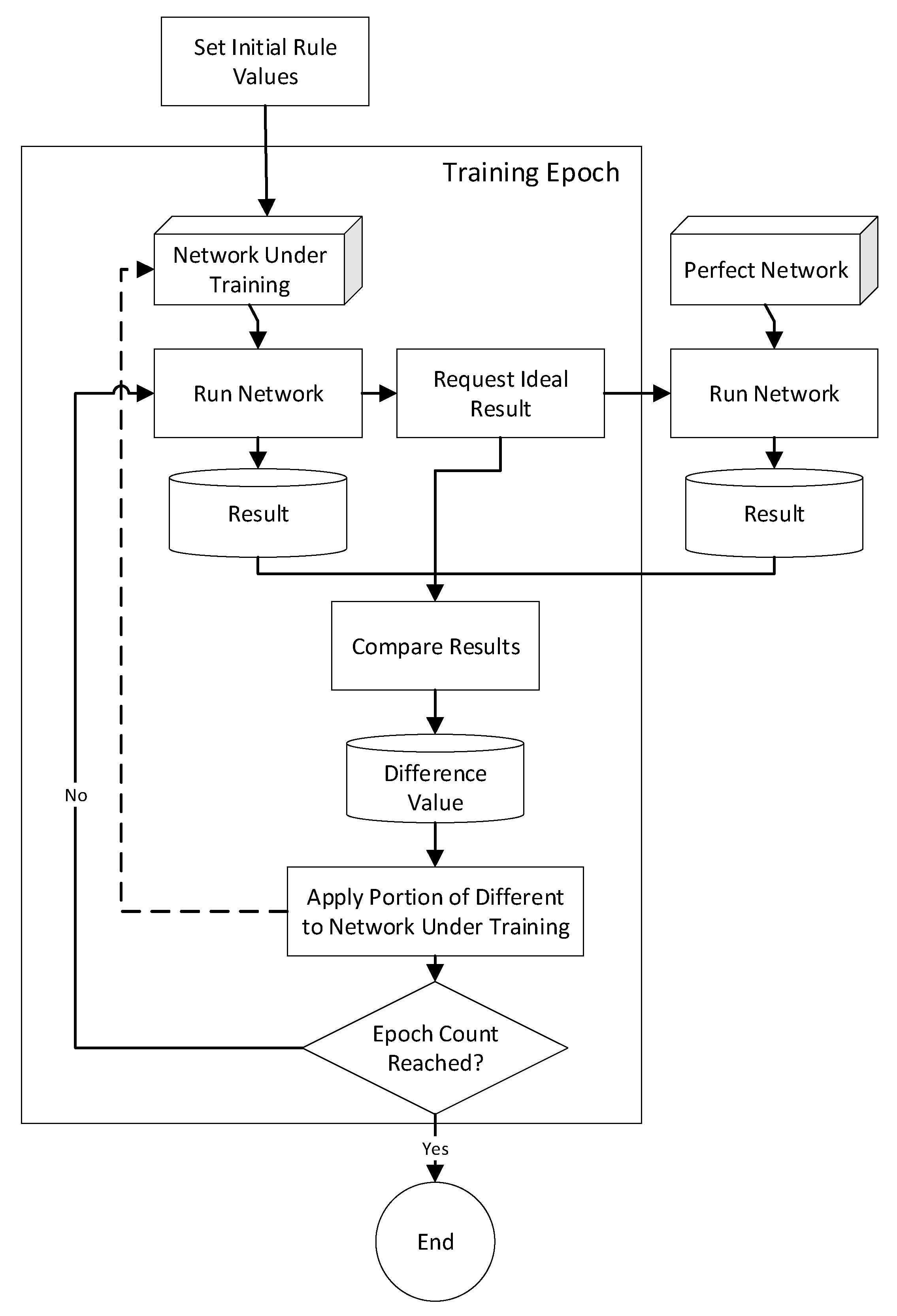
An approach, based on the identification of rules that directly or indirectly contribute to the target output fact, was proposed in [1] and is depicted in Figure 1 and Figure A1 (in Appendix A). Once the contributing rules are identified, a portion of the error between the target system-under-training’s output and the actual output, which is based on the rule’s level of contribution and a user-specified velocity value, is distributed to each contributing rule.
The training process, shown in Figure 1, starts with the network under training having initially set rule values (which are independent from the actual rule values of the perfect network, when using the perfect network testing approach presented in [35]) and its rule-fact network structure. The rule fact network structure that the network under training has is, excluding the random network case, based on the perfect network and may include network perturbations, based on the experimental condition being tested.
As part of the training process, both networks (the network under training and the perfect network) are run and the results of the two are compared to calculate a difference value, which is distributed to contributing rules using the algorithm depicted in Figure A1. The training process, which is described in more detail in Appendix A, is repeated for the user-specified number of training epochs.
In addition to the number epochs of training, the network configuration, the number of facts and rules, and the type of training used are also configurable. The four approaches to training used differ in the two ‘run network’ steps depicted in Figure 1. The approaches use different selection of initial and final rules for training.
The same-path techniques use the same initial and final node for all training while the multi-path techniques select a different starting and ending node for each training epoch. The same facts techniques utilize the same fact values, simulating an unchanging network, while the random facts techniques use different (randomly generated) facts to simulate a network with new data being collected for each training iteration. Note that the network weightings, which are what is being trained, are changed only by the training process. Because the network weightings of the ‘perfect’ network are applied to the fact data, phenomena-appropriate outputs (which are suitable for training use) are generated irrespective of whether the same or different fact values are used.
The training process and four training techniques are described in more detail in Appendix A. Section 3 describes the procedure that is used in Section 4, Section 5 and Section 6, where these parameters are used to define experimental conditions for this study.
2.4. Neural Networks and their Explainability Issues
The expert system rule-fact network training technique presented in Section 2.3 is responsive to key deficiencies of neural networks. These deficiencies and the explainable artificial intelligence (XAI) development effort that has developed in response to them are discussed in this section.
Neural networks have been shown to have issues with transparency, bias and the potential for learning non-causal relationships [36]. Many lack the ability to “explain their autonomous decisions to human users” [37] and some researchers have even suggested that there is an inverse relationship between system prediction quality and explainability [37]. Cyber-attackers have leveraged these weaknesses and neural networks’ lack of context knowledge to develop adversarial neural network attacks [38] against systems providing services such as voice [39] and facial recognition [40], among others. Neural network algorithms are among those identified by Doyle [41] as “weapons of math destruction” and by Noble [42] as “algorithms of oppression”.
XAI attempts to mitigate these problems by allowing human developers and users to understand how autonomous systems are making their decisions [37]. By advancing artificial intelligence from being “alchemy” within an opaque box, to a fully transparent “glass box” [43], it is thought that humans will be better able to assess whether systems are performing correctly and take appropriate actions. Arrieta, et al. [44] has suggested that XAI systems fall into two categories: there are techniques that provide a “degree of transparency” and others which are “interpretable to an extent by themselves”. Some techniques also exist to try to explain pre-existing opaque systems [44].
At present, XAI is a burgeoning area of work. XAI systems have been used for cyber intrusion [45] and fraud detection [46], lending [46], sales [46] and making recommendations [46], as well as mining and modeling [47] and command decision making for “small-unit tactical behavior” [48]. While XAI systems are a demonstrable advancement from opaque ones, Buhmann and Fieseler note that “simply the right to transparency will not create fairness” [49]. The defensible systems being studied in this paper seek to advance beyond XAI (while still being fully human understandable) to prevent—instead of just being able to explain and allow humans to prevent—erroneous decision making.
3. Experimental Design
This section discusses the experimental procedure and experimental system used for this work. First, the experimental system is discussed in Section 3.1. Then, in Section 3.2, the experimental procedure is presented.
3.1. Experimental System
The experimentation that is described in this paper was performed on a custom-implemented software application for developing and working with gradient descent trained expert system networks. This system has three key components. The first is a network module which performs all of the core functionality of the gradient descent trained expert system. It accepts commands to create the rule-fact network, stores the network, performs experimental network runs and implements the gradient descent training procedure.
The second is a network creation module. This module develops the random networks, based on specified parameters, which are used for experimentation. This module provides the network details to the first module which instantiates and stores these networks.
The third module is the experimental module. This module commands the testing. It starts individual test runs, collects run time data and collects the network output results to make them available for analysis.
This system was initially developed for the experimentation performed for [1].
3.2. Experimental Procedure
The procedure used for data collection in this study is based on the procedure used in [1] and is described in detail in [35]. The system is tested using a perfect network to provide inputs to the network that is being trained and tested under a given experimental condition. In [1], network size, network perturbation, training level and training velocity served as the independent variables that defined each experimental condition. For this study, network perturbation, training level and training velocity serve as the independent experimental condition-defining variables. Combinations of these variables are also used to define experimental conditions where the impact of different values for two or even all three concurrently are considered. In each section, and for each data table, the independent variables that are used to define the condition are identified. Table 1 presents a list of all possible parameter values.
For each experimental condition, which is defined by a selection of parameters from Table 1, 1000 runs were performed. For each run, a new randomly generated network was created, based on the parameters defining the experimental condition. In all cases, for this study, a 100-rule, 100-fact network was utilized. To make the network to be trained and evaluated, the perfect network was duplicated and the rule values reset. In cases where perturbation of the network is included, in the experimental condition definition, the newly created network would be altered, as indicated, before training commenced.
In some cases, generated networks would begin in a completed condition; in others, networks (due to their random construction) would not be completable. Networks which started completed or could not complete were excluded from the data presented in this study.
4. Network Types and System Performance
The assessment of the impact of different parameters on the two multi-path training techniques begins with consideration of the impact of network types on the techniques. Network impact bears consideration for two reasons. First, by assessing the performance of the training techniques under error and augmented networks, the robustness of the techniques to different levels of discrepancy between a phenomenon and its rule-fact network modeling is assessed. Second, networks could prospectively be altered to introduce augmentation or error, if this is found to be beneficial. The use of error and noise to aid training was briefly discussed in Section 2.2.
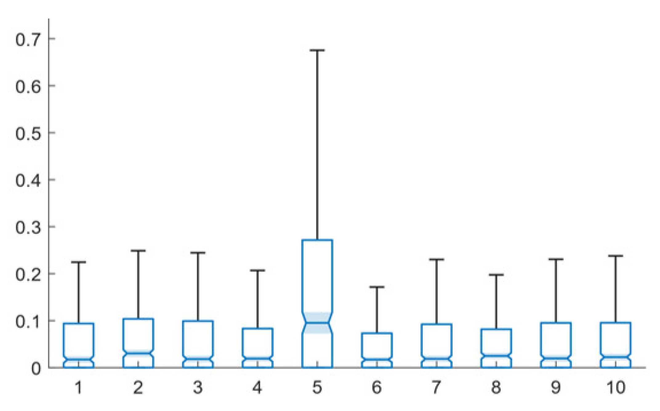
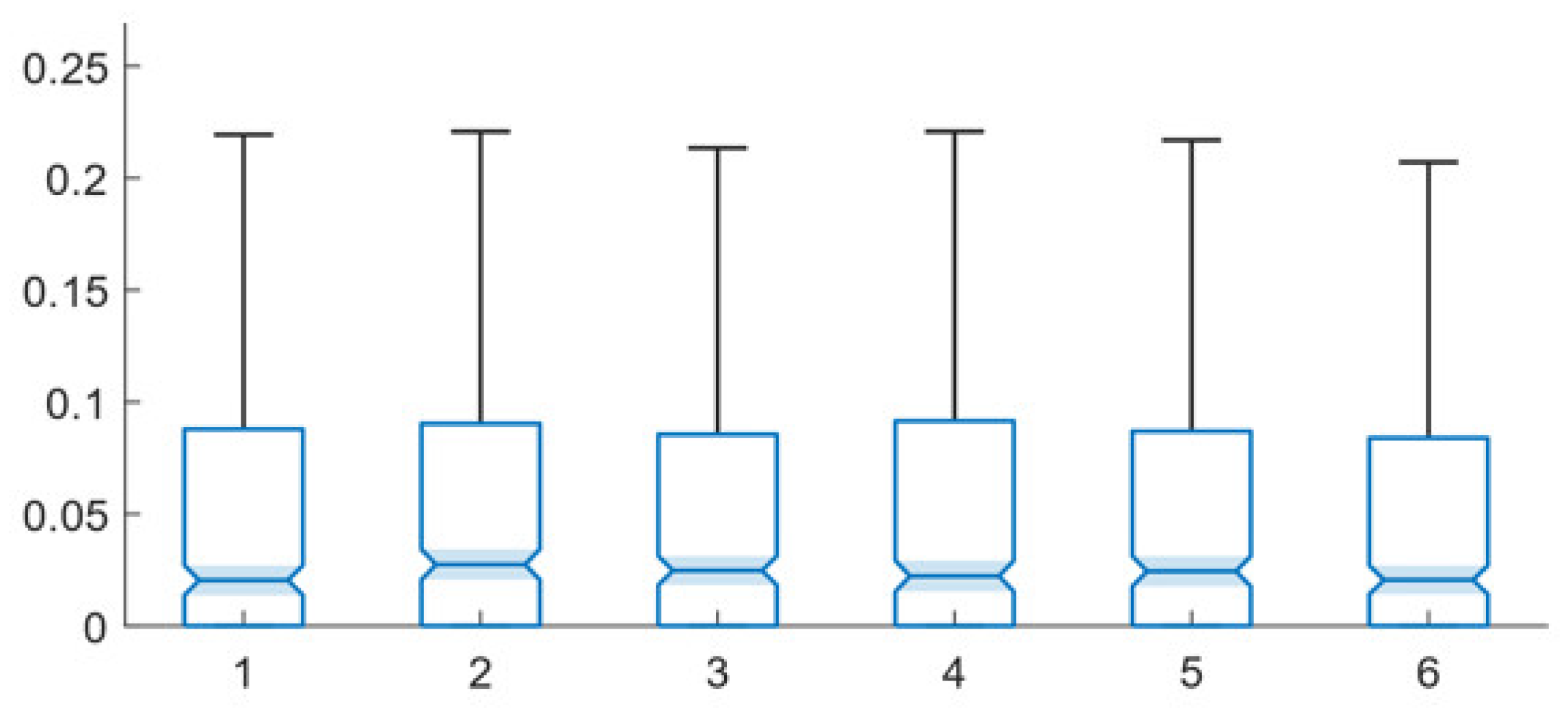
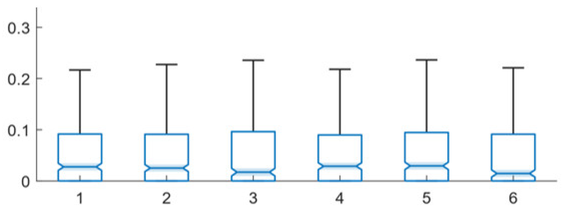
Figure 2 presents the performance of the multi-path, same facts training technique for different network-under-training network configurations and Figure 3 presents the performance of the multi-path, random facts training technique for different network configurations. The underlying data for these two figures is presented in Table A2 and Table A3 (in Appendix B), respectively.
Both techniques perform similarly for the base and the error-introduced and augmented networks. The lowest mean error level for both is actually generated by an augmented network (10% augmented for the multi-path, same facts technique and 1% augmented for the multi-path, random facts technique). The lowest median error level for the multi-path, same facts technique is also generated by the 10% augmented network, while the 1% augmented network and base network tie for performing best for the multi-path, random facts training technique, in terms of median error.
The random networks significantly underperform in all cases, except that random networks have the lowest mean value for the low-error networks for the multi-path, same facts technique; however, since random networks produce far less completions than other network types, this is not an indication of effective performance. Notably, both training approaches seem to not perform well with a small amount of error, as the 10% error networks are the second worst performing for both training types (random networks perform the worst for both mean and median error for both). However, for larger levels of error and augmentation, the mean and median error levels fluctuate between approximately 5.5% and 6%, with various configurations both outperforming and underperforming the base configuration.
The notched box plots in Figure 2 and Figure 3 show several statistically significant differences between the performances of different error and augmentation conditions. From this data, it is clear that the network structure is very important to the efficacy of gradient descent trained expert systems and to both multi-path training techniques. The nearly three-times greater error of the random network demonstrates this importance. However, it is also clear that both techniques are robust to small amounts of network error and augmentation. This is important, as it means that minor inaccuracies, omissions or additions in network design will not dramatically impact system performance. In fact, the results suggest that small levels of network augmentation, in particular, may even be slightly beneficial to system performance.
5. Training and System Performance
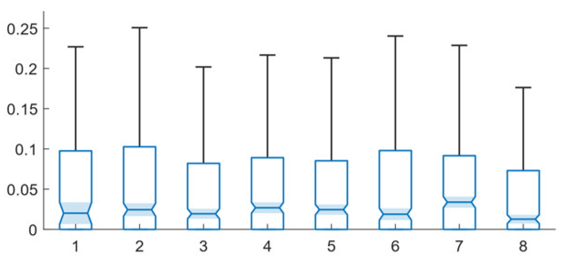
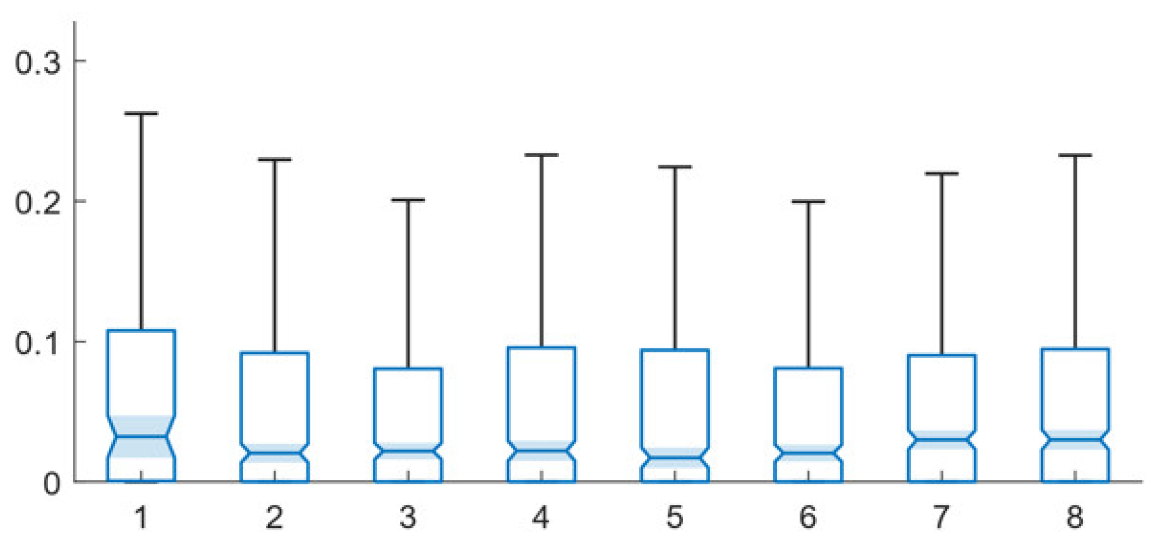
The assessment of the impact of different parameters on the two multi-path training techniques next considers the impact of different levels of training epochs on each training technique’s efficacy. Figure 4 and Figure 5 present data characterizing the performance of the multi-path, same facts and multi-path, random facts training techniques, respectively, with different levels of training epochs. The underlying data for these two figures is presented in Table A4 and Table A5 in Appendix B.
For the multi-path, same facts technique, the lowest mean error is produced by 1000 epochs of training. Given that the highest mean error is produced by 500 epochs of training, this is an ambiguous result. The second-best mean error is produced by 25 epochs of training. The use of 1000 epochs of training produces the lowest median error as well. Given the fluctuation present, it appears that there is no particular trend of more (or less) training enhancing network performance. This suggests that much of the efficacy of the system is produced by the rule-fact network, while at least a minimal amount of training is required.
A somewhat different result is apparent with the multi-path, random facts technique, from the data presented in Figure 5 and Table A5. The lowest mean error is produced by 25 training epochs and the lowest median error is produced by 100 training epochs. However, 250 training epochs underperforms 25 epochs, for mean error, by only 0.1%. Notably, at both the lowest and highest levels of training, the system has the lowest performance, in terms of mean error. A clear trend is present in both, with error dropping from 6.5% at one epoch of training to 5.4% at 10 epochs of training to 5.1% at 25 epochs of training and error rising from 5.2% at 250 epochs of training to 6.1% at 500 epochs of training to 6.5% at 1000 epochs of training. This suggests that the multi-path, random facts technique may benefit from additional training, up to a point, and may also suffer from over-training beyond a certain point. A similar, though less pronounced, trend is also present in the median error, which drops between the one and ten epochs training levels and rises between the 250 epochs and 500/1000 epochs training levels. Notably, when reviewing the notched box plots in Figure 4 and Figure 5, multiple statistically significant differences are present.
To assess whether different levels of training change system efficacy for different network configurations, Table 2 and Table 3 present data for evaluating the performance of the multi-path, same facts and multi-path, random facts training techniques, respectively, for different combinations of training epoch levels and network configuration.
For the multi-path, same facts technique, overall, the best performance, in terms of lowest mean error, is produced under the 25% error network with one training epoch. The base network, also with one training epoch, produces the best performance, in terms of the lowest median error.
For the base, 25% and 50% error networks, and the 25% augmented networks, one training epoch outperforms, in terms of both providing the lowest mean and median error levels (tying with 250 training epochs for the 25% augmented networks). For 10% augmented and random networks, the 100 epochs training level performs best, in terms of the lowest mean error level. For the 10% augmented networks, the lowest mean error is also produced by 100 epochs of training. The lowest median error value for the random networks was produced by 25 epochs of training. Given the foregoing, there are clear differences in the amount of training that is beneficial for different network types; however, overall less training seems to outperform additional training, suggesting that overtraining may be occurring, in at least some cases, at higher training epoch levels.
For the multi-path, random facts technique, the base network produces the best overall results. The lowest average mean value waws produced by one training epoch and the best median value was produced by 25 and 100 training epochs, all under the base network configuration.
Beyond this, the results are inconsistent across the different network types. The base and random networks have their lowest mean error with one training epoch. For the random networks, one training epoch also produces the lowest median error.
The 25-epoch level produces the best mean values for the 10% error, 25% error and 25% augmented networks (tying with 100 training epochs, in the case of the 25% error networks, and with 250 epochs, in the case of the 25% augmented networks). The 25 epoch training level also produces the lowest median error levels for the base (tying with 100 epochs) and 10% error networks. The 100-epoch training level produces the best results for the 25% error and 10% augmented networks, in terms of lowest mean error (tying with 250 epochs, in the case of the 10% augmented networks). The 100-epoch training level also produces the lowest mean value for the 25% error, 10% augmented and 25% augmented networks. Finally, the 250-epoch training level produces the best mean error level for both the 10% and 25% augmented networks (tying with 100 epochs, in the case of the 10% augmented networks). The 250-epoch training level also produces the lowest average median result for the 10% augmented networks (tying with the 100-epoch training level).
Given the foregoing, there is no clear level of training the works best, across the board, for all network types. Correlations between network type and training levels clearly exist. Practically, however, the implications of the differences between different levels of training may be limited. Excluding the random networks (which consistently have higher error levels), the range of average mean error values for each network type is between 0.5% and 1.1% and the range of average median values is between 0.5% and 1.4% across the different network types.
6. Velocity Levels and System Performance
In continuing the assessment of the impact of different parameters on the two multi-path training techniques, the impact of training velocity on the performance of the two techniques is now assessed. Figure 6 and Figure 7 present results that characterize the impact of velocity on system performance for the multi-path, same facts and multi-path random facts techniques, respectively. The underlying data for these comparisons is also presented in Table A6 and Table A7, in Appendix B.
For the multi-path, same facts technique, the base setting of a velocity of 0.01 outperforms other techniques in terms of the mean error level. The 0.5 setting outperforms in terms of the median error level.
The 0.5 velocity performs the best for the mean and median error levels for the multi-path, random facts training technique. Notably, this puts a significant amount of weight on the most recent training epochs. This is, interestingly, consistent with the multi-path, random facts performing well, in terms of median and mean of the low-error networks, at lower training levels, as discussed in Section 5 and shown in Table A5. Notably, no practical and statistically significant differences are present for the multi-path, same facts technique, while several statistically significant differences are present for the multi-path random facts technique.
The impact of different velocity levels on the performance of the multi-path, same facts and multi-path, random facts techniques for different network configurations is now considered. Data is presented in Table 4, Table 5, Table 6 and Table 7 for the two techniques comparing their performance with 0.01 and 0.25 velocity levels (Table A2 and Table A3 present data for the base 0.10 velocity level) for different network configurations.
The performance of the multi-path, same facts technique is somewhat similar between the three velocity levels for which data is presented in Table A2, Table 4 and Table 5. In each case the lowest mean error occurs under one of the augmented network types: for 0.01 velocity, it is in the 25% augmented networks, for 0.10 velocity, the best performance is with the 10% augmented networks and for velocity of 0.25, the best performance is also in the 10% augmented networks. For all three velocity levels, the lowest median error also occurred in these network types. Clearly, the training method is robust to all velocity settings across all network types.
In comparing the performance of the different velocities for each network type for the multi-path, same facts technique, the 0.25 velocity performs the best, outperforming others for the lowest mean error value for the base, 10% error, 25% error, 10% augmented and random networks. The 0.25 velocity performs best for the lowest median error for the 10% error, 10% augmented and random networks. The 0.01 velocity outperforms others for the lowest median error for the base networks and the 25% augmented networks for both the lowest mean error and lowest median error. The 0.10 velocity outperforms for the lowest median error for the 25% error networks.
For the multi-path, random facts training technique, the data in Table 6 and Table 7 shows that the technique is robust across all error and augmentation levels at all three velocity levels. The 25% error and 10% augmented networks produce the best performance, in terms of lowest mean error, at the 0.01 velocity level, while the 10% and 25% error networks produce the best performance, in terms of lowest mean error, at the 0.25 velocity level. In terms of lowest median error, the 25% augmented network produces the lowest error at the 0.01 velocity level and the 25% error produces the lowest median error at the 0.25 velocity level.
In comparing the performance of the different velocity values for each of the network types, the 0.01 velocity performs the strongest. It produces the lowest mean error values for the base, 25% error, 10% augmented and 25% augmented networks and the lowest median error for the 10% error, 10% augmented and 25% augmented networks. The 0.25 velocity setting performs best for both lowest mean and median error for the 10% error networks (tying with the 0.01 velocity’s median value). The 0.10 velocity outperforms in terms of lowest median error for the base and 25% error networks, and for both lowest mean and median error for the random networks.
The performance of the two techniques is now assessed for combinations of training epoch levels and velocity. Table 8 and Table 9 present this data for the 0.05 and 0.25 velocity levels. These can be compared to the data in Table A4 and Table A5 for the 0.10 velocity level.
For the multi-path, same facts technique, the best performance, in terms of lowest mean error, occurs with 1000 training epochs and 0.10 velocity. Not considering this data point, which is inconsistent with the data trends for the 0.10 velocity data, the 25 epochs and 0.10 velocity combination preforms best for lowest mean error. The lowest median error occurs at the 1000 training epoch level with 0.10 velocity.
Comparing the performance of the different training velocities for different levels of training epochs also shows the 0.10 velocity outperforming, in many cases. The 0.10 velocity performs the best for lowest median error for all training levels except for 100 epochs, where the 0.25 velocity outperforms by 0.1%, and, in terms of lowest mean error, for the 25 epochs training level. The 0.25 velocity performs best, in terms of mean error, for 1 and 100 training epochs and the 0.05 velocity performs best, in terms of mean error, for the 250 training epochs level. While there is no across-the-board best velocity or training epochs setting, smaller levels of training and mid-range velocity values appear to be, generally, outperforming other settings for the multi-path, same facts technique.
For the multi-path, random facts technique, the lowest mean error and lowest median error both were obtained from the 0.05 velocity with 1 epoch of training. The 0.05 velocity produced the lowest mean and median error levels for both 1 and 250 training epochs and the lowest mean for 100 epochs. The 0.10 velocity produced the lowest median error levels for the 25 and 100 training epoch levels and the lowest mean error for the 25 epochs training level. Like with the multi-path same facts technique, there is no across-the-board best velocity or training epochs setting; however, smaller levels of training and smaller velocity values appear to be, generally, outperforming larger ones for the multi-path, random facts technique.
Now, all four experimental condition parameters are considered together. For the multi-path, same facts networks, data in Table A2, Table 4, Table 5 and Table 10 is compared. For the multi-path, random facts networks, data in Table A3, Table 6, Table 7 and Table 11 is compared.
For the multi-path, same facts training technique, the best overall results are produced under the 10% augmented network using a velocity of 0.01 and 25 epochs of training. This condition produces both the lowest mean and lowest median error levels of any considered.
For the base network type, the best results were produced with a velocity of 0.01 and 25 epochs of training. For the 10% error networks, the lowest mean error was produced with a velocity of 0.25 and 100 epochs of training. The lowest median error was produced with a velocity of 0.1 and 25 epochs of training. For the 25% error networks, the lowest mean and median error were produced using a velocity of 0.25 and 25 epochs of training. For the 10% augmented networks, a velocity of 0.01 and 25 epochs of training produces both the lowest mean and median error levels. For the 25% augmented networks, the lowest mean and median error levels are produced using a velocity of 0.01 and 100 epochs of training. For the random networks, the lowest mean error is produced with a velocity of 0.01 and 25 epochs of training and the lowest median error level is produced using a velocity of 0.25 with 100 epochs of training. Given the foregoing, there is not a single technique that performs best across-the-board, though some seem to perform well more consistently than others.
For the multi-path, random facts technique, the best overall results are produced by the 1% augmented network, 100 training epochs and a velocity of 0.1, for lowest mean error, and 25 training epochs and a velocity of 0.01, for lowest median error.
For the base network, the lowest mean error was produced with 25 epochs of training and a velocity of 0.1 and the lowest median error was produced by both 25 epochs of training and a velocity of 0.01 and 100 epochs of training and a velocity of 0.1. For the 10% error networks, the lowest mean and median error levels are both produced with 25 epochs of training and a velocity of 0.1. For the 25% error networks, the lowest mean error value is produced by both a velocity of 0.01 and 100 epochs of training and a velocity of 0.01 and 25 epochs of training. The lowest median error is produced with 25 epochs of training and a velocity of 0.01.
For the 10% augmented networks, the lowest mean and median error levels are produced using a velocity of 0.01 and 100 epochs of training. For the 25% augmented networks, both the lowest mean and median error levels are produced using a velocity of 0.25 and 25 epochs of training. Finally, for the random networks, both the best mean and median error values are produced with a velocity of 0.01 and 25 epochs of training. While there is no single best set of settings, again lower velocity and lower training levels seem to be, generally, outperforming.
7. Comparative Performance of the Single-Path and Multi-Path Techniques
In [1], two multi-path techniques were introduced and the single- and multi-path techniques were briefly compared. Through this limited comparison, the multi-path techniques were shown to outperform the single-path techniques under the base (100 rules/100 facts, 100 training epochs, 0.1 velocity and non-perturbed network) configuration. However, further analysis was not conducted, in that study, on the multi-path techniques and their performance under other experimental conditions was not assessed. The single- and multi-path techniques were also not compared under any experimental conditions other than the base one.
Section 4, Section 5 and Section 6 have assessed the performance of the two multi-path techniques and compared the performance of the two techniques under different network perturbations, training epoch levels and with different training velocity settings. This section compares the performance of the multi-path techniques to the performance of the single path techniques, as presented in [1]. This analysis makes use of data presented in Table A2, Table A3, Table A4, Table A5, Table A6 and Table A7, and discussed previously in this article.
7.1. Network Perturbation
In comparing the single-path and multi-path techniques under networks with different perturbation levels, there are a number of similarities. Both multi-path techniques perform best, in terms of lowest mean error, with the augmented networks. The multi-path, random facts technique performs best with the 1% augmented networks. The multi-path, same facts technique performs best with the 10% augmented networks. The single-path, same facts technique performs best with the 10% error technique, in terms of lowest mean error; however, this performance is only 0.001 better than its performance with the 1% augmented technique.
Though the performance levels are quite similar (only 0.001 to 0.003 different), the single path, same facts technique performs best, in terms of median error, with the 25% error networks. The multi-path same facts technique performs best with the 10% augmented networks while the multi-path random facts technique performs best with the base and 1% augmented networks.
In addition to outperforming for the base experimental condition, both the multi-path techniques outperform the single path, same facts technique across all of the different error and augmentation levels, both in terms of mean error and median error values. The multi-path techniques perform up to nearly twice as well, in some instances, in terms of mean error and up to slightly over three times as well, in some instances, in terms of median error. Both multi-path techniques also outperform on the random networks. For mean error levels, they outperform by approximately 30%. For median error, they outperform by 70% and 110% for the multi-path, same facts and random facts techniques, respectively.
7.2. Training Epochs
The performance of the single path, same facts technique and multi-path same facts technique were quite similar across different training epoch levels. Both performed best, in terms of mean error, at 25 epochs (tied with 100 epochs in the case of the single path, same facts technique). Both also performed best, in terms of median error, at 1000 training epochs. The multi-path, same facts technique also had a tied best performance, in terms of median error, at 100 epochs.
The multi-path, random facts technique also had its best performance, in terms of mean error, at 25 training epochs. Its lowest median error levels occurred at 10 and 250 epochs, however.
Like with the analysis across different network perturbation configurations, both multi-path techniques outperformed the single-path, same facts technique at all levels of training in terms of both mean and median error. Notably, not only did they outperform when comparing each respective level, all training levels of both multi-path techniques outperformed the best performing level of the single-path, same facts technique.
7.3. Training Velocity Levels
The performance of the single-path, same facts and the multi-path techniques, again, had similar patterns—in this case, across different velocity levels. While the single-path, same facts technique had its best performance at a velocity of 0.15, the multi-path techniques performed the best at the levels of 0.01 and 0.5, in terms of mean error, for the same and random facts versions, respectively. The multi-path, same facts technique, the same-path, single facts technique and the multi-path, random facts technique performed best, in terms of median error, at 0.5 velocity.
Like with the performance under the different training epoch levels, both multi-path techniques outperformed the single-path, same facts technique at each respective level. Additionally, all velocity levels of both multi-path techniques outperformed the best performing level of the single path, same facts technique.
8. Algorithm Speed Assessment
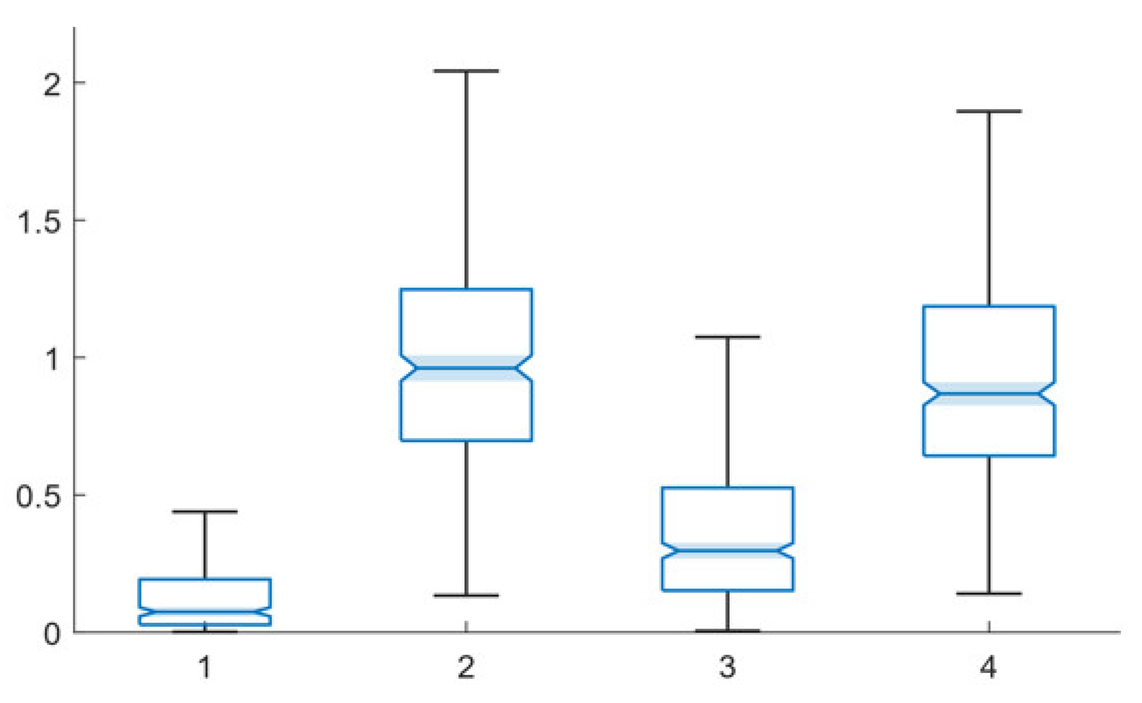
While accuracy is a key consideration, the computational cost of different training algorithms also needs to be considered. These costs are compared in this section. Table 12 presents the average training operating time for each of the four algorithms in units of timer ticks. Notably, the train path—same facts, the most basic technique, has the lowest computational cost. The train multiple paths—same facts technique has approximately double the cost of the train path—same facts techniques. Both of the random facts techniques are more computationally expensive. In both cases, the technique requires nearly 1,000,000 timer ticks to complete.
Figure 8 presents notched box plots for the training time data, demonstrating that the performance time differences are statistically significant in all cases. The computational speed is another key parameter into algorithm selection decision-making (along with accuracy level and data collection cost considerations). While the optimal selection will be driven by application needs, the comparatively high computational cost will serve as another factor in the train multiple paths—random facts technique not being preferred in most circumstances. The comparative computational costs of other techniques may be of limited concern in some applications (particularly where a network is trained once and used repeatedly); however, if training must be performed on a recurrent basis, for a time sensitive application or using limited computational capability hardware, this may not be the case.
9. Conclusions and Future Work
This paper has built on the work presented in [1] and assessed the performance of two multi-path techniques across a number of experimental conditions. Both techniques were shown to be robust to different network perturbations, training levels and training velocities. As would be expected, differences in performance were shown between different configurations and conditions; however, no catastrophic failure conditions or configurations were shown to exist, nor were any areas of comparatively exceptional performance identified. Unlike [1], this paper also analyzed combinations of two of the three independent variables and all three independent variables being varied together and showed that the multi-path techniques were robust to these configurations. Similar to the analysis of individual variable conditions, no catastrophic failure conditions or comparatively exceptional performance were identified from these multi-variable combination conditions. The techniques, thus, can be optimized for use in various applications based on the parameters of the particular application, informed by the data presented herein.
The techniques were also shown to consistently outperform the single-path, same facts technique evaluated in [1]. While the two multi-path techniques showed variation (in some cases correlating strongly with the variation of the single-path, same facts technique), no configurations where the same-path, same facts technique would outperform were identified. Given this, the multi-path techniques would be preferable to use, if ignoring the comparative cost of data collection. As the multi-path techniques utilize numerous input and output points across the network, this may drive a need for a larger scale of data collection and incur a correspondingly larger cost. This cost–benefit analysis is inherently an application specific consideration which is informed by the comparative performance comparison presented herein.
While the multi-path techniques consistently outperform the single-path, same facts technique, neither multi-path technique outperforms the other one across-the-board. In many cases, the difference between the performance of the two may be practically insignificant. Given this, there is minimal value to collecting the level of additional data that would be required to operate training of the multi-path, random facts style for a real-world application. While additional training data can be easily generated from a perfect network for simulation, in the real world the collection of this additional training data has an associated cost. Thus, for most applications, the multi-path, same facts approach will be a clear cost-benefit comparison winner as compared to the multi-path, random facts approach (which also has a higher computational cost, in addition to higher data collection costs). The data presented herein can inform this calculation for any given application area.
Overall, the data presented herein have demonstrated the efficacy of the multi-path techniques for use with the gradient descent trained expert system, initially presented in [1] and showed that the multi-path, same facts technique may be preferable for use for many applications. Future work will include the exploration of the techniques’ specific utility in various application areas as well as additional enhancements to and assessment of the gradient descent trained expert system concept. The assessment of other pre-existing optimization techniques (and gradient descent variants) to train rule-fact expert system networks and the development of new techniques for this purpose are also planned.
Funding
This research received no external funding.
Data Availability Statement
The author confirms that all relevant results data are included in the article. Underlying data is available from the author upon reasonable request.
Conflicts of Interest
The author declares no conflict of interest.
Appendix A. Gradient Descent Rule-Fact Network Training Technique
This appendix describes the gradient descent technique that was proposed in [1], which introduced gradient descent trained expert systems. The system is comprised of two parts: a classical forward-chaining expert system engine and the training module, which is now described, which optimizes the rule weightings within the expert system rule-fact network. In this system, each fact has a value between zero and one and rules have weighting values that define the contribution of each input facts to the output fact. Weighting values must be between zero and one and sum to one.
The system uses an approach that distributes a portion of the error, between the system-under-training’s output and the actual output, to rules which are identified as directly or indirectly contributing to the target output fact.
The training process, depicted in Figure 1 and outlined in pseudocode in Listing A1, starts with the network under training having rule values independent from the actual (perfect) network’s. However, the rule fact network structure that the network under training has, excluding the random network case, is based on the perfect network (possibly including network perturbations, for certain experimental conditions).
During training, the network under training and the perfect network are both run and the results of the two are used to calculate a difference value. The algorithm depicted in Figure A1 is used to distribute a portion of this, based on the velocity value and rule contributions, to the contributing rules. This training process is repeated for the user-specified number of training epochs.
The algorithm for determining the error-based difference value, shown in Figure A1, begins by identifying all nodes that impact the target fact directly. Then, all of the nodes that impact these nodes are iteratively identified and their indirect contributions are calculated. As each node is identified, it is added to the contributions list. The process of identifying and adding nodes is performed until no nodes are added during an iteration.
To determine the contribution of a rule, Ci in the equation below, to the target fact, the equation used is [1]:
The meaning of the different variables used in Equations (A1) and (A2) are listed in Table A1. If a rule is part of multiple rule-fact chains to the target fact, it may have multiple contribution values; however, only the highest value is retained and used for calculating its contribution.

Table A1.
Variable definitions for Equations (A1) and (A2).
| Variable | Meaning |
|---|---|
| Wi | Weighting for rule i |
| WR(m,h) | Weighting for each rule (m indicates the rule and h indicates which weight value) |
| {APT} | Set of all rules passed through |
| Ci | Contribution of rule i |
| {AC} | Set of all contributing rule nodes |
| RP | Perfect network result |
| RT | Training network result |
| V | Velocity |
| MAX | Function returning the largest value passed to it |
| Di | Difference applied to a given rule weighting |
To determine the difference value to be applied to a given rule weighting, Di, the contribution of the particular rule is divided by the total contribution of all rules, and multiplied by the velocity parameter and a value based on the difference between the expected and actual value for the given training run. This is computed by the equation:
Figure A1.
Node Change Determination Algorithm [1].
Figure A1.
Node Change Determination Algorithm [1].

One the level of change required to a node is determined, added or reduced weight is assigned to the higher and lower values’ input facts’ weightings.
The algorithm provides several parameters for customization. The velocity setting, as shown in Equation (A2), determines how much of the error-based difference value is applied and thus how responsive the network is to each training epoch. The number epochs of training, the network configuration, the number of facts and rules, and the type of training used are also configurable.
| Listing A1. Pseudocode for Algorithm. |
| Perfect Network Generation Using Relevant Parameters |
| { |
| Creation of Facts (including setting fact initial values) |
| Creation of Rules |
| Selection of Facts to Serve as Rule Inputs and Output |
| } |
| Creation of Network to be Trained |
| { |
| Copy rules and facts from perfect network |
| Apply network perturbations, if required for experimental condition |
| Reset all rule values |
| } |
| Training Process |
| { |
| For the specified number of training epochs |
| { |
| If training type = train path—same facts |
| { |
| Select input/output facts during first iteration, reuse throughout training |
| } |
| Elseif training type = train path—random facts |
| { |
| Select input/output facts during first iteration, reuse throughout training |
| Reset all fact values to new random values for the training epoch |
| } |
| Elseif training type = train multiple paths—same facts |
| { |
| Select input/output facts during each iteration |
| } |
| Elseif training type = train multiple paths—random facts |
| { |
| Select input/output facts during each iteration |
| Reset all fact values to new random values for the training epoch |
| } |
| Identify Contributing Rules |
| Run ideal network |
| Run network under training |
| Compare results of runs to determine error |
| Apply Part of Error Between Actual and Target Output to Contributing Rules |
| } |
| If fact values have been changed during training, reset to original values |
| } |
| Run Presentation Transaction to Collect Data |
Appendix B. Data Tables
This appendix presents data tables that support the notched box plot figures included in this paper. Table A2, Table A3, Table A4, Table A5, Table A6 and Table A7 provide supporting data for Figure 2, Figure 3, Figure 4, Figure 5, Figure 6 and Figure 7, respectively.
Table A2.
Error levels for multi-path, same facts training technique for base, error-present, augmented and random networks.
Table A2.
Error levels for multi-path, same facts training technique for base, error-present, augmented and random networks.
| Mean | Median | Mean—High Err | Mean—Low Err | |
|---|---|---|---|---|
| Base Network | 0.058 | 0.025 | 0.183 | 0.023 |
| 10% Error Network | 0.067 | 0.032 | 0.186 | 0.025 |
| 25% Error Network | 0.059 | 0.018 | 0.184 | 0.018 |
| 50% Error Network | 0.060 | 0.025 | 0.182 | 0.021 |
| Random Network | 0.178 | 0.118 | 0.322 | 0.016 |
| 1% Augmented Network | 0.057 | 0.021 | 0.176 | 0.022 |
| 5% Augmented Network | 0.053 | 0.022 | 0.174 | 0.022 |
| 10% Augmented Network | 0.051 | 0.017 | 0.170 | 0.022 |
| 25% Augmented Network | 0.059 | 0.031 | 0.175 | 0.025 |
| 50% Augmented Network | 0.053 | 0.020 | 0.162 | 0.020 |
Table A3.
Error levels for multi-path, random facts training technique for base, error-present, augmented and random networks.
Table A3.
Error levels for multi-path, random facts training technique for base, error-present, augmented and random networks.
| Mean | Median | Mean—High Err | Mean—Low Err | |
|---|---|---|---|---|
| Base Network | 0.059 | 0.017 | 0.190 | 0.019 |
| 10% Error Network | 0.065 | 0.030 | 0.177 | 0.024 |
| 25% Error Network | 0.054 | 0.018 | 0.161 | 0.019 |
| 50% Error Network | 0.054 | 0.019 | 0.182 | 0.021 |
| Random Network | 0.170 | 0.095 | 0.322 | 0.023 |
| 1% Augmented Network | 0.050 | 0.017 | 0.166 | 0.020 |
| 5% Augmented Network | 0.056 | 0.019 | 0.174 | 0.019 |
| 10% Augmented Network | 0.058 | 0.025 | 0.196 | 0.023 |
| 25% Augmented Network | 0.059 | 0.020 | 0.184 | 0.021 |
| 50% Augmented Network | 0.062 | 0.022 | 0.189 | 0.021 |
Table A4.
Error levels for multi-path, same facts training technique under different levels of training.
Table A4.
Error levels for multi-path, same facts training technique under different levels of training.
| Mean | Median | Mean—High Err | Mean—Low Err | |
|---|---|---|---|---|
| 1 Epoch | 0.059 | 0.020 | 0.184 | 0.020 |
| 10 Epochs | 0.062 | 0.024 | 0.180 | 0.020 |
| 25 Epochs | 0.054 | 0.019 | 0.180 | 0.022 |
| 50 Epochs | 0.056 | 0.027 | 0.167 | 0.025 |
| 100 Epochs | 0.058 | 0.025 | 0.183 | 0.023 |
| 250 Epochs | 0.057 | 0.019 | 0.172 | 0.019 |
| 500 Epochs | 0.063 | 0.034 | 0.188 | 0.025 |
| 1000 Epochs | 0.048 | 0.013 | 0.181 | 0.020 |
Table A5.
Error levels for multi-path, random facts training technique under different levels of training.
Table A5.
Error levels for multi-path, random facts training technique under different levels of training.
| Mean | Median | Mean—High Err | Mean—Low Err | |
|---|---|---|---|---|
| 1 Epoch | 0.065 | 0.032 | 0.180 | 0.026 |
| 10 Epochs | 0.054 | 0.021 | 0.170 | 0.021 |
| 25 Epochs | 0.051 | 0.022 | 0.171 | 0.024 |
| 50 Epochs | 0.057 | 0.022 | 0.175 | 0.021 |
| 100 Epochs | 0.059 | 0.017 | 0.190 | 0.019 |
| 250 Epochs | 0.052 | 0.021 | 0.170 | 0.022 |
| 500 Epochs | 0.061 | 0.030 | 0.184 | 0.023 |
| 1000 Epochs | 0.065 | 0.030 | 0.196 | 0.025 |
Table A6.
Error levels for multi-path, same facts training technique with different velocity levels.
Table A6.
Error levels for multi-path, same facts training technique with different velocity levels.
| Velocity | Mean | Median | Mean—High Err | Mean—Low Err |
|---|---|---|---|---|
| 0.01 | 0.057 | 0.021 | 0.183 | 0.022 |
| 0.05 | 0.060 | 0.027 | 0.187 | 0.023 |
| 0.1 | 0.058 | 0.025 | 0.183 | 0.023 |
| 0.15 | 0.059 | 0.022 | 0.181 | 0.021 |
| 0.25 | 0.056 | 0.024 | 0.176 | 0.021 |
| 0.5 | 0.056 | 0.020 | 0.180 | 0.021 |
Table A7.
Error levels for multi-path, random facts training technique with different velocity levels.
Table A7.
Error levels for multi-path, random facts training technique with different velocity levels.
| Velocity | Mean | Median | Mean—High Err | Mean—Low Err |
|---|---|---|---|---|
| 0.01 | 0.058 | 0.028 | 0.175 | 0.024 |
| 0.05 | 0.056 | 0.025 | 0.171 | 0.023 |
| 0.1 | 0.059 | 0.017 | 0.190 | 0.019 |
| 0.15 | 0.057 | 0.029 | 0.170 | 0.024 |
| 0.25 | 0.062 | 0.029 | 0.183 | 0.025 |
| 0.5 | 0.055 | 0.015 | 0.178 | 0.019 |
References
- Straub, J. Expert system gradient descent style training: Development of a defensible artificial intelligence technique. Knowl. Based Syst. 2021, 228, 107275. [Google Scholar] [CrossRef]
- Mitra, S.; Pal, S.K. Neuro-fuzzy expert systems: Relevance, features and methodologies. IETE J. Res. 1996, 42, 335–347. [Google Scholar] [CrossRef]
- Zwass, V. Expert System. Available online: https://www.britannica.com/technology/expert-system (accessed on 24 February 2021).
- Lindsay, R.K.; Buchanan, B.G.; Feigenbaum, E.A.; Lederberg, J. DENDRAL: A case study of the first expert system for scientific hypothesis formation. Artif. Intell. 1993, 61, 209–261. [Google Scholar] [CrossRef] [Green Version]
- Styvaktakis, E.; Bollen, M.H.J.; Gu, I.Y.H. Expert system for classification and analysis of power system events. IEEE Trans. Power Deliv. 2002, 17, 423–428. [Google Scholar] [CrossRef]
- McKinion, J.M.; Lemmon, H.E. Expert systems for agriculture. Comput. Electron. Agric. 1985, 1, 31–40. [Google Scholar] [CrossRef]
- Kuehn, M.; Estad, J.; Straub, J.; Stokke, T.; Kerlin, S. An expert system for the prediction of student performance in an initial computer science course. In Proceedings of the IEEE International Conference on Electro Information Technology, Lincoln, NE, USA, 14–17 May 2017. [Google Scholar]
- Kalogirou, S. Expert systems and GIS: An application of land suitability evaluation. Comput. Environ. Urban Syst. 2002, 26, 89–112. [Google Scholar] [CrossRef]
- Waterman, D. A Guide to Expert Systems; Addison-Wesley Pub. Co.: Reading, MA, USA, 1986. [Google Scholar]
- Renders, J.M.; Themlin, J.M. Optimization of Fuzzy Expert Systems Using Genetic Algorithms and Neural Networks. IEEE Trans. Fuzzy Syst. 1995, 3, 300–312. [Google Scholar] [CrossRef]
- Sahin, S.; Tolun, M.R.; Hassanpour, R. Hybrid expert systems: A survey of current approaches and applications. Expert Syst. Appl. 2012, 39, 4609–4617. [Google Scholar] [CrossRef]
- Zadeh, L.A. Fuzzy sets. Inf. Control 1965, 8, 338–353. [Google Scholar] [CrossRef] [Green Version]
- Chohra, A.; Farah, A.; Belloucif, M. Neuro-fuzzy expert system E_S_CO_V for the obstacle avoidance behavior of intelligent autonomous vehicles. Adv. Robot. 1997, 12, 629–649. [Google Scholar] [CrossRef]
- Sandham, W.A.; Hamilton, D.J.; Japp, A.; Patterson, K. Neural network and neuro-fuzzy systems for improving diabetes therapy. In Proceedings of the 20th Annual International Conference of the IEEE Engineering in Medicine and Biology Society, Hong Kong, China, 1 November 1998; Institute of Electrical and Electronics Engineers (IEEE): Picataway, NJ, USA, 2002; pp. 1438–1441. [Google Scholar]
- Ephzibah, E.P.; Sundarapandian, V. A Neuro Fuzzy Expert System for Heart Disease Diagnosis. Comput. Sci. Eng. Int. J. 2012, 2, 17–23. [Google Scholar] [CrossRef]
- Das, S.; Ghosh, P.K.; Kar, S. Hypertension diagnosis: A comparative study using fuzzy expert system and neuro fuzzy system. In Proceedings of the IEEE International Conference on Fuzzy Systems, Hyderabad, India, 7–10 July 2013. [Google Scholar]
- Akinnuwesi, B.A.; Uzoka, F.M.E.; Osamiluyi, A.O. Neuro-Fuzzy Expert System for evaluating the performance of Distributed Software System Architecture. Expert Syst. Appl. 2013, 40, 3313–3327. [Google Scholar] [CrossRef]
- Rojas, R. The Backpropagation Algorithm. In Neural Networks; Springer: Berlin/Heidelberg, Germany, 1996; pp. 149–182. [Google Scholar]
- Battiti, R. Accelerated Backpropagation Learning: Two Optimization Methods. Complex Syst. 1989, 3, 331–342. [Google Scholar]
- Kosko, B.; Audhkhasi, K.; Osoba, O. Noise can speed backpropagation learning and deep bidirectional pretraining. Neural Netw. 2020, 129, 359–384. [Google Scholar] [CrossRef] [PubMed]
- Abbass, H.A. Speeding Up Backpropagation Using Multiobjective Evolutionary Algorithms. Neural Comput. 2003, 15, 2705–2726. [Google Scholar] [CrossRef]
- Aicher, C.; Foti, N.J.; Fox, E.B. Adaptively Truncating Backpropagation Through Time to Control Gradient Bias. In Proceedings of the 35th Uncertainty in Artificial Intelligence Conference, Tel Aviv, Israel, 22–25 July 2019; pp. 799–808. [Google Scholar]
- Chizat, L.; Bach, F. Implicit Bias of Gradient Descent for Wide Two-layer Neural Networks Trained with the Logistic Loss. Proc. Mach. Learn. Res. 2020, 125, 1–34. [Google Scholar]
- Kolen, J.F.; Pollack, J.B. Backpropagation is Sensitive to Initial Conditions. Complex Syst. 1990, 4, 269–280. [Google Scholar]
- Zhao, P.; Chen, P.Y.; Wang, S.; Lin, X. Towards query-efficient black-box adversary with zeroth-order natural gradient descent. Proc. AAAI Conf. Artif. Intell. 2020, 34, 6909–6916. [Google Scholar] [CrossRef]
- Wu, Z.; Ling, Q.; Chen, T.; Giannakis, G.B. Federated Variance-Reduced Stochastic Gradient Descent with Robustness to Byzantine Attacks. IEEE Trans. Signal Process. 2020, 68, 4583–4596. [Google Scholar] [CrossRef]
- Saffaran, A.; Azadi Moghaddam, M.; Kolahan, F. Optimization of backpropagation neural network-based models in EDM process using particle swarm optimization and simulated annealing algorithms. J. Braz. Soc. Mech. Sci. Eng. 2020, 42, 73. [Google Scholar] [CrossRef]
- Gupta, J.N.D.; Sexton, R.S. Comparing backpropagation with a genetic algorithm for neural network training. Omega 1999, 27, 679–684. [Google Scholar] [CrossRef]
- Basterrech, S.; Mohammed, S.; Rubino, G.; Soliman, M. Levenberg—Marquardt training algorithms for random neural networks. Comput. J. 2011, 54, 125–135. [Google Scholar] [CrossRef]
- Kim, S.; Ko, B.C. Building deep random ferns without backpropagation. IEEE Access 2020, 8, 8533–8542. [Google Scholar] [CrossRef]
- Ma, W.D.K.; Lewis, J.P.; Kleijn, W.B. The HSIC bottleneck: Deep learning without back-propagation. In Proceedings of the AAAI Conference on Artificial Intelligence, New York, NY, USA, 7–12 February 2020; Volume 34, pp. 5085–5092. [Google Scholar]
- Park, S.; Suh, T. Speculative Backpropagation for CNN Parallel Training. IEEE Access 2020, 8, 215365–215374. [Google Scholar] [CrossRef]
- Lee, C.; Sarwar, S.S.; Panda, P.; Srinivasan, G.; Roy, K. Enabling Spike-Based Backpropagation for Training Deep Neural Network Architectures. Front. Neurosci. 2020, 14, 119. [Google Scholar] [CrossRef] [PubMed] [Green Version]
- Mirsadeghi, M.; Shalchian, M.; Kheradpisheh, S.R.; Masquelier, T. STiDi-BP: Spike time displacement based error backpropagation in multilayer spiking neural networks. Neurocomputing 2021, 427, 131–140. [Google Scholar] [CrossRef]
- Straub, J. Machine learning performance validation and training using a ‘perfect’ expert system. MethodsX 2021, 8, 101477. [Google Scholar] [CrossRef]
- Li, J.; Huang, J.S. Dimensions of artificial intelligence anxiety based on the integrated fear acquisition theory. Technol. Soc. 2020, 63, 101410. [Google Scholar] [CrossRef]
- Gunning, D.; Stefik, M.; Choi, J.; Miller, T.; Stumpf, S.; Yang, G.Z. XAI-Explainable artificial intelligence. Sci. Robot. 2019, 4, eaay7120. [Google Scholar] [CrossRef] [Green Version]
- Eykholt, K.; Evtimov, I.; Fernandes, E.; Li, B.; Rahmati, A.; Xiao, C.; Prakash, A.; Kohno, T.; Song, D. Robust Physical-World Attacks on Deep Learning Models. arXiv 2017, arXiv:1707.08945. [Google Scholar]
- Gong, Y.; Poellabauer, C. Crafting Adversarial Examples for Speech Paralinguistics Applications. arXiv 2017, arXiv:1711.03280v2. [Google Scholar] [CrossRef]
- Sharif, M.; Bhagavatula, S.; Bauer, L.; Reiter, M.K. Accessorize to a Crime: Real and Stealthy Attacks on State-of-the-Art Face Recognition. In Proceedings of the 2016 ACM SIGSAC Conference on Computer and Communications Security, Vienna, Austria, 24–28 October 2016; ACM Press: New York, NY, USA, 2016; pp. 1528–1540. [Google Scholar]
- Doyle, T. Weapons of Math Destruction: How Big Data Increases Inequality and Threatens Democracy. Inf. Soc. 2017, 33, 301–302. [Google Scholar] [CrossRef]
- Noble, S.U. Algorithms of Oppression: How Search Engines Reinforce Racism Paperback; NYU Press: New York, NY, USA, 2018. [Google Scholar]
- Xu, F.; Uszkoreit, H.; Du, Y.; Fan, W.; Zhao, D.; Zhu, J. Explainable AI: A Brief Survey on History, Research Areas, Approaches and Challenges. In Proceedings of the CCF International Conference on Natural Language Processing and Chinese Computing 2019, Dunhuang, China, 9−14 October 2019. [Google Scholar]
- Barredo Arrieta, A.; Díaz-Rodríguez, N.; Del Ser, J.; Bennetot, A.; Tabik, S.; Barbado, A.; Garcia, S.; Gil-Lopez, S.; Molina, D.; Benjamins, R.; et al. Explainable Explainable Artificial Intelligence (XAI): Concepts, taxonomies, opportunities and challenges toward responsible AI. Inf. Fusion 2020, 58, 82–115. [Google Scholar] [CrossRef] [Green Version]
- Mahbooba, B.; Timilsina, M.; Sahal, R.; Serrano, M. Explainable Artificial Intelligence (XAI) to Enhance Trust Management in Intrusion Detection Systems Using Decision Tree Model. Complexity 2021, 2021, 1–11. [Google Scholar] [CrossRef]
- Gade, K.; Geyik, S.C.; Kenthapadi, K.; Mithal, V.; Taly, A. Explainable AI in Industry. In Proceedings of the 25th ACM SIGKDD International Conference on Knowledge Discovery & Data Mining, Anchorage, AK, USA, 4–8 August 2019. [Google Scholar]
- Mehdiyev, N.; Fettke, P. Explainable Artificial Intelligence for Process Mining: A General Overview and Application of a Novel Local Explanation Approach for Predictive Process Monitoring. arXiv 2020, arXiv:2009.02098. [Google Scholar]
- Van Lent, M.; Fisher, W.; Mancuso, M. An explainable artificial intelligence system for small-unit tactical behavior. In Proceedings of the 16th Conference on Innovative Applications of Artificial Intelligence, San Jose, CA, USA, 27–29 July 2004. [Google Scholar]
- Buhmann, A.; Fieseler, C. Towards a deliberative framework for responsible innovation in artificial intelligence. Technol. Soc. 2021, 64, 101475. [Google Scholar] [CrossRef]
Figure 1.
Training Process [1].
Figure 1.
Training Process [1].

Figure 2.
Error level box plots for multi-path, same facts training technique for base, error-present, augmented and random networks: 1—base, 2—10% error, 3—25% error, 4—50% error, 5—random, 6—1% augmented, 7—5% augmented, 8—10% augmented, 9—25% augmented, 10—50% augmented.
Figure 2.
Error level box plots for multi-path, same facts training technique for base, error-present, augmented and random networks: 1—base, 2—10% error, 3—25% error, 4—50% error, 5—random, 6—1% augmented, 7—5% augmented, 8—10% augmented, 9—25% augmented, 10—50% augmented.

Figure 3.
Error levels for multi-path, random facts training technique for base, error-present, augmented and random networks: 1—base, 2—10% error, 3—25% error, 4—50% error, 5—random, 6—1% augmented, 7—5% augmented, 8—10% augmented, 9—25% augmented, 10—50% augmented.
Figure 3.
Error levels for multi-path, random facts training technique for base, error-present, augmented and random networks: 1—base, 2—10% error, 3—25% error, 4—50% error, 5—random, 6—1% augmented, 7—5% augmented, 8—10% augmented, 9—25% augmented, 10—50% augmented.

Figure 4.
Error levels for multi-path, same facts training technique under different levels of training: 1—base, 2—10% error, 3—25% error, 4—50% error, 5—random, 6—1% augmented, 7—5% augmented, 8—10% augmented, 9—25% augmented, 10—50% augmented.
Figure 4.
Error levels for multi-path, same facts training technique under different levels of training: 1—base, 2—10% error, 3—25% error, 4—50% error, 5—random, 6—1% augmented, 7—5% augmented, 8—10% augmented, 9—25% augmented, 10—50% augmented.

Figure 5.
Error levels for multi-path, random facts training technique under different levels of Table 1. 1—base, 2—10% error, 3—25% error, 4—50% error, 5—random, 6—1% augmented, 7—5% augmented, 8—10% augmented, 9—25% augmented, 10—50% augmented.
Figure 5.
Error levels for multi-path, random facts training technique under different levels of Table 1. 1—base, 2—10% error, 3—25% error, 4—50% error, 5—random, 6—1% augmented, 7—5% augmented, 8—10% augmented, 9—25% augmented, 10—50% augmented.

Figure 6.
Error levels for multi-path, same facts training technique with different velocity levels: 1—base, 2—10% error, 3—25% error, 4—50% error, 5—random, 6—1% augmented, 7—5% augmented, 8—10% augmented, 9—25% augmented, 10—50% augmented.
Figure 6.
Error levels for multi-path, same facts training technique with different velocity levels: 1—base, 2—10% error, 3—25% error, 4—50% error, 5—random, 6—1% augmented, 7—5% augmented, 8—10% augmented, 9—25% augmented, 10—50% augmented.

Figure 7.
Error levels for multi-path, random facts training technique with different velocity levels: 1—base, 2—10% error, 3—25% error, 4—50% error, 5—random, 6—1% augmented, 7—5% augmented, 8—10% augmented, 9—25% augmented, 10—50% augmented.
Figure 7.
Error levels for multi-path, random facts training technique with different velocity levels: 1—base, 2—10% error, 3—25% error, 4—50% error, 5—random, 6—1% augmented, 7—5% augmented, 8—10% augmented, 9—25% augmented, 10—50% augmented.

Figure 8.
Notched box plot comparison of speed performance of the training techniques (scale values are on ×106 scale): 1—train path—same facts, 2—train path—random facts, 3—train multiple paths—same facts, 4—train multiple paths—random facts.
Figure 8.
Notched box plot comparison of speed performance of the training techniques (scale values are on ×106 scale): 1—train path—same facts, 2—train path—random facts, 3—train multiple paths—same facts, 4—train multiple paths—random facts.

Table 1.
Experimental hyperparameters.
| Model Hyperparameters | Experimental Parameters | Algorithm Hyperparameters | |||
|---|---|---|---|---|---|
| Facts | Rules | Network Perturbation | Training Epochs | Velocity | Training Approach |
| 100 | 100 | Base Random Augmented 1% Augmented 5% Augmented 10% Augmented 25% Augmented 50% Error 10% Error 25% Error 50% | 1 10 25 50 100 250 500 1000 | 0.01 0.05 0.10 0.15 0.25 0.50 | Multiple Paths—Same Facts Multiple Paths—Random Facts |
Table 2.
Error levels for multi-path, same facts training technique for base, error-present, augmented and random networks under different levels of training.
Table 2.
Error levels for multi-path, same facts training technique for base, error-present, augmented and random networks under different levels of training.
| Network | Training | Mean | Median | Mean—High Err | Mean—Low Err |
|---|---|---|---|---|---|
| Base | 1 | 0.051 | 0.010 | 0.204 | 0.018 |
| 25 | 0.061 | 0.023 | 0.197 | 0.023 | |
| 100 | 0.058 | 0.025 | 0.183 | 0.023 | |
| 250 | 0.057 | 0.023 | 0.176 | 0.023 | |
| 10% Error | 1 | 0.051 | 0.017 | 0.168 | 0.017 |
| 25 | 0.057 | 0.019 | 0.179 | 0.020 | |
| 100 | 0.067 | 0.032 | 0.186 | 0.025 | |
| 250 | 0.049 | 0.018 | 0.165 | 0.022 | |
| 25% Error | 1 | 0.048 | 0.017 | 0.165 | 0.020 |
| 25 | 0.058 | 0.029 | 0.175 | 0.026 | |
| 100 | 0.059 | 0.018 | 0.184 | 0.018 | |
| 250 | 0.057 | 0.025 | 0.175 | 0.023 | |
| 10% Augmented | 1 | 0.060 | 0.030 | 0.184 | 0.024 |
| 25 | 0.050 | 0.021 | 0.165 | 0.021 | |
| 100 | 0.051 | 0.017 | 0.170 | 0.022 | |
| 250 | 0.057 | 0.023 | 0.179 | 0.021 | |
| 25% Augmented | 1 | 0.058 | 0.021 | 0.168 | 0.018 |
| 25 | 0.061 | 0.032 | 0.177 | 0.025 | |
| 100 | 0.059 | 0.031 | 0.175 | 0.025 | |
| 250 | 0.058 | 0.027 | 0.171 | 0.023 | |
| Random | 1 | 0.191 | 0.161 | 0.293 | 0.019 |
| 25 | 0.182 | 0.111 | 0.341 | 0.015 | |
| 100 | 0.178 | 0.118 | 0.322 | 0.016 | |
| 250 | 0.197 | 0.148 | 0.342 | 0.016 |
Table 3.
Error levels for multi-path, random facts training technique for base, error-present, augmented and random networks under different levels of training.
Table 3.
Error levels for multi-path, random facts training technique for base, error-present, augmented and random networks under different levels of training.
| Network | Training | Mean | Median | Mean—High Err | Mean—Low Err |
|---|---|---|---|---|---|
| Base | 1 | 0.052 | 0.031 | 0.162 | 0.027 |
| 25 | 0.058 | 0.017 | 0.190 | 0.020 | |
| 100 | 0.059 | 0.017 | 0.190 | 0.019 | |
| 250 | 0.057 | 0.021 | 0.179 | 0.021 | |
| 10% Error | 1 | 0.059 | 0.025 | 0.165 | 0.019 |
| 25 | 0.054 | 0.021 | 0.186 | 0.023 | |
| 100 | 0.065 | 0.030 | 0.177 | 0.024 | |
| 250 | 0.064 | 0.029 | 0.193 | 0.024 | |
| 25% Error | 1 | 0.059 | 0.022 | 0.179 | 0.019 |
| 25 | 0.054 | 0.023 | 0.169 | 0.022 | |
| 100 | 0.054 | 0.018 | 0.161 | 0.019 | |
| 250 | 0.056 | 0.021 | 0.175 | 0.024 | |
| 10% Augmented | 1 | 0.063 | 0.019 | 0.193 | 0.017 |
| 25 | 0.062 | 0.027 | 0.181 | 0.022 | |
| 100 | 0.058 | 0.025 | 0.196 | 0.023 | |
| 250 | 0.058 | 0.025 | 0.178 | 0.024 | |
| 25% Augmented | 1 | 0.058 | 0.031 | 0.172 | 0.025 |
| 25 | 0.054 | 0.021 | 0.167 | 0.023 | |
| 100 | 0.059 | 0.020 | 0.184 | 0.021 | |
| 250 | 0.054 | 0.021 | 0.179 | 0.023 | |
| Random | 1 | 0.152 | 0.067 | 0.317 | 0.016 |
| 25 | 0.181 | 0.105 | 0.335 | 0.019 | |
| 100 | 0.170 | 0.095 | 0.322 | 0.023 | |
| 250 | 0.191 | 0.138 | 0.343 | 0.013 |
Table 4.
Error levels for multi-path, same facts training technique for base, error-present, augmented and random networks with a 0.01 velocity level.
Table 4.
Error levels for multi-path, same facts training technique for base, error-present, augmented and random networks with a 0.01 velocity level.
| Network | Velocity | Mean | Median | Mean—High Err | Mean—Low Err |
|---|---|---|---|---|---|
| Base | 0.01 | 0.057 | 0.021 | 0.183 | 0.022 |
| 10% Error | 0.01 | 0.060 | 0.026 | 0.177 | 0.022 |
| 25% Error | 0.01 | 0.066 | 0.029 | 0.186 | 0.023 |
| 10% Augmented | 0.01 | 0.055 | 0.019 | 0.195 | 0.021 |
| 25% Augmented | 0.01 | 0.053 | 0.020 | 0.170 | 0.021 |
| Random | 0.01 | 0.188 | 0.129 | 0.336 | 0.014 |
Table 5.
Error levels for multi-path, same facts training technique for base, error-present, augmented and random networks with a 0.25 velocity level.
Table 5.
Error levels for multi-path, same facts training technique for base, error-present, augmented and random networks with a 0.25 velocity level.
| Network | Velocity | Mean | Median | Mean—High Err | Mean—Low Err |
|---|---|---|---|---|---|
| Base | 0.25 | 0.056 | 0.024 | 0.176 | 0.021 |
| 10% Error | 0.25 | 0.053 | 0.020 | 0.185 | 0.023 |
| 25% Error | 0.25 | 0.057 | 0.019 | 0.195 | 0.020 |
| 10% Augmented | 0.25 | 0.050 | 0.015 | 0.175 | 0.021 |
| 25% Augmented | 0.25 | 0.055 | 0.023 | 0.178 | 0.023 |
| Random | 0.25 | 0.175 | 0.106 | 0.334 | 0.013 |
Table 6.
Error levels for multi-path, random facts training technique for base, error-present, augmented and random networks with a 0.01 velocity level.
Table 6.
Error levels for multi-path, random facts training technique for base, error-present, augmented and random networks with a 0.01 velocity level.
| Training | Velocity | Mean | Median | Mean—High Err | Mean—Low Err |
|---|---|---|---|---|---|
| Base | 0.01 | 0.058 | 0.028 | 0.175 | 0.024 |
| 10% Error | 0.01 | 0.061 | 0.025 | 0.189 | 0.022 |
| 25% Error | 0.01 | 0.053 | 0.027 | 0.164 | 0.023 |
| 10% Augmented | 0.01 | 0.053 | 0.020 | 0.173 | 0.020 |
| 25% Augmented | 0.01 | 0.057 | 0.019 | 0.177 | 0.020 |
| Random | 0.01 | 0.185 | 0.132 | 0.328 | 0.020 |
Table 7.
Error levels for multi-path, random facts training technique for base, error-present, augmented and random networks with a 0.25 velocity level.
Table 7.
Error levels for multi-path, random facts training technique for base, error-present, augmented and random networks with a 0.25 velocity level.
| Training | Velocity | Mean | Median | Mean—High Err | Mean—Low Err |
|---|---|---|---|---|---|
| Base | 0.25 | 0.062 | 0.029 | 0.183 | 0.025 |
| 10% Error | 0.25 | 0.057 | 0.025 | 0.178 | 0.025 |
| 25% Error | 0.25 | 0.057 | 0.023 | 0.178 | 0.023 |
| 10% Augmented | 0.25 | 0.063 | 0.028 | 0.194 | 0.023 |
| 25% Augmented | 0.25 | 0.059 | 0.024 | 0.174 | 0.024 |
| Random | 0.25 | 0.187 | 0.130 | 0.332 | 0.015 |
Table 8.
Error levels for multi-path, same facts training technique for different training levels with 0.05 and 0.25 velocity levels.
Table 8.
Error levels for multi-path, same facts training technique for different training levels with 0.05 and 0.25 velocity levels.
| Training | Velocity | Mean | Median | Mean—High Err | Mean—Low Err |
|---|---|---|---|---|---|
| 1 | 0.05 | 0.057 | 0.030 | 0.189 | 0.025 |
| 1 | 0.25 | 0.056 | 0.022 | 0.156 | 0.022 |
| 25 | 0.05 | 0.060 | 0.021 | 0.188 | 0.022 |
| 25 | 0.25 | 0.057 | 0.024 | 0.171 | 0.022 |
| 100 | 0.05 | 0.060 | 0.027 | 0.187 | 0.023 |
| 100 | 0.25 | 0.056 | 0.024 | 0.176 | 0.021 |
| 250 | 0.05 | 0.056 | 0.026 | 0.174 | 0.024 |
| 250 | 0.25 | 0.058 | 0.023 | 0.186 | 0.022 |
Table 9.
Error levels for multi-path, random facts training technique for different training levels with 0.05 and 0.25 velocity levels.
Table 9.
Error levels for multi-path, random facts training technique for different training levels with 0.05 and 0.25 velocity levels.
| Training | Velocity | Mean | Median | Mean—High Err | Mean—Low Err |
|---|---|---|---|---|---|
| 1 | 0.05 | 0.046 | 0.014 | 0.163 | 0.025 |
| 1 | 0.25 | 0.057 | 0.021 | 0.157 | 0.016 |
| 25 | 0.05 | 0.060 | 0.025 | 0.175 | 0.024 |
| 25 | 0.25 | 0.057 | 0.023 | 0.171 | 0.022 |
| 100 | 0.05 | 0.056 | 0.025 | 0.171 | 0.023 |
| 100 | 0.25 | 0.062 | 0.029 | 0.183 | 0.025 |
| 250 | 0.05 | 0.051 | 0.016 | 0.181 | 0.020 |
| 250 | 0.25 | 0.059 | 0.023 | 0.188 | 0.022 |
Table 10.
Error levels for multi-path, same facts training technique for base, error-present, augmented and random networks with different velocity levels and 25 epochs of training.
Table 10.
Error levels for multi-path, same facts training technique for base, error-present, augmented and random networks with different velocity levels and 25 epochs of training.
| Training | Network | Velocity | Mean | Median | Mean—High Err | Mean—Low Err |
|---|---|---|---|---|---|---|
| 25 Epoch | Base | 0.01 | 0.055 | 0.020 | 0.177 | 0.021 |
| 25 Epoch | Base | 0.1 | 0.061 | 0.023 | 0.197 | 0.023 |
| 25 Epoch | Base | 0.25 | 0.060 | 0.025 | 0.184 | 0.022 |
| 25 Epoch | 10% Error | 0.01 | 0.059 | 0.026 | 0.180 | 0.024 |
| 25 Epoch | 10% Error | 0.1 | 0.057 | 0.019 | 0.179 | 0.020 |
| 25 Epoch | 10% Error | 0.25 | 0.061 | 0.026 | 0.177 | 0.024 |
| 25 Epoch | 25% Error | 0.01 | 0.058 | 0.023 | 0.190 | 0.023 |
| 25 Epoch | 25% Error | 0.1 | 0.058 | 0.029 | 0.175 | 0.026 |
| 25 Epoch | 25% Error | 0.25 | 0.048 | 0.006 | 0.189 | 0.017 |
| 25 Epoch | 10% Augmented | 0.01 | 0.046 | 0.013 | 0.164 | 0.020 |
| 25 Epoch | 10% Augmented | 0.1 | 0.050 | 0.021 | 0.165 | 0.021 |
| 25 Epoch | 10% Augmented | 0.25 | 0.061 | 0.025 | 0.183 | 0.023 |
| 25 Epoch | 25% Augmented | 0.01 | 0.059 | 0.026 | 0.185 | 0.023 |
| 25 Epoch | 25% Augmented | 0.1 | 0.061 | 0.032 | 0.177 | 0.025 |
| 25 Epoch | 25% Augmented | 0.25 | 0.055 | 0.024 | 0.181 | 0.024 |
| 25 Epoch | Random | 0.01 | 0.173 | 0.135 | 0.315 | 0.016 |
| 25 Epoch | Random | 0.1 | 0.182 | 0.111 | 0.341 | 0.015 |
| 25 Epoch | Random | 0.25 | 0.186 | 0.121 | 0.331 | 0.015 |
Table 11.
Error levels for multi-path, random facts training technique for base, error-present, augmented and random networks with different velocity levels and 25 epochs of training.
Table 11.
Error levels for multi-path, random facts training technique for base, error-present, augmented and random networks with different velocity levels and 25 epochs of training.
| Training | Network | Velocity | Mean | Median | Mea—High Err | Mean—Low Err |
|---|---|---|---|---|---|---|
| 25 Epoch | Base | 0.01 | 0.055 | 0.021 | 0.172 | 0.023 |
| 25 Epoch | Base | 0.1 | 0.058 | 0.017 | 0.190 | 0.020 |
| 25 Epoch | Base | 0.25 | 0.066 | 0.030 | 0.185 | 0.024 |
| 25 Epoch | 10% Error | 0.01 | 0.057 | 0.024 | 0.183 | 0.021 |
| 25 Epoch | 10% Error | 0.1 | 0.054 | 0.021 | 0.186 | 0.023 |
| 25 Epoch | 10% Error | 0.25 | 0.062 | 0.026 | 0.179 | 0.022 |
| 25 Epoch | 25% Error | 0.01 | 0.053 | 0.014 | 0.180 | 0.018 |
| 25 Epoch | 25% Error | 0.1 | 0.054 | 0.023 | 0.169 | 0.022 |
| 25 Epoch | 25% Error | 0.25 | 0.056 | 0.022 | 0.173 | 0.022 |
| 25 Epoch | 10% Augmented | 0.01 | 0.057 | 0.024 | 0.182 | 0.022 |
| 25 Epoch | 10% Augmented | 0.1 | 0.062 | 0.027 | 0.181 | 0.022 |
| 25 Epoch | 10% Augmented | 0.25 | 0.059 | 0.026 | 0.178 | 0.023 |
| 25 Epoch | 25% Augmented | 0.01 | 0.058 | 0.021 | 0.189 | 0.021 |
| 25 Epoch | 25% Augmented | 0.1 | 0.054 | 0.021 | 0.167 | 0.023 |
| 25 Epoch | 25% Augmented | 0.25 | 0.055 | 0.017 | 0.170 | 0.019 |
| 25 Epoch | Random | 0.01 | 0.156 | 0.076 | 0.315 | 0.015 |
| 25 Epoch | Random | 0.1 | 0.181 | 0.105 | 0.335 | 0.019 |
| 25 Epoch | Random | 0.25 | 0.184 | 0.117 | 0.330 | 0.016 |
Table 12.
Comparison of the performance of the different training techniques.
| Training Technique | Average Time |
|---|---|
| Train Path—Same Facts | 170,921.0 |
| Train Path—Random Facts | 995,436.0 |
| Train Multiple Paths—Same Facts | 376,210.8 |
| Train Multiple Paths—Random Facts | 925,475.3 |
Publisher’s Note: MDPI stays neutral with regard to jurisdictional claims in published maps and institutional affiliations. |
© 2021 by the author. Licensee MDPI, Basel, Switzerland. This article is an open access article distributed under the terms and conditions of the Creative Commons Attribution (CC BY) license (https://creativecommons.org/licenses/by/4.0/).
Share and Cite
MDPI and ACS Style
Straub, J. Assessment of Gradient Descent Trained Rule-Fact Network Expert System Multi-Path Training Technique Performance. Computers 2021, 10, 103. https://0-doi-org.brum.beds.ac.uk/10.3390/computers10080103
AMA Style
Straub J. Assessment of Gradient Descent Trained Rule-Fact Network Expert System Multi-Path Training Technique Performance. Computers. 2021; 10(8):103. https://0-doi-org.brum.beds.ac.uk/10.3390/computers10080103
Chicago/Turabian StyleStraub, Jeremy. 2021. "Assessment of Gradient Descent Trained Rule-Fact Network Expert System Multi-Path Training Technique Performance" Computers 10, no. 8: 103. https://0-doi-org.brum.beds.ac.uk/10.3390/computers10080103
Note that from the first issue of 2016, this journal uses article numbers instead of page numbers. See further details here.