Application of the Hurricane-Based Optimization Algorithm to the Phase-Balancing Problem in Three-Phase Asymmetric Networks

Abstract

This article addresses the problem of optimal phase-swapping in asymmetric distribution grids through the application of hurricane-based optimization algorithm (HOA). The exact mixed-integer nonlinear programming (MINLP) model is solved by using a master–slave optimization procedure. The master stage is entrusted with the definition of load connection at each stage by using an integer codification that ensures that, per node, only one from the possible six-load connections is assigned. In the slave stage, the load connection set provided by the master stage is applied with the backward/forward power flow method in its matricial form to determine the amount of grid power losses. The computational performance of the HOA was tested in three literature test feeders composed of 8, 25, and 37 nodes. Numerical results show the effectiveness of the proposed master–slave optimization approach when compared with the classical Chu and Beasley genetic algorithm (CBGA) and the discrete vortex search algorithm (DVSA). The reductions reached with HOA were $24.34\%$, $4.16\%$, and $19.25\%$ for the 8-, 28-, and 37-bus systems; this confirms the literature reports in the first two test feeders and improves the best current solution of the IEEE 37-bus grid. All simulations are carried out in the MATLAB programming environment.

1. Introduction

1.1. General Context

Distribution systems have developed in an exponential growth due to the progress of society with its multiple application purposes and technological developments, which are focused on meeting the vital or material needs of human beings [1,2]. However, this growth generates problems in different distribution systems associated with load unbalance, which is caused by the impossibility of anticipating the input performance and the increase in end-users in the various nodes of the system. Considering that the type of connection of most loads is single-phase, it is relatively more economical (compared to a three-phase system) to build primary circuits (of a main three-phase section) with derivations of one or two phases toward sectors with less load [3,4].

This performance causes undesired scenarios [5] such as an increase in current in certain phases of the system, the appearance of current flow in the neutral conductor, overvoltages in the less loaded stages, increased power losses, economic penalties for the network operators, low economic efficiency in the electrical distribution system, inadequate operation of protections, and deterioration of the quality indexes in the distribution system [6].

In order to minimize power losses in distribution systems, different alternatives have been evaluated to mitigate the problem. One of these methods consists of the implementation of reactive compensation systems [7]; unfortunately, their acquisition generates high costs. Another alternative uses distributed generators; however, their main applications are for the reduction in greenhouse gas emissions or energy purchasing cost minimization, as their maintenance and operating costs are too expensive to be recovered only with energy loss minimization. A different option with a wide range of studies on it is the phase balance obtained through computational optimization; this resource, in comparison to its predecessors, does not require significant investments or disturb the stability of the network [8].

1.2. Motivation

By applying the hurricane-based optimization algorithm (HOA) for phase balancing in distribution systems, we, as authors, seek to minimize the active power losses of the system, because this optimization alternative generates appropriate voltage profiles for the system studied [5]. Avoiding monetary penalties was established by the Regulatory Commission for Power and Gas (CREG, its Spanish abbreviation), which provides the network code 025 of 1995. This code is the main instrument in terms of reliability corresponding to the general administrative provisions that establish the criteria for efficiency, quality, reliability, safety, continuity, and sustainability. Here, it establishes the limits of voltage profiles that cannot exceed an uncertainty of +/− 10% (and in terms of frequency, an uncertainty level of 3% of the nominal operating frequency of the system) [9]. On the other hand, it favors grid operators’ power purchase costs and consequently benefits the end-user in terms of associated costs.

1.3. Review of the State of the Art

In the development of distribution systems, there has been an emerging need to optimize each process that makes up the energy supply [10]; likewise, the need to reduce power losses was a starting point to develop different methods and algorithms, some of them created for phase balancing utilizing phase reorganization. This method was introduced in 1998 by [11], and it consisted of mixed-integer programming with linear constraints for phase balancing, which minimizes the unbalance of currents in the lines of distribution systems. In 1999, employing a simulated annealing metaheuristic algorithm, advances were made in the phase balancing development, with which total operating costs were minimized [12].

In the 2000s, phase balancing development using a genetic algorithm was proposed. This algorithm seeks to reduce stage unbalance in the proposed system  [13]. It was not until 2004 that the phase-swapping method was developed by applying a genetic algorithm addressed for distribution systems [14]. Subsequently, in 2005, a heuristic search algorithm with backward recurrence was used for phase-balance development, which reduced the neutral current [15]. The same year experienced an advance in an algorithm called ant colony optimization, which was aimed at distribution systems and managed to minimize phase unbalance within 24 h [16]. In 2006, a new optimization algorithm called particle swarm for phase balancing was published; this algorithm, in addition to reducing active power losses, also improved the voltage profiles of the system [17].

In 2008, algorithms were developed further to reduce system operating costs. Two such algorithms were developed, an expert system based on heuristic rules [18] and an immune algorithm that optimized costs in less than 24 h [19]. Two years later, phase balancing was performed employing automatic phase shifting, which consisted of obtaining the power flow and mapping it from the system information, thus determining the best phase configuration to achieve the lowest loss reduction [20]. By using load-flow equations linked to current and voltage constraints that balance the current flowing through the phases and likewise in the neutral cable of the system, two algorithms were developed: one in 2011, which was a fuzzy hybrid greedy heuristic algorithm [21], and another a self-adaptive hybrid differential evolution algorithm designed in 2012 [22]. A new algorithm was developed in 2012 based on bacterial foraging oriented by a particle swarm optimization algorithm. This phase-balancing algorithm minimizes the system operating costs regardless of its configuration (radial or meshed) [23].

In 2012, an algorithm that sought to minimize energy losses in distribution systems was developed, which generated a notorious reduction in the congestion of the distribution lines [8]. In 2016, the base balance was formulated utilizing two algorithms. The first one used a heuristic method based on phase exchange, which reduced system imbalance [24]. The second one was based on the verification of each system node, thus searching for the possible combination to perform the optimal phase exchange as long as it balanced the system [25]. Another algorithm aiming at phase unbalance based on the particle swarm optimization method was developed in 2018 [26]. This same year, it was proposed to minimize the imbalance in distribution systems employing a heuristic search algorithm that generated an optimal system phase shift using contactors for the loads [27]. A year later, it was implemented in coding based on group theory to minimize power losses in distribution systems through a genetic algorithm [28]. Other algorithms aiming at minimizing power losses have been developed to date, such as the analytical approach algorithms, which perform a minimum base exchange [29]. There is a similar algorithm with the purpose of optimization in a 24 h interval [30].

With the aforementioned revision of the state of the art regarding the phase-swapping problem, it has been demonstrated that there are multiple optimization algorithms applicable to phase balancing. Regardless of the method used, these techniques seek to increase the power quality and energy quality of distribution systems, offering benefits for network operators by reducing their energy purchase from the generating actors of the Colombian power system. Therefore, a meta-heuristic technique, the HOA, directed for phase balancing will be carried out; this application has not been developed yet. Likewise, the objective function of this implementation will be the minimization of active power losses in distribution systems.

1.4. Contributions

An in-depth study has been carried out to determine the feasibility of this proposed method as an optimal solution to phase balancing in distribution systems, detailing a master–slave optimization, which works as follows: Master phase: The arrangement system to be evaluated with its respective set of connections is determined [3]. Slave phase: Employing the three-phase iterative sweep method, it is a solution to the power flow and, specifically, the power losses in the system under study is determined [6], corresponding to the set of connections described in the master phase. HOA is applied to determine the number of possible connections and their location in space, thus obtaining the best connection set selection for the studied system.

By investigating the application of the algorithm based on hurricane behavior in distribution systems, it is possible to obtain development in uncharted spaces for the phase balance solution. Throughout sensitivity analysis between the number of possible solutions and the number of plots located in the study space to apply the algorithm based on hurricanes, it becomes feasible to select the best point to consider the hurricane center, thus deciding the set of optimized connections for the system phase balancing [6].

A computational code has been developed, which is capable of being applied in radial or meshed network topology without a limit of defined solution connections considering any number of nodes (note: in the computational validations, only radial grids will be used since these are the most common topologies reported in the current literature). The execution time of this computational code has been reduced using encoded integer variables that decrease the number of binary vectors in the application of the algorithm based on hurricanes and the use of an approximate master–slave optimization. Throughout this study, we demonstrate the effectiveness, facility, and fast solution to the unbalance of phases in three-phase distribution systems by comparing its efficiency with computational codes of the Chu and Beasley genetic algorithm (CBGA) [3] and the discrete vortex search algorithm (DVSA) [5].

1.5. Document Organization

This paper is structured in the following order: Section 2 presents the mixed-integer nonlinear programming (MINLP) model that represents the problem of the optimal phase-swapping in unbalanced distribution networks. Section 3 specifies the master–slave method, coupling the algorithm about hurricane performance and the matricial backward/forward power flow method. Section 4 presents scenarios from the specialized literature with their main electrical characteristics and subsequent evaluation. Section 5 demonstrates the numerical validation and comparison of results using the MATLAB software showing the values obtained and the reduction in power losses in distribution systems. Finally, Section 6 presents the conclusions obtained in this article.

2. Mathematical Model

The optimal phase-swapping problem at each node of unbalanced distribution systems must be represented with an MINLP model [6,31]. The objective function determines the sum of losses in all phases. In the first instance, the decision variables are reflected in the integer variables, which resemble the existing connection types for each system load. However, the parameters for this formulation are obtained from the characteristics of the distribution system. Due to the power flow equations and interactions between the voltage magnitudes at each node, the system is considered nonlinear in nature  [32,33]. Its purpose depends on the optimal selection of the load connection group that allows the system to find an operating point that reduces the studied phase disequilibrium.

2.1. Objective Function

The objective function applied in this study corresponds to Equation (1), which concerns the minimization of total grid losses during peak load consumption [6]:

$$minZ=\sum _{\gamma \in \mathsf{\Lambda }}\sum _{\lambda \in \mathsf{\Lambda }}\sum _{i\in \mathsf{\Psi }}\sum _{j\in \mathsf{\Psi }}{V}_i^{\gamma }{V}_j^{\lambda }{Y}_{ij}^{\lambda \gamma }cos\left({\delta }_i^{\gamma }-{\delta }_j^{\lambda }-{\theta }_{ij}^{\lambda \gamma }\right)$$

(1)

where Z represents the minimum value of the function. The sets inscribed to the phase and node systems, respectively, are $\mathsf{\Lambda }$ and $\mathsf{\Psi }$. $\lambda$ corresponds to the phases for nodes i and j, which identify the buses of the system. The magnitudes of voltages correspond to $V_i^{\gamma }$ and $V_j^{\lambda }$ with their respective angles ${\delta }_i^{\gamma }$ and ${\delta }_j^{\lambda }$, respectively. $Y_{ij}^{\lambda \gamma }$ is the magnitude of the admittances associated with the line connected between nodes i and j for the phases $\lambda$ and $\gamma$, respectively, with their respective angle ${\theta }_{ij}^{\lambda \gamma }$.

2.2. Constraints

To represent the system of the active power balance equilibrium at each node, we use Equation (2) as presented in [34]:

$$\begin{array}{c}\hfill P_i^{s\lambda }-\sum _{\lambda \in \mathsf{\Lambda }}{X}_{i\lambda \gamma }{P}_i^{d\lambda }=\sum _{\gamma \in \mathsf{\Lambda }}\sum _{j\in \mathsf{\Psi }}{V}_i^{\lambda }{Y}_{ij}^{\lambda \gamma }{V}_j^{\gamma }cos\left({\delta }_i^{\lambda }-{\delta }_j^{\gamma }-{\theta }_{ij}^{\lambda \gamma }\right),\left\{\forall \lambda \in \mathsf{\Lambda },\forall i\in \mathsf{\Psi }\right\}\end{array}$$

(2)

where the active power delivered by the slack node s of the system for each phase $\lambda$ is presented as $P_i^{s\lambda }$ at each node i. This is performed in such a manner that active power $P_i^{d\lambda }$ represents the power consumed by the system in phase $\lambda$ and for each node i; therefore, the decision variable $X_{i\lambda \gamma }$ is of a binary type; it selects among the possible joints for the loads associated with the demand.

Note that for the group of individuals $X_{i\lambda \gamma }$, there are six possible connections combining the sequence of phases in each load per node (see

Table 1. Possible load connections per phase in a particular node of the network.

Connection Group	Connection	Sequence	Variable ${\mathit{X}}_{\mathit{i}\mathit{\lambda }\mathit{\gamma }},\left\{\mathit{\lambda }=\{\mathit{a},\mathit{b},\mathit{c}\},\mathit{\gamma }=\{\mathit{a},\mathit{b},\mathit{c}\}\right\}$
1	ABC		$\left[\begin{array}{ccc}1& 0& 0\\ 0& 1& 0\\ 0& 0& 1\end{array}\right]$
2	BCA	Unchanged	$\left[\begin{array}{ccc}0& 1& 0\\ 0& 0& 1\\ 1& 0& 0\end{array}\right]$
3	CAB		$\left[\begin{array}{ccc}0& 0& 1\\ 1& 0& 0\\ 0& 1& 0\end{array}\right]$
4	ACB		$\left[\begin{array}{ccc}1& 0& 0\\ 0& 0& 1\\ 0& 1& 0\end{array}\right]$
5	CBA	Changed	$\left[\begin{array}{ccc}0& 0& 1\\ 0& 1& 0\\ 1& 0& 0\end{array}\right]$
6	BAC		$\left[\begin{array}{ccc}0& 1& 0\\ 1& 0& 0\\ 0& 0& 1\end{array}\right]$

). In the case that the distribution system contains induction machines in some nodes of the network, it is important to ensure that the sequence of the voltages remains constant to avoid damage in these machines [8].

The limitation with purely inductive loads (motors) in the system changing its configuration could affect its operation, producing associated deteriorations [35].

Additionally, six connection types are observed. The first one is the original connection without any variation. The following ones correspond to connection variations with possible sequence changes.

Figure 1 shows the possible change of connection selected by the algorithm, starting from a connection ABC to a connection BAC with a sequence change.

If the system does not have the three phases connected, we take their values as zero in the missing phase or phases [5].

To represent the reactive power equilibrium at each node i per phase, we use Equation (3) as defined in [34]:

$$\begin{array}{c}\hfill Q_i^{s\lambda }-\sum _{\lambda \in \mathsf{\Lambda }}{X}_{i\lambda \gamma }{Q}_i^{d\lambda }=\sum _{\gamma \in \mathsf{\Lambda }}\sum _{j\in \mathsf{\Psi }}{V}_i^{\lambda }{Y}_{ij}^{\lambda \gamma }{V}_j^{\gamma }sin\left({\delta }_i^{\lambda }-{\delta }_j^{\gamma }-{\theta }_{ij}^{\lambda \gamma }\right),\left\{\forall \lambda \in \mathsf{\Lambda },\forall i\in \mathsf{\Psi }\right\}\end{array}$$

(3)

where the reactive power delivered by the slack node s of the system for each phase $\lambda$ is presented as $Q_i^{s\lambda }$ at each node i, respectively. The reactive power $Q_i^{d\lambda }$ represents the power consumed by the system in each phase $\lambda$ at each bus i.

Inequality constraint (4) specifies the voltage regulation restrictions per phase at each node [36].

$$V_{min}\le V_i^{\lambda }\le V_{max},\left\{\forall i\in \mathsf{\Psi },\forall \lambda \in \mathsf{\Lambda }\right\}$$

(4)

Note that, for the voltage regulation restrictions, we are taking values between the maximum potential $V_{max}$ and minimum $V_{min}$ for each phase $\lambda$ at node i.

Since this study aims to obtain a single optimal connection for the system, it uses the constraints shown in Equations (5) and (6) [37].

$$\begin{array}{c}\hfill \sum _{\lambda \in \mathsf{\Lambda }}{X}_{i\lambda \gamma }=1,\left\{\forall i\in \mathsf{\Psi },\forall \gamma \in \mathsf{\Lambda }\right\}\end{array}$$

(5)

$$\begin{array}{c}\hfill \sum _{\gamma \in \mathsf{\Lambda }}{X}_{i\lambda \gamma }=1,\left\{\forall i\in \mathsf{\Psi },\forall \lambda \in \mathsf{\Lambda }\right\}\end{array}$$

(6)

The solution for the model described above requires a numerical optimization technique because its active and reactive power equations are neither convex nonlinear in nature [5]. Therefore, a master–slave method is proposed to solve its optimal phase balance using the HOA and the iterative sweep method in three-phase distribution systems.

Remark  1.

The main characteristic of the proposed optimization model (1) to (6) associated with the power balance equations defined in (2) and (3) is that these are only applicable to star connected loads, because in the case of the loads connected in a triangle, it is not possible to uncouple the phase-to-phase demand as a phase-to-neutral load. However, the presented model is used only to illustrate the complexity of the phase-swapping problem in distribution networks.

3. Solution Methodology

For the solution of a distribution system optimization case, based on minimizing the active power losses, taking into account a constant demand and using the master–slave structure, the HOA is in the master stage; the slave stage corresponds to the iterative three-phase flow [6]. Below is an explanation of the proposed stages.

3.1. Master Stage: HOA

Since this algorithm is a nonlinear method and binary in nature, it can be solved by using a meta-heuristic approach [38]. This technique is nature-inspired and mainly based on the observation of radial wind and pressure profiles. In this technique, the meteorological performance is described as the change of temperature over the Earth’s surface, where regions of low and high pressures originate corresponding to the geographical location. Therefore, this pressure difference provides atmospheric gases or winds, which flow from the high-pressure region to the low-pressure region. Subsequently, tropical and subtropical seas receive large amounts of energy from the sun, where it is transferred to the atmosphere in the form of water vapor, generating the movement of air perpendicular to the Earth and creating a low-pressure zone; here, the rotation in the direction of the earth’s rotation is established, containing the energy of this spiral airflow known as a hurricane. In summary, the hurricane is a low-pressure zone with a warm core that forms over the tropical and subtropical oceans, highlighting its three main parts: the eye (the center of the hurricane, low-pressure zone), the eyewall (area of high and deep clouds in the form of a ring, registering the most intense surrounding winds), and the rain bands (area of excessive rainfall in a spiral shape converging toward the center).

3.1.1. Initial Population

The HOA method requires an initial population, which is constituted by the wind plots. In the algorithm, these wind plots are represented by the nodes of the system. In this manner, validation is made possible for each possible solution [39]. The matrix size is determined by the number of plots required and the search space; each individual in the matrix is randomly established within the search space [38]. The form of the initial population is presented in Equation (7):

$$\mathbf{X}=\left[\begin{array}{ccccc}{x}_1^1& x_2^1& x_3^1& \cdots & x_i^1\\ x_1^2& x_2^2& x_3^2& \cdots & x_i^2\\ ⋮& ⋮& ⋮& \ddots & ⋮\\ x_1^n& x_2^n& x_3^n& \cdots & x_i^n\end{array}\right]$$

(7)

where matrix $\mathbf{X}$ corresponds to the initial population, and $x_i^n$ represents the possible connection of node i and the n solution group. Additionally, Equation (8) represents random numbers with uniform distribution, which are used to generate all population members [6]:

$$x_i^n=\mathrm{floor}\left(x_{min}+(x_{max}-x_{min})·\mathrm{rand}\left(1\right)\right)$$

(8)

where rand(1) is a random number between 0 and 1 with uniform distribution; floor () takes the integer part of the argument; and $x_{min}$ and $x_{max}$ are the minimum and maximum values that variable x can take, which for the phase-swapping problem is as recommended in [6], and they are defined as 1 and 7, respectively. It is relevant to mention that the initial population contains the best solution and initial position of the eye of the hurricane.

3.1.2. Displacement Wind Plots

Concerning their basic physical structure, winds initially increase exponentially toward the center then rapidly decay to quiescence. In contrast, the pressure decreases exponentially toward the center and settles in the low-pressure zone within the eye of the hurricane, and this forms a belt of intense winds known as the maximum radius of the surrounding wind ($R_{max}$), where the maximum radius is modified in a manner that it increases from the initial radius [40].

According to this performance, the vortex formed on the hurricane’s horizontal surface top is approximated by a logarithmic spiral pattern, where each pattern $x_i^n$ is a new location for each plot from its previous position; following the path of the spiral from a specific time t, this is described in Equations (9) and (10) [41].

$$x_i^n\left(t\right)=r_i\left(t\right)+e_i$$

(9)

$$r_i\left(t\right)=R_0{\exp }^{\left(\mathrm{rand}\left(1\right)·{\phi }_i\left(t\right)\right)}$$

(10)

Equation (9) shows that $r_i$ is the radius of the hurricane in its polar expression. The rational numbers $e_i$ are the coordinates of the hurricane eye or the spiral center and correspond to the best option obtained from the set of solutions mentioned in detail below in Section 3.1.3. In the case of Equation (10), $R_0$ and $\mathrm{rand}\left(\right)$ are the variables that determine the spiral shape. Then, it is evident that $\mathrm{rand}\left(\right)$ contained in the exponential indicates the spiral increase rate and, together with its sign, determines the spiral rotation direction, while $R_0$ indicates the initial hurricane eye. Under initial conditions, when time $t=0$, ${\phi }_i\left(0\right)$ is, therefore, proceeds to zero; consequently, $r_i$ is equal to the initial radius, i.e., $R_0$, which is a user-defined positive number [38].

The possible solutions or plots need velocity to initiate and maintain motion. Therefore, velocity in the method is considered to be an angular change rate. The next angular coordinate $\phi \left(t\right)$ presents the velocity increase to the previous angular coordinate $\phi (t-1)$ [40]. The algorithm links the basic hurricane shape and the historical work on general whirlpools related to logarithmic spirals. Therefore, the combinatorial-Rankine presented by Depperman is the most appropriate model for this technique [38]; this model is a simple parametric description of two equations of a swirling flow. Similarly, the inner radial region around the center of the flow is a solid rotation. In contrast, the outer sector is vorticity-free as observed in Equation (11).

$${\phi }_i\left(t\right)=\left\{\begin{array}{ccc}\phi \left(t\right)+\omega ,& \mathrm{if}& r_i\le R_{max}\\ \phi \left(t\right)+\omega ·{\left(\frac{R_{max}}{r}\right)}^{\mathrm{rand}\left(1\right)},& \mathrm{if}& r_i>R_{max}\end{array}\right.$$

(11)

Regarding the radial region between the center of the hurricane and $R_{max}$, it must maintain its angular momentum due to the laws of physics, meaning that the angular velocity is constant, where $\omega =\mathrm{constant}$. On the outer part, the speed is inversely proportional to the distance from the center. For the algorithm, this angular velocity is user-defined in the interval $[0,2\pi ]$ and $R_{max}$ in the positive rational number interval $[0,\infty )\cap \mathbb{Q}$.

3.1.3. Fitness Function

The eye of the hurricane corresponds to the best option since it holds the lowest pressure zone [38]. It is crucial to evaluate each new position as a possible best solution. For this reason, a fitness function has been determined comparing the pressure of each plot with the selected eye pressure (best option) as follows: if this pressure to be evaluated is lower than the pressure of the eye, the location of the eye changes to the calculated plot location; otherwise, it discards the new position and retains the current eye position.

Observing the above hurricane performance, it is evident that the wind parcels move around the eye according to the displacement of parcels, where wind speed decreases in the direction of the eye in search of the lowest pressure. In turn, this position becomes the new eye, and the process starts again. Equation (12) displays this information [41].

$$e_i=\left\{\begin{array}{cc}{x}_i^n\left(t\right),& \mathrm{if}{P}_{x_i}<P_{\mathrm{eye}}\\ e_i,& \mathrm{if}{P}_{x_i}>P_{\mathrm{eye}}\end{array}\right.$$

(12)

Algorithm 1 shows the flow diagram corresponding to the master stage, determining the operation of the HOA algorithm presented in the computational code developed in this article.

3.2. Slave Stage: Matricial Backward/Forward Power Flow Method

In this section, the main aspects for the implementation of the matricial backward/forward power method are presented, which have been proposed by Montoya et al. in [42]. The main characteristic of the matricial backward/forward power flow approach is that it is formulated with the usage of the node-to-branch matrix that allows representing the electrical configuration of the distribution network through the nodal admittance matrix [43]. This method has the ability to deal with radial and meshed distribution networks. 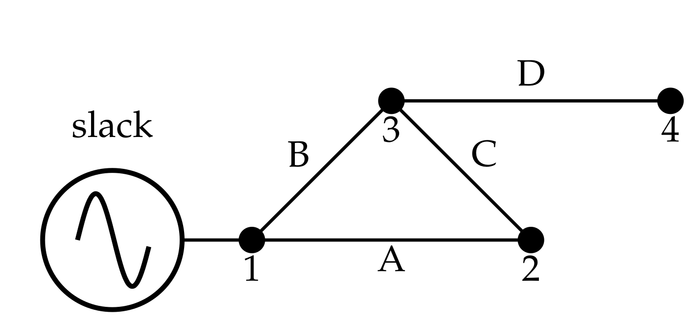In addition, the classical backward sweep by applying the Kirchhoff’s current law and the forward sweep by Kirchhoff’s voltage law are compared in a general power flow formula that makes both calculations in only one step [5]. To illustrate the general formulation of the matricial backward/forward power flow method, a small distribution system is chosen with some nodes, lines, and current flow directions that are defined. Next, the formulation process is detailed using the case study represented in Figure 2.  

Algorithm 1: General implementation of the HOA in the master stage.

From the electrical connection among nodes in Figure 2, it is possible to obtain the node-to-branch incidence matrix ($\mathbf{A}$) presented in Equation (13). Note that the rows of the matrix node-to-branch are assigned to the nodes in the following order, i.e., $1a,1b,1c,...,4a,4b,4c$, and in the columns, the lines ordered as $Aa,Ab,Ac,...,Da,Db,Dc$ are assigned, respectively. Note that each position of the matrix $\mathbf{A}$ is filled as follows:

✓

$A_{i\lambda ,j\gamma }=1$ if the node i in the phase $\lambda$ is the sending node for the line j in the phase $\gamma$;

✓

$A_{i\lambda ,j\gamma }=-1$ if the node i in the phase $\lambda$ is the receiving node for the line j in the phase $\gamma$;

✓

$A_{i\lambda ,j\gamma }=0$ if the node i is not connected with the line j.

Equation (13) shows the node-to-branch incidence matrix for the four-node test feeder in Figure 2:

$${\mathbf{A}}_{i\lambda ,j\gamma }=\left[\begin{array}{cccccccccccc}1& 0& 0& 1& 0& 0& 0& 0& 0& 0& 0& 0\\ 0& 1& 0& 0& 1& 0& 0& 0& 0& 0& 0& 0\\ 0& 0& 1& 0& 0& 1& 0& 0& 0& 0& 0& 0\\ -1& 0& 0& 0& 0& 0& 1& 0& 0& 0& 0& 0\\ 0& -1& 0& 0& 0& 0& 0& 1& 0& 0& 0& 0\\ 0& 0& -1& 0& 0& 0& 0& 0& 1& 0& 0& 0\\ 0& 0& 0& -1& 0& 0& -1& 0& 0& 1& 0& 0\\ 0& 0& 0& 0& -1& 0& 0& -1& 0& 0& 1& 0\\ 0& 0& 0& 0& 0& -1& 0& 0& -1& 0& 0& 1\\ 0& 0& 0& 0& 0& 0& 0& 0& 0& -1& 0& 0\\ 0& 0& 0& 0& 0& 0& 0& 0& 0& 0& -1& 0\\ 0& 0& 0& 0& 0& 0& 0& 0& 0& 0& 0& -1\end{array}\right]$$

(13)

where i corresponds to the node number, $\lambda$ to the node phase, j corresponds to the line, and $\gamma$ corresponds to the line phase. Note that nodes 1, 2, 3, and 4 are placed vertically along with the lines A, B, C, and D, respectively.

In order to obtain system voltage drops, the difference between each node per phase connected is carried out. If node 1 is located as the slack node, it reaches the subdivision of the matrix $\mathbf{A}$ in section ${\mathbf{A}}_s$ corresponding to the generator node and another area containing the demand nodes of system ${\mathbf{A}}_d$, as shown in Equation (14) [5].

$$\mathbf{A}=\left[\begin{array}{c}{\mathbf{A}}_{s3\varphi }\\ {\mathbf{A}}_{d3\varphi }\end{array}\right]$$

(14)

Equation (15) presents information related to the demanded drop voltage from the distribution network, where $E_{j\lambda }$ is the voltage drop between the extremes of each line for phase $\lambda$.

$$\begin{array}{cc}{E}_{Aa}& =V_{1a}-V_{2a}\\ E_{Ab}& =V_{1b}-V_{2b}\\ E_{Ac}& =V_{1c}-V_{2c}\\ E_{Ba}& =V_{1a}-V_{3a}\\ E_{Bb}& =V_{1b}-V_{3b}\\ E_{Bc}& =V_{1c}-V_{3c}\\ E_{Ca}& =V_{2a}-V_{3a}\\ E_{Cb}& =V_{2b}-V_{3b}\\ E_{Cc}& =V_{2c}-V_{3c}\\ E_{Da}& =V_{3a}-V_{4a}\\ E_{Db}& =V_{3b}-V_{4b}\\ E_{Dc}& =V_{3c}-V_{4c}\end{array}$$

(15)

For any general case and using the information of Equation (15), Equation (16) is used in a matrix form [43].

$${\mathbf{E}}_{b3\varphi }={\mathbf{A}}_{s3\varphi }^{\top }{V}_{s3\varphi }+{\mathbf{A}}_{d3\varphi }^{\top }{V}_{d3\varphi }$$

(16)

For application purposes, an initial voltage profile is assumed in which $V_{s3\varphi }={[11\angle -{120}^{\circ }1\angle {120}^{\circ }]}^{\top }$ and ${\mathbf{V}}_{d3\varphi }$ corresponds to all the demand nodes; in turn, E determines the potential drops in all system nodes.

Following Kirchhoff’s current law and the direction of currents in the network, Equation (17) is obtained.

$$\begin{array}{cc}{I}_{2a}=& I_{Ca}-I_{Aa}\\ I_{2b}=& I_{Cb}-I_{Ab}\\ I_{2c}=& I_{Cc}-I_{Ac}\\ I_{3a}=& -I_{Ba}-I_{Ca}+I_{Da}\\ I_{3a}=& -I_{Bb}-I_{Cb}+I_{Db}\\ I_{3a}=& -I_{Bc}-I_{Cc}+I_{Dc}\\ I_{4a}=& -I_{Da}\\ I_{4b}=& -I_{Db}\\ I_{4c}=& -I_{Dc}\end{array}$$

(17)

Observe that using the information in Equation (17), Equation (18) is determined in matrix form. [5].

$${\mathbf{I}}_{d3\varphi }={\mathbf{A}}_{d3\varphi }{\mathbf{I}}_{b3\varphi }$$

(18)

With the impedance matrix of the system employing Ohm’s law in [44], it is possible to determine the voltage drop per phase as shown in the matrix (19).

$$\left[\begin{array}{c}{E}_{Aa}\\ E_{Ab}\\ E_{Ac}\\ E_{Ba}\\ E_{Bb}\\ E_{Bc}\\ E_{Ca}\\ E_{Cb}\\ E_{Cc}\\ E_{Da}\\ E_{Db}\\ E_{Dc}\end{array}\right]=\left[\begin{array}{cccccccccccc}{Z}_{1a}& Z_{1b}& Z_{1c}& 0& 0& 0& 0& 0& 0& 0& 0& 0\\ Z_{1a}& Z_{1b}& Z_{1c}& 0& 0& 0& 0& 0& 0& 0& 0& 0\\ Z_{1a}& Z_{1b}& Z_{1c}& 0& 0& 0& 0& 0& 0& 0& 0& 0\\ 0& 0& 0& Z_{2a}& Z_{2b}& Z_{2c}& 0& 0& 0& 0& 0& 0\\ 0& 0& 0& Z_{2a}& Z_{2b}& Z_{2c}& 0& 0& 0& 0& 0& 0\\ 0& 0& 0& Z_{2a}& Z_{2b}& Z_{2c}& 0& 0& 0& 0& 0& 0\\ 0& 0& 0& 0& 0& 0& Z_{3a}& Z_{3b}& Z_{3c}& 0& 0& 0\\ 0& 0& 0& 0& 0& 0& Z_{3a}& Z_{3b}& Z_{3c}& 0& 0& 0\\ 0& 0& 0& 0& 0& 0& Z_{3a}& Z_{3b}& Z_{3c}& 0& 0& 0\\ 0& 0& 0& 0& 0& 0& 0& 0& 0& Z_{4a}& Z_{4b}& Z_{4c}\\ 0& 0& 0& 0& 0& 0& 0& 0& 0& Z_{4a}& Z_{4b}& Z_{4c}\\ 0& 0& 0& 0& 0& 0& 0& 0& 0& Z_{4a}& Z_{4b}& Z_{4c}\end{array}\right]\left[\begin{array}{c}{I}_{Aa}\\ I_{Ab}\\ I_{Ac}\\ I_{Ba}\\ I_{Bb}\\ I_{Bc}\\ I_{Ca}\\ I_{Cb}\\ I_{Cc}\\ I_{Da}\\ I_{Db}\\ I_{Dc}\end{array}\right]$$

(19)

With this information, Equation (20) is established in matrix form [43].

$${\mathbf{E}}_{b3\varphi }={\mathbf{Z}}_{b3\varphi }{\mathbf{I}}_{b3\varphi }$$

(20)

In the search to relate network demand voltages and currents, the adjacency matrix, which cannot be inverted, and the inverse impedance matrix are considered. From the line voltage of Equation (20), one can obtain the line currents and subsequently replace this expression in the demand currents (21), which results in an expression of demand node currents dependent on the adjacent matrix, line voltages, and impedances [6].

$${\mathbf{I}}_{d3\varphi }={\mathbf{A}}_{d3\varphi }{\mathbf{Z}}_{b3\varphi }^{-1}{\mathbf{E}}_{b3\varphi }$$

(21)

By using Equation (21), the slack node and demand nodes are obtained, which results in Equations (22) and (23) [43].

$${\mathbf{I}}_{d3\varphi }={\mathbf{A}}_{d3\varphi }{\mathbf{Z}}_{br\varphi }^{-1}\left({\mathbf{A}}_{s3\varphi }^{\top }{V}_{s3\varphi }+{\mathbf{A}}_{d3\varphi }^{\top }{V}_{d3\varphi }\right)$$

(22)

$${\mathbf{I}}_{d3\varphi }={\mathbf{Y}}_{ds3\varphi }{V}_{s3\varphi }+{\mathbf{Y}}_{dd3\varphi }{V}_{d3\varphi }$$

(23)

where $Y_{ds3\varphi }$ is equal to ${\mathbf{A}}_{d3\varphi }{\mathbf{Z}}_{b3\varphi }^{-1}{{\mathbf{A}}_{s3\varphi }}^T$, and ${\mathbf{Y}}_{dd3\varphi }$ equals ${\mathbf{A}}_{d3\varphi }{\mathbf{Z}}_{b3\varphi }^{-1}{\mathbf{A}}_{d3\varphi }^T$. Equation (24) reorganizes and determines the nodes’ stress [5].

$${\mathbf{V}}_{d3\varphi }=-{\mathbf{Y}}_{dd3\varphi }^{-1}\left({\mathbf{I}}_{d3\varphi }+{\mathbf{Y}}_{ds3\varphi }{\mathbf{V}}_{s3\varphi }\right)$$

(24)

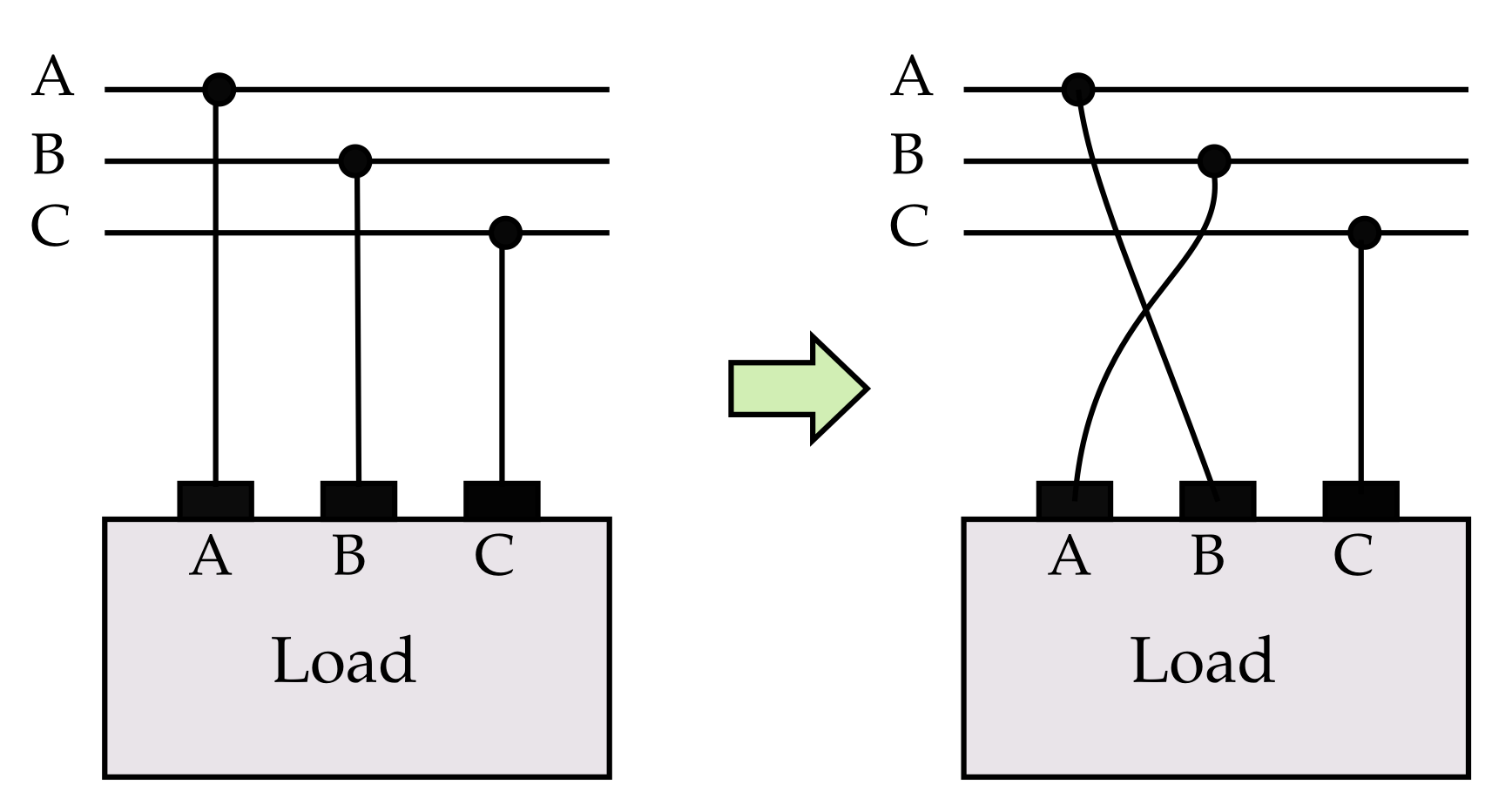
The three-phase demand current depends on whether the type of connection of the load is in $\Delta$ or Y (i.e., star connection); see Figure 3 for this case study, which is taken as reference for a kind of load in Y. Therefore, Equations (25)–(27) were selected. Likewise, Equations (28)–(30) are detailed if the type of load is in triangle [6].

$$I_{iA}={\left(\frac{S_{iA}}{V_{iA}}\right)}^{*}$$

(25)

$$I_{iB}={\left(\frac{S_{iB}}{V_{iB}}\right)}^{*}$$

(26)

$$I_{iC}={\left(\frac{S_{iC}}{V_{iC}}\right)}^{*}$$

(27)

$$I_{iA}={\left(\frac{S_{iAB}}{V_{iA}-V_{iB}}\right)}^{*}-{\left(\frac{S_{iCA}}{V_{iC}-V_{iA}}\right)}^{*}$$

(28)

$$I_{iB}={\left(\frac{S_{iBC}}{V_{iB}-V_{iC}}\right)}^{*}-{\left(\frac{S_{iAB}}{V_{iA}-V_{iB}}\right)}^{*}$$

(29)

$$I_{iC}={\left(\frac{S_{iCA}}{V_{iC}-V_{iA}}\right)}^{*}-{\left(\frac{S_{iBC}}{V_{iB}-V_{iC}}\right)}^{*}$$

(30)

Finally, using an iterative counter to solve Equation (24), Equation (31) is defined, where m is the iteration counter with values greater than 0.

$${\mathbf{V}}_{d3\varphi }^{m+1}=-{\mathbf{Y}}_{dd3\varphi }^{-1}\left({\mathbf{I}}_{d3\varphi }^m+{\mathbf{Y}}_{ds3\varphi }{\mathbf{V}}_{s3\varphi }\right)$$

(31)

Observe that the recursive formula in (31) converges to the power flow solution if the maximum difference between two consecutive voltage iterations is lower than the assigned tolerance [6].

Once the power flow Equations (2) and (3) are solved and the voltage in the demand nodes is determined, the three-phase power generation in the slack source can be easily calculated with Equation (32):

$${\mathbf{S}}_{s3\varphi }=\mathrm{diag}\left({\mathbf{V}}_{s3\varphi }\right)\left({\mathbf{Y}}_{ss3\varphi }^{*}{\mathbf{V}}_{s3\varphi }^{*}+{\mathbf{Y}}_{sd3\varphi }^{*}{\mathbf{V}}_{d3\varphi }^{*}\right)$$

(32)

where ${\mathbf{S}}_{s3\varphi }$ represents the complex three-phase power generation in the slack bus.

4. Power Systems under Study

In order to contrast the efficiency, robustness, and speed of the computational proposed HOA in Section 3 to solve the problem of the optimal phase-swapping in AC unbalanced distribution grids, the characteristics of the 8-, 25-, and 37-node radial three-phase distribution systems are presented below, which are proposed by [5].

4.1. Eight-Node Test System

This eight-node system is a distribution system with one slack node, seven lines, and seven demands, with a nominal voltage of 11 kV [45]. Figure 4 depicts this information.

Table A1. Load and line parameters for the eight-node system.

Line	Node i	Node j	Conductor	Length	${\mathit{P}}_{\mathit{jA}}$	${\mathit{Q}}_{\mathit{jA}}$	${\mathit{P}}_{\mathit{jB}}$	${\mathit{Q}}_{\mathit{jB}}$	${\mathit{P}}_{\mathit{jC}}$	${\mathit{Q}}_{\mathit{jC}}$
				[ft]	(kW)	(kvar)	(kW)	(kvar)	(kW)	(kvar)
1	1	2	1	5280	519	250	259	126	515	250
2	2	3	2	5280	0	0	259	126	486	235
3	2	5	3	5280	0	0	0	0	226	109
4	2	7	3	5280	486	235	0	0	0	0
5	3	4	4	5280	0	0	0	0	324	157
6	3	8	5	5280	0	0	267	129	0	0
7	5	6	6	5280	0	0	0	0	145	70

shows the values regarding the impedances by conductor type, along with the power consumption per phase in

Table A2. Impedance matrix for the type of conductors in the eight-node test system.

Conductor		Impedance Matrix ($\mathbf{\Omega }/$mi)
	$0.093654+j0.0402930$	$0.031218+j0.0134310$	$0.031218+j0.0134310$
1	$0.031218+j0.0134310$	$0.093654+j0.0402930$	$0.031218+j0.0134310$
	$0.031218+j0.0134310$	$0.031218+j0.0134310$	$0.093654+j0.0402930$
	$0.156090+j0.0671550$	$0.052030+j0.0223850$	$0.052030+j0.0223850$
2	$0.052030+j0.0223850$	$0.156090+j0.0671550$	$0.052030+j0.0223850$
	$0.052030+j0.0223850$	$0.052030+j0.0223850$	$0.156090+j0.0671550$
	$0.046827+j0.0201465$	$0.015609+j0.0067155$	$0.015609+j0.0067155$
3	$0.015609+j0.0067155$	$0.046827+j0.0201465$	$0.015609+j0.0067155$
	$0.015609+j0.0067155$	$0.015609+j0.0067155$	$0.046827+j0.0201465$
	$0.031218+j0.0134310$	$0.010406+j0.0044770$	$0.010406+j0.0044770$
4	$0.010406+j0.0044770$	$0.031218+j0.0134310$	$0.010406+j0.0044770$
	$0.010406+j0.0044770$	$0.010406+j0.0044770$	$0.031218+j0.0134310$
	$0.062436+j0.0268620$	$0.020812+j0.0089540$	$0.020812+j0.0089540$
5	$0.020812+j0.0089540$	$0.062436+j0.0268620$	$0.020812+j0.0089540$
	$0.020812+j0.0089540$	$0.020812+j0.0089540$	$0.062436+j0.0268620$
	$0.078045+j0.0335775$	$0.026015+j0.0111925$	$0.026015+j0.0111925$
6	$0.026015+j0.0111925$	$0.078045+j0.0335775$	$0.026015+j0.0111925$
	$0.026015+j0.0111925$	$0.026015+j0.0111925$	$0.078045+j0.0335775$

necessary in the phase-balance problem application.

4.2. 25-Node Test System

This test feeder is composed of 25 nodes, 24 distribution lines, and 22 consumer loads with a nominal voltage of 4.16 kV [46]. The electrical configuration of this test feeder is depicted in Figure 5. Note that the impedance parameters are listed in

Table A3. Load and line parameters for the 25-node system.

Line	Node i	Node j	Conductor	Length	${\mathit{P}}_{\mathit{jA}}$	${\mathit{Q}}_{\mathit{jA}}$	${\mathit{P}}_{\mathit{jB}}$	${\mathit{Q}}_{\mathit{jB}}$	${\mathit{P}}_{\mathit{jC}}$	${\mathit{Q}}_{\mathit{jC}}$
				[ft]	(kW)	(kvar)	(kW)	(kvar)	(kW)	(kvar)
1	1	2	1	1000	0	0	0	0	0	0
2	2	3	1	500	36	21.6	28.8	19.2	42	26.4
3	2	6	2	500	43.2	28.8	33.6	24	30	30
4	3	4	1	500	57.6	43.2	4.8	3.4	48	30
5	3	18	2	500	57.6	43.2	38.4	28.8	48	36
6	4	5	2	500	43.2	28.8	28.8	19.2	36	24
7	4	23	2	400	8.6	64.8	4.8	3.8	60	42
8	6	7	2	500	0	0	0	0	0	0
9	6	8	2	1000	43.2	28.8	28.8	19.2	3.6	2.4
10	7	9	2	500	72	50.4	38.4	28.8	48	30
11	7	14	2	500	57.6	36	38.4	28.8	60	42
12	7	16	2	500	57.6	4.3	3.8	28.8	48	36
13	9	10	2	500	36	21.6	28.8	19.2	32	26.4
14	10	11	2	300	50.4	31.7	24	14.4	36	24
15	11	12	3	200	57.6	36	48	33.6	48	36
16	11	13	3	200	64.8	21.6	33.6	21.1	36	24
17	14	15	2	300	7.2	4.3	4.8	2.9	6	3.6
18	14	17	3	300	57.6	43.2	33.6	24	54	38.4
19	18	20	2	500	50.4	36	38.4	28.8	54	38.4
20	18	21	3	400	5.8	4.3	3.4	2.4	5.4	3.8
21	20	19	3	400	8.6	6.5	4.8	3.4	6	4.8
22	21	22	3	400	72	50.4	57.6	43.2	60	48
23	23	24	2	400	50.4	36	43.2	30.7	4.8	3.6
24	24	25	3	400	8.6	6.5	4.8	2.9	6	4.2

together with power consumption per phase in

Table A4. Impedance matrix for the type of conductor in the 25-node test system.

Conductor		Impedance matrix ($\mathbf{\Omega }/$mi)
	$0.3686+j0.6852$	$0.0169+j0.1515$	$0.0155+j0.1098$
1	$0.0169+j0.1515$	$0.3757+j0.6715$	$0.0188+j0.2072$
	$0.0155+j0.1098$	$0.0188+j0.2072$	$0.3723+j0.6782$
	$0.9775+j0.8717$	$0.0167+j0.1697$	$0.0152+j0.1264$
2	$0.0167+j0.1697$	$0.9844+j0.8654$	$0.0186+j0.2275$
	$0.0152+j0.1264$	$0.0186+j0.2275$	$0.9810+j0.8648$
	$1.9280+j1.4194$	$0.0161+j0.1183$	$0.0161+j0.1183$
3	$0.0161+j0.1183$	$1.9308+j1.4215$	$0.0161+j0.1183$
	$0.0161+j0.1183$	$0.0161+j0.1183$	$1.9337+j1.4236$

.

4.3. IEEE 37-Node Test System

The unbalanced distribution system of 37 nodes, 36 demand nodes, 1 slack node, 35 lines, and 25 consumer loads with a nominal voltage of 4.80 kV [47] is represented in Figure 6. This system is located in California and is totally composed of subway lines, operating with an unbalanced transformer and a voltage regulator; for research, the transformers located at nodes 10 and 24 are disregarded. The voltage regulator located at nodes 1 and 2 is also replaced by an 1850 feet Type 1 conductor as proposed in [48]. Furthermore, it does not consider the transformer and the voltage regulator suggested by [8]. As in previous cases, the impedance parameters for the 37-bus system can be found in

Table A5. Load and line parameters for the IEEE 37-node system.

Line	Node i	Node j	Conductor	Length	${\mathit{P}}_{\mathit{jA}}$	${\mathit{Q}}_{\mathit{jA}}$	${\mathit{P}}_{\mathit{jB}}$	${\mathit{Q}}_{\mathit{jB}}$	${\mathit{P}}_{\mathit{jC}}$	${\mathit{Q}}_{\mathit{jC}}$
				[ft]	(kW)	(kvar)	(kW)	(kvar)	(kW)	(kvar)
1	1	2	1	1850	140	70	140	70	350	175
2	2	3	2	960	0	0	0	0	0	0
3	3	24	4	400	0	0	0	0	0	0
4	3	27	3	360	0	0	0	0	85	40
5	3	4	2	1320	0	0	0	0	0	0
6	4	5	4	240	0	0	0	0	42	21
7	4	9	3	600	0	0	0	0	85	40
8	5	6	3	280	42	21	0	0	0	0
9	6	7	4	200	42	21	42	21	42	21
10	6	8	4	280	42	21	0	0	0	0
11	9	10	3	200	0	0	0	0	0	0
12	10	23	3	600	0	0	85	40	0	0
13	10	11	3	320	0	0	0	0	0	0
14	11	13	3	320	85	40	0	0	0	0
15	11	12	4	320	0	0	0	0	42	21
16	13	14	3	560	0	0	0	0	42	21
17	14	18	3	640	140	70	0	0	0	0
18	14	15	4	520	0	0	0	0	0	0
19	15	16	4	200	0	0	0	0	85	40
20	15	17	4	1280	0	0	42	21	0	0
21	18	19	3	400	126	62	0	0	0	0
22	19	20	3	400	0	0	0	0	0	0
23	20	22	3	400	0	0	0	0	42	21
24	20	21	4	200	0	0	0	0	85	40
25	24	26	4	320	8	4	85	40	0	0
26	24	25	4	240	0	0	0	0	85	40
27	27	28	3	520	0	0	0	0	0	0
28	28	29	4	80	17	8	21	10	0	0
29	28	31	3	800	0	0	0	0	85	40
30	29	30	4	520	85	40	0	0	0	0
31	31	34	4	920	0	0	0	0	0	0
32	31	32	3	600	0	0	0	0	0	0
33	32	33	4	280	0	0	42	21	0	0
34	34	36	4	760	0	0	42	21	0	0
35	34	35	4	120	0	0	140	70	21	10

, along with the power consumption per phase in

Table A6. Data of impedance for the conductors used in the IEEE 37-bus system.

Conductor		Impedance Matrix ($\mathbf{\Omega }/$mi)
	$0.2926+j0.1973$	$0.0673-j0.0368$	$0.0337-j0.0417$
1	$0.0673-j0.0368$	$0.2646+j0.1900$	$0.0673-j0.0368$
	$0.0337-j0.0417$	$0.0673-j0.0368$	$0.2926+j0.1973$
	$0.4751+j0.2973$	$0.1629-j0.0326$	$0.1234-j0.0607$
2	$0.1629-j0.0326$	$0.4488+j0.2678$	$0.1629-j0.0326$
	$0.1234-j0.0607$	$0.1629-j0.0326$	$0.4751+j0.2973$
	$1.2936+j0.6713$	$0.4871+j0.2111$	$0.4585+j0.1521$
3	$0.4871+j0.2111$	$1.3022+j0.6326$	$0.4871+j0.2111$
	$0.4585+j0.1521$	$0.4871+j0.2111$	$1.2936+j0.6713$
	$2.0952+j0.7758$	$0.5204+j0.2738$	$0.4926+j0.2123$
4	$0.5204+j0.2738$	$2.1068+j0.7398$	$0.5204+j0.2738$
	$0.4926+j0.2123$	$0.5204+j0.2738$	$2.0952+j0.7758$

.

Note that, for the test systems, linear loads are directly included in the nodal admittance matrix, and all the demands are modeled as constant power terminals. In the same manner, the capacitive effect of the lines is denied based on their voltage level and length of the distribution lines [3].

5. Numerical Validation, Analysis, and Discussion

Next, the validation process of the master–slave optimization approach based on the HOA and the matricial backward/forward power flow method to solve the phase-swapping problem in unbalanced distribution networks is described.

5.1. Matricial Backward/Forward Power Flow Method Solution and Comparison

Different articles state the effectiveness of the iterative sweep method. Therefore, it was relevant to double-check the power losses in the 8-, 25-, and 37-node systems presented in

Table 2. Total and per phase active power losses for the IEEE 8-, IEEE 25-, and IEEE 37-node test feeders.

System under Test	Iterations	Processing Time (s)	Phase A	Phase B	Phase C	Total
			(kW)	(kW)	(kW)	(kW)
8	5	0.0905	1.7158	2.3305	9.9462	13.9925
25	9	0.1882	36.8801	14.7837	23.7570	75.4207
37	9	0.2919	27.1532	11.9143	37.0683	76.1357

.

From the results in Table 2, it is important to mention that the values of the power losses per phase and the total are the same as those reported in [5], where the power flow problem in three-phase asymmetric networks was solved with a new power flow approach named the triangular-based formulation.

By using master–slave optimization, it is possible to determine the best set of connections for the demand nodes using the phase-balancing method, achieving a reduction in the active phase and total losses based on the operating state of each system [5].

5.2. Parametrization of the Proposed HOA

The parametrization of the HOA to solve the studied problem is presented in

Table 3. General parameters for the computational implementation of HOA.

Hurricane optimization algorithm
Number of candidate solutions	12
Number of iterations	1000
Generation of solution candidates	Gaussian distribution
Matricial backward/forward power flow method
Number of iterations	1000
Error margin	$1\times {10}^{-10}$
Systems’ evaluation
Number of evaluations	100

.

As validated by [5], analysis sensitivity in the solution space is faster if the number of candidate solutions is reduced, but this also reduces the probability of finding the optimal global solution. Likewise, it occurs when candidate solutions are increased, where it is more likely to find a solution but one that affects processing time. The balance is between 500 and 1000 iterations with candidate solutions between 8 and 12, allowing the processing time to intersect with the possibility of finding the optimal global solution. For that reason, 1000 iterations and 12 candidate solutions are established for the proposed HOA algorithm. In addition, candidate solutions are generated through a randomized process, as recommended in [5]; 100 consecutive iterations are performed to determine the average time processing.

The results compared with the optimization methods were obtained using the MATLAB software (Version 2020a) together with the use of an Intel(R) Core (TM) i3-5005U CPU @2.00 GHz processor laptop with 8.00 GB of RAM running Windows 10 Home Single Language operating system of 64 bits.

It is worth mentioning that comparative methods are used, such as the DVSA proposed in [5] and the CBGA proposed in [3].

5.2.1. Eight-Node System Validation

In the study developed for the eight-node distribution system,

Table 4. Reference methods with their respective results in active power losses for the eight-node test feeder.

Method	Connections	Phase A	Phase B	Phase C	Total
		(kW)	(kW)	(kW)	(kW)
Benchmark case	{1, 1, 1, 1, 1, 1, 1}	1.7158	2.3305	9.9462	13.9925
CBGA	{6, 1, 5, 1, 4, 4, 1}	2.7295	4.0957	3.7617	10.5869
DVSA	{6, 1, 5, 1, 2, 1, 1}	2.7295	4.0957	3.7617	10.5869
HOA	{1, 6, 2, 1, 5, 3, 6}	3.8464	2.7412	3.9993	10.5869

displays the obtained results. This study carried out a comparison with the reference case, which includes DVSA and CBGA, respectively.

According to the results obtained in Table 4, there is a reduction of 24.34% as the optimum value for the HOA when compared to the benchmark case. Likewise, CBGA and DVSA algorithms obtained the same results [5]. The fact that all the methods reach the same reduction in the power losses is associated mainly with the size of the test system since the solution space for the IEEE 8-bus system is pretty small when compared with other test feeders.

An important result in Table 4 regards the diversity of the optimal solutions for the IEEE 8-bus system since the proposed HOA and the comparative methods find the same objective function value; however, each one of the codifications is different, producing different power losses per phase. This situation occurs since there exist some rotations in all loads that allow reaching the same global result.

To analyze the performance obtained with the HOA, Figure 7 displays the results obtained for phases A, B, and C, respectively.

Figure 7 shows that the performance of the voltage for each node phase is similar to that of the HOA method. Thus, the unbalance presented in the benchmark case is considerably reduced. Additionally, it is determined that Phase A presents a decrease in the slope between node-to-node stresses compared to the benchmark case. Likewise, the highest voltage drops are observed in nodes 3, 4, and 8, which are not the only ones to obtain a decrease. In Phase B, the opposite occurs because voltage drops increase but do not have a relevant change according to the reference voltage profile. In the graph corresponding to Phase C, the same pattern of Phase A occurs: a decrease in voltage drops in all the demanding nodes of the system.

Regarding processing times, it is worth emphasizing that, after 100 consecutive evaluations, the average processing time was 2.1184 s for the proposed HOA. This processing time is negligible for any practical application since the solution is reached very fast; however, it is mainly caused by the small size of the distribution grid since it has only eight nodes, which implies that each power flow evaluation takes milliseconds to be solved.

5.2.2. 25-Node System Validation

Table 5. Reference methods with their respective results in active power losses for the 25-node test feeder.

Method	Connections	Phase A	Phase B	Phase C	Total
		(kW)	(kW)	(kW)	(kW)
Benchmark case	{1,1,1,1,1,1,1,1,1,1,1,1,1,1,1,1,1,1,1,1,1,1,1,1}	36.8801	14.7837	23.757	75.4207
CBGA	{1,1,3,5,2,1,1,1,2,6,5,1,5,3,6,6,3,3,1,3,5,2,4,3}	25.7626	25.9510	20.5782	72.2919
DVSA	{1,2,4,5,6,1,2,3,1,5,4,3,3,5,5,2,3,3,5,4,2,2,2,3}	25.6645	26.1613	20.4630	72.2888
HOA	{3,6,3,2,6,4,4,6,1,5,4,3,3,5,5,2,3,6,1,3,5,5,3,4}	25.8208	26.0953	20.3704	72.2865

displays the results obtained for the 25-node distribution system for HOA, CBGA, DVSA, and their comparisons with the benchmark case.

Table 5 shows a reduction of 4.16% as the optimum value for HOA when compared with the benchmark case. It also presents a better result of 72.2865 kW concerning the related algorithms, which is an improvement with respect to the best result reported by DVSA in [5].

As occurring for the IEEE 8-bus system, all methodologies obtained considerably good results regarding the total power loss minimization; however, the difference between the DVSA and the HOA is about $2.30$W; even if this is a small reduction, it confirms the effectiveness of the HOA to solve the phase-swapping problem in three-phase networks. However, when the final solution of both algorithms are compared, it is possible to observe that the studied problem can have multiple near-optimal solutions with very different final load connections. This characteristic makes the phase-balancing problem one of the most complex optimization problems in electrical engineering, which makes it necessary to continue developing efficient optimization techniques to improve current literature results.

To analyze the performance obtained with the HOA, Figure 8 presents the voltage profile performances for the phases A, B, and C, respectively.

Figure 8 reveals that the performance of the voltage for each node phase is similar to the HOA method in a general manner so that the unbalance presented in the reference system has been reduced. Likewise, it is visible that Phase A presents a reduction in voltage drops, which is observed in all demand nodes. In Phase B, the opposite occurs because voltage drops increase in each node, causing an increase in voltage drops of the demand nodes. In the graph corresponding to Phase C, the same pattern of Phase A occurs: a decrease in voltage drops close to the reference voltage profile.

Regarding processing times, it is worth emphasizing that, after 100 consecutive evaluations, the average processing time was 55.0470 s for the proposed HOA, which can be considered to be negligible since it implies that, in one hour, it is possible to solve the studied problem about 6000 times in order to make a complete statistical analysis regarding the performance of the proposed optimization method; this is crucial in order to select the best solution (economically and technically) since, for this test feeder, there exist $4.7384\times {10}^{18}$ possible solutions.

5.2.3. IEEE 37-Node System Validation

For the IEEE 37-node distribution system,

Table 6. Reference methods with their respective results in active power losses for the IEEE 37-node test feeder.

Method	Connections	Phase A	Phase B	Phase C	Total
		(kW)	(kW)	(kW)	(kW)
Benchmark case	$\left[\begin{array}{c}1,1,1,1,1,1,1,1,1,1,1,1,1,1,1,1,1,1,\\ 1,1,1,1,1,1,1,1,1,1,1,1,1,1,1,1,1\end{array}\right]$	27.1532	11.9143	37.0683	76.1357
CBGA	$\left[\begin{array}{c}4,1,1,6,4,4,6,4,1,1,6,5,2,1,2,3,1,5,\\ 1,4,3,2,6,5,3,2,1,6,5,2,1,4,1,2,3\end{array}\right]$	19.9434	20.8957	20.739	61.5785
DVSA	$\left[\begin{array}{c}4,1,1,5,3,4,2,3,1,1,3,2,2,1,3,5,2,3,\\ 1,3,6,1,2,3,3,2,1,1,2,4,1,4,1,2,4\end{array}\right]$	21.0656	21.6989	18.7155	61.4801
HOA	$\left[\begin{array}{c}2,4,4,3,6,6,5,5,4,6,3,2,4,6,3,1,5,6,\\ 5,5,6,5,2,6,6,4,2,1,2,4,4,4,1,2,4\end{array}\right]$	21.1052	21.6956	18.6789	61.4797

presents the results obtained for HOA, CBGA, DVSA, and the reference case.

According to the results obtained in Table 6, HOA reaches a reduction of 19.25% regarding power losses when compared with the benchmark case. Likewise, CBGA and DVSA reach similar reductions with small variations lower than 0.13%. However, it must be emphasized that the HOA algorithm confirms its superiority when compared with DVSA and CBGA since it finds a better optimal solution for the IEEE 37-bus system, which happened with the previous test feeders.

To analyze the performance obtained with the HOA, Figure 9 establishes the results obtained in the phases A, B, and C regarding voltage profiles’ performance, respectively.

From Figure 9, it is evident that the voltage performance for each phase per node is similar to that in the HOA method. Thus, the unbalance presented in the reference system is minimized. Additionally, Phase A and Phase C increase the voltage at the nodes when having the base system as a reference. Nevertheless, the opposite occurs for Phase B because the voltage does not follow the other phases’ performance, causing an unbalance of the system, which is reflected in the reduction in the voltage profile relatve to the HOA’s balanced system. Regarding processing times, it is worth emphasizing that after 100 consecutive evaluations, the average processing time was 178.7548 s for the proposed HOA, which can be considered to be an excellent processing time taking into account that the solution space in this test feeder is about $1.0314\times {10}^{28}$; this implies that there exist millions of billions of possibilities to connect all loads in all nodes.

6. Conclusions

In this research, the problem of optimal phase-balancing in distribution networks considering a particular peak load scenario of operation was addressed through the application of a master–slave optimization methodology. In the master stage, the hurricane optimization algorithm was implemented to determine the set of nodal load connections using an integer codification with numbers 1 to 6 representing all the possibilities to connect loads per node, i.e., from connection ABC to connection BAC. In the slave stage, each one of the nodal connections provided by the HOA was evaluated through the matricial formulation of the backward/forward power flow method for three-phase asymmetric networks in order to determine the amount of power losses of each set of load connections. Numerical results in the 8-, 25-, and 37-bus systems demonstrated the effectiveness of the proposed optimization methodology with reductions of 24.43%, 4.15%, and 19.25%, with respect to the benchmark cases, respectively. Note that these results were important considering that these are equal or complement the literature reports with CBGA and DVSA, especially when taking into account that the solution spaces for each test feeder are $6^7$, $6^{2}4$, and $6^{3}6$, i.e., from a few hundred thousand to millions of billions of possible solutions.

Regarding processing times, the proposed HOA took about $2.1184$s, $55.0470$ s, and $178.7548$s to solve the optimal phase-swapping problem in the 8-, 25-, and IEEE 37-bus systems. These times are negligible, and these will permit the assessment of the studied problem (with low computational effort). This will ultimately help to find the best solution for the distribution companies considering technical and economical aspects prior to the physical implementation of the phase-balancing plan.

As future works, it will be possible to develop the following research studies:

✓

To consider, in the optimal phase-swapping problem, the effect of load curves (residential, industrial, commercial, and mixed behaviors) to determine the best optimal configuration that minimizes the total energy losses or its costs considering periods of time from days to months;

✓

To apply the proposed master–slave optimization method based on the HOA and the matricial backward/forward power flow method to the problem of the optimal selection of the calibers of conductors in three-phase asymmetric distribution networks;

✓

To extend the application of HOA to the problem of the optimal location and sizing of shunt devices in distribution networks, i.e., distribution static compensators, battery energy storage systems, and renewable generation, among others.

References

1. Cravioto, J.; Ohgaki, H.; Che, H.S.; Tan, C.; Kobayashi, S.; Toe, H.; Long, B.; Oudaya, E.; Rahim, N.A.; Farzeneh, H. The Effects of Rural Electrification on Quality of Life: A Southeast Asian Perspective. Energies 2020, 13, 2410. [Google Scholar] [CrossRef]
2. Dhivya, S.; Arul, R. Demand Side Management Studies on Distributed Energy Resources: A Survey. Trans. Energy Syst. Eng. Appl. 2021, 2, 17–31. [Google Scholar] [CrossRef]
3. Montoya, O.D.; Molina-Cabrera, A.; Grisales-Noreña, L.F.; Hincapié, R.A.; Granada, M. Improved Genetic Algorithm for Phase-Balancing in Three-Phase Distribution Networks: A Master-Slave Optimization Approach. Computation 2021, 9, 67. [Google Scholar] [CrossRef]
4. Soltani, S.; Rashidinejad, M.; Abdollahi, A. Dynamic phase balancing in the smart distribution networks. Int. J. Electr. Power Energy Syst. 2017, 93, 374–383. [Google Scholar] [CrossRef]
5. Cortés-Caicedo, B.; Avellaneda-Gómez, L.S.; Montoya, O.D.; Alvarado-Barrios, L.; Chamorro, H.R. Application of the Vortex Search Algorithm to the Phase-Balancing Problem in Distribution Systems. Energies 2021, 14, 1282. [Google Scholar] [CrossRef]
6. Cortés-Caicedo, B.; Avellaneda-Gómez, L.S.; Montoya, O.D.; Alvarado-Barrios, L.; Álvarez-Arroyo, C. An Improved Crow Search Algorithm Applied to the Phase Swapping Problem in Asymmetric Distribution Systems. Symmetry 2021, 13, 1329. [Google Scholar] [CrossRef]
7. Blasco, P.A.; Montoya-Mira, R.; Diez, J.M.; Montoya, R.; Reig, M.J. Compensation of Reactive Power and Unbalanced Power in Three-Phase Three-Wire Systems Connected to an Infinite Power Network. Appl. Sci. 2019, 10, 113. [Google Scholar] [CrossRef] [Green Version]
8. Granada-Echeverri, M.; Gallego-Rendón, R.A.; López-Lezama, J.M. Optimal Phase Balancing Planning for Loss Reduction in Distribution Systems using a Specialized Genetic Algorithm. Ing. Cienc. 2012, 8, 121–140. [Google Scholar] [CrossRef] [Green Version]
9. CREG. Resolucion 025 de 1995—Codigo de Redes; Technical Report; CREG: Bogotá D.C., Colombia, 1995. [Google Scholar]
10. Wu, J.; Liu, M.; Lu, W.; Xie, K. Real-time optimization of active distribution networks with distributed energy resources participating in frequency regulation. J. Clean. Prod. 2021, 328, 129597. [Google Scholar] [CrossRef]
11. Zhu, J.; Chow, M.Y.; Zhang, F. Phase balancing using mixed-integer programming [distribution feeders]. IEEE Trans. Power Syst. 1998, 13, 1487–1492. [Google Scholar] [CrossRef]
12. Zhu, J.; Bilbro, G.; Chow, M.Y. Phase balancing using simulated annealing. IEEE Trans. Power Syst. 1999, 14, 1508–1513. [Google Scholar] [CrossRef] [Green Version]
13. Chen, T.H.; Cherng, J.T. Optimal phase arrangement of distribution transformers connected to a primary feeder for system unbalance improvement and loss reduction using a genetic algorithm. In Proceedings of the 21st International Conference on Power Industry Computer Applications, Connecting Utilities, PICA 99, to the Millennium and Beyond (Cat. No.99CH36351), Santa Clara, CA, USA, 21–21 May 1999; IEEE: Piscataway, NJ, USA, 1999. [Google Scholar] [CrossRef]
14. Gandomkar, M. Phase balancing using genetic algorithm. In Proceedings of the 39th International Universities Power Engineering Conference, Bristol, UK, 6–8 September 2004; IEEE: Piscataway, NJ, USA, 2004; Volume 1, pp. 377–379. [Google Scholar]
15. Lin, C.; Chen, C.; Chuang, H.; Ho, C. Heuristic Rule-Based Phase Balancing of Distribution Systems by Considering Customer Load Patterns. IEEE Trans. Power Syst. 2005, 20, 709–716. [Google Scholar] [CrossRef]
16. Garcés-Ruiz, A.; Granada-Echeverri, M.; Rendon-Gallego, R.A. Phase-Balancing using ant colony optimization (In Spanish). Ingeniería Compet. 2011, 7, 43–52. [Google Scholar] [CrossRef]
17. Tuppadung, Y.; Kurutach, W. The Modified Particle Swarm Optimization for Phase Balancing. In Proceedings of the TENCON 2006—2006 IEEE Region 10 Conference, Hong Kong, China, 14–17 November 2006; IEEE: Piscataway, NJ, USA, 2006. [Google Scholar] [CrossRef]
18. Lin, C.H.; Chen, C.S.; Chuang, H.J.; Huang, M.Y.; Huang, C.W. An Expert System for Three-Phase Balancing of Distribution Feeders. IEEE Trans. Power Syst. 2008, 23, 1488–1496. [Google Scholar] [CrossRef]
19. Huang, M.Y.; Chen, C.S.; Lin, C.H.; Kang, M.S.; Chuang, H.J.; Huang, C.W. Three-phase balancing of distribution feeders using immune algorithm. IET Gener. Transm. Distrib. 2008, 2, 383. [Google Scholar] [CrossRef]
20. Kuo, C.C.; Chao, Y.T. Energy management based on AM/FM/GIS for phase balancing application on distribution systems. Energy Convers. Manag. 2010, 51, 485–492. [Google Scholar] [CrossRef]
21. Sathiskumar, M.; kumar, A.N.; Thiruvenkadam, S. Phase Balancing of Unbalanced Distribution Network through hybrid Greedy-Fuzzy Algorithm. Int. J. Comput. Appl. 2011, 34, 38–45. [Google Scholar] [CrossRef]
22. Sathiskumar, M.; kumar, A.N.; Lakshminarasimman, L.; Thiruvenkadam, S. A self adaptive hybrid differential evolution algorithm for phase balancing of unbalanced distribution system. Int. J. Electr. Power Energy Syst. 2012, 42, 91–97. [Google Scholar] [CrossRef]
23. Hooshmand, R.A.; Soltani, S. Fuzzy Optimal Phase Balancing of Radial and Meshed Distribution Networks Using BF-PSO Algorithm. IEEE Trans. Power Syst. 2012, 27, 47–57. [Google Scholar] [CrossRef]
24. Grigoras, G.; Gavrilas, M. Phase swapping of lateral branches from low-voltage distribution networks for load balancing. In Proceedings of the 2016 International Conference and Exposition on Electrical and Power Engineering (EPE), Iasi, Romania, 20–22 October 2016; IEEE: Piscataway, NJ, USA, 2016. [Google Scholar] [CrossRef]
25. Swapna, M.; Udaykumar, R.Y. An algorithm for optimal phase balancing of secondary distribution systems at each node. In Proceedings of the 2016 IEEE PES 13th International Conference on Transmission Distribution Construction, Operation Live-Line Maintenance (ESMO), Columbus, OH, USA, 12–15 September 2016; pp. 1–5. [Google Scholar] [CrossRef]
26. Toma, N.; Ivanov, O.; Neagu, B.; Gavrila, M. A PSO Algorithm for Phase Load Balancing in Low Voltage Distribution Networks. In Proceedings of the 2018 International Conference and Exposition on Electrical And Power Engineering (EPE), Iasi, Romania, 18–19 October 2018; pp. 0857–0862. [Google Scholar] [CrossRef]
27. Handhal, F.K.; Rashid, A.T. Load balancing in distribution system using heuristic search algorithm. In Proceedings of the 2018 International Conference on Advance of Sustainable Engineering and its Application (ICASEA), Wasit, Iraq, 14–15 March 2018; pp. 48–53. [Google Scholar] [CrossRef]
28. Rios, M.A.; Castaño, J.C.; Garcés, A.; Molina-Cabrera, A. Phase Balancing in Power Distribution Systems: A heuristic approach based on group-theory. In Proceedings of the 2019 IEEE Milan PowerTech, Milan, Italy, 23–27 June 2019; pp. 1–6. [Google Scholar] [CrossRef]
29. Gangwar, P.; Singh, S.N.; Chakrabarti, S. An Analytical Approach for Phase Balancing Considering Customer Load Profile. In Proceedings of the 2019 IEEE PES Innovative Smart Grid Technologies Europe (ISGT-Europe), Bucharest, Romania, 29 September–2 October 2019; pp. 1–5. [Google Scholar] [CrossRef]
30. Ivanov, O.; Neagu, B.C.; Gavrilas, M.; Grigoras, G.; Sfintes, C.V. Phase Load Balancing in Low Voltage Distribution Networks Using Metaheuristic Algorithms. In Proceedings of the 2019 International Conference on Electromechanical and Energy Systems (SIELMEN), Craiova, Romania, 9–11 October 2019; pp. 1–6. [Google Scholar] [CrossRef]
31. Garces, A.; Gil-González, W.; Montoya, O.D.; Chamorro, H.R.; Alvarado-Barrios, L. A Mixed-Integer Quadratic Formulation of the Phase-Balancing Problem in Residential Microgrids. Appl. Sci. 2021, 11, 1972. [Google Scholar] [CrossRef]
32. Kaur, S.; Kumbhar, G.; Sharma, J. A MINLP technique for optimal placement of multiple DG units in distribution systems. Int. J. Electr. Power Energy Syst. 2014, 63, 609–617. [Google Scholar] [CrossRef]
33. Anzola, D.; Castro, J.; Giral, D. Simulation tool for classical optimal flow analysis using Lagrange multipliers (In Spanish). Trans. Energy Syst. Eng. Appl. 2021, 2, 1–16. [Google Scholar] [CrossRef]
34. Montoya, O.D.; Alarcon-Villamil, J.A.; Hernández, J.C. Operating Cost Reduction in Distribution Networks Based on the Optimal Phase-Swapping including the Costs of the Working Groups and Energy Losses. Energies 2021, 14, 4535. [Google Scholar] [CrossRef]
35. Montoya, O.D.; Grisales-Noreña, L.F.; Rivas-Trujillo, E. Approximated Mixed-Integer Convex Model for Phase Balancing in Three-Phase Electric Networks. Computers 2021, 10, 109. [Google Scholar] [CrossRef]
36. Bruno, S.; Lamonaca, S.; Rotondo, G.; Stecchi, U.; Scala, M.L. Unbalanced Three-Phase Optimal Power Flow for Smart Grids. IEEE Trans. Ind. Electron. 2011, 58, 4504–4513. [Google Scholar] [CrossRef]
37. Montoya, O.D.; Arias-Londoño, A.; Grisales-Noreña, L.F.; Barrios, J.Á.; Chamorro, H.R. Optimal Demand Reconfiguration in Three-Phase Distribution Grids Using an MI-Convex Model. Symmetry 2021, 13, 1124. [Google Scholar] [CrossRef]
38. Rbouh, I.; El Imrani, A.A. Hurricane Search algorithm a new model for function optimization. In Proceedings of the 2014 5th International Conference on Information and Communication Systems (ICICS), Irbid, Jordan, 1–3 April 2014; pp. 1–5. [Google Scholar] [CrossRef]
39. Arteaga, J.A.; Montoya, O.D.; Grisales-Noreña, L.F. Solution of the optimal power flow problem in direct current grids applying the hurricane optimization algorithm. J. Phys. Conf. Ser. 2020, 1448, 012015. [Google Scholar] [CrossRef]
40. El-Sehiemy, R.A.; Rizk-Allah, R.M.; Attia, A.F. Assessment of hurricane versus sine-cosine optimization algorithms for economic/ecological emissions load dispatch problem. Int. Trans. Electr. Energy Syst. 2018, 29, e2716. [Google Scholar] [CrossRef]
41. Rizk-Allah, R.M.; El-Sehiemy, R.A.; Wang, G.G. A novel parallel hurricane optimization algorithm for secure emission/economic load dispatch solution. Appl. Soft Comput. 2018, 63, 206–222. [Google Scholar] [CrossRef]
42. Montoya, O.D.; Gil-González, W.; Giral, D.A. On the Matricial Formulation of Iterative Sweep Power Flow for Radial and Meshed Distribution Networks with Guarantee of Convergence. Appl. Sci. 2020, 10, 5802. [Google Scholar] [CrossRef]
43. Shen, T.; Li, Y.; Xiang, J. A Graph-Based Power Flow Method for Balanced Distribution Systems. Energies 2018, 11, 511. [Google Scholar] [CrossRef] [Green Version]
44. Elsaiah, S.; Benidris, M.; Mitra, J. A three-phase power flow solution method for unbalanced distribution networks. In Proceedings of the 2011 North American Power Symposium, Boston, MA, USA, 4–6 August 2011; pp. 1–8. [Google Scholar] [CrossRef]
45. Broadwater, R.P.; Chandrasekaran, A.; Huddleston, C.T.; Khan, A.H. Power flow analysis of unbalanced multiphase radial distribution systems. Electr. Power Syst. Res. 1988, 14, 23–33. [Google Scholar] [CrossRef]
46. Ramana, T.; Ganesh, V.; Sivanagaraju, S. Distributed Generator Placement And Sizing in Unbalanced Radial Distribution System. Cogener. Distrib. Gener. J. 2010, 25, 52–71. [Google Scholar] [CrossRef]
47. Singh, D.; Misra, R.K.; Mishra, S. Distribution system feeder re-phasing considering voltage-dependency of loads. Int. J. Electr. Power Energy Syst. 2016, 76, 107–119. [Google Scholar] [CrossRef]
48. Kersting, W. Radial distribution test feeders. IEEE Trans. Power Syst. 1991, 6, 975–985. [Google Scholar] [CrossRef]
Figure 1. An example of the load interchange in a particular node of the distribution network.
Computers 11 00043 g001
Figure 2. Example of a 4-node distribution grid with meshed structure.
Computers 11 00043 g002
Figure 3. Example of Δ and Y load connections.
Computers 11 00043 g003
Figure 4. Single-phase diagram of the 8-bus system.
Computers 11 00043 g004
Figure 5. Single-phase diagram of the 25-bus system.
Computers 11 00043 g005
Figure 6. Single-phase diagram of the 37-bus system.
Computers 11 00043 g006
Figure 7. Voltage profiles of the eight-node system of the phases A, B, and C in contrast to the benchmark case.
Computers 11 00043 g007
Figure 8. Voltage profiles of the 25-node system of phases A, B, and C in contrast to the benchmark case.
Computers 11 00043 g008
Figure 9. IEEE 37-node system voltage profiles of phases A, B, and C compared to the benchmark case.
Computers 11 00043 g009