
Comparison of On-Policy Deep Reinforcement Learning A2C with Off-Policy DQN in Irrigation Optimization: A Case Study at a Site in Portugal

 ,
,  , , , ,
  and
and
Abstract
:1. Introduction
2. Materials and Methods
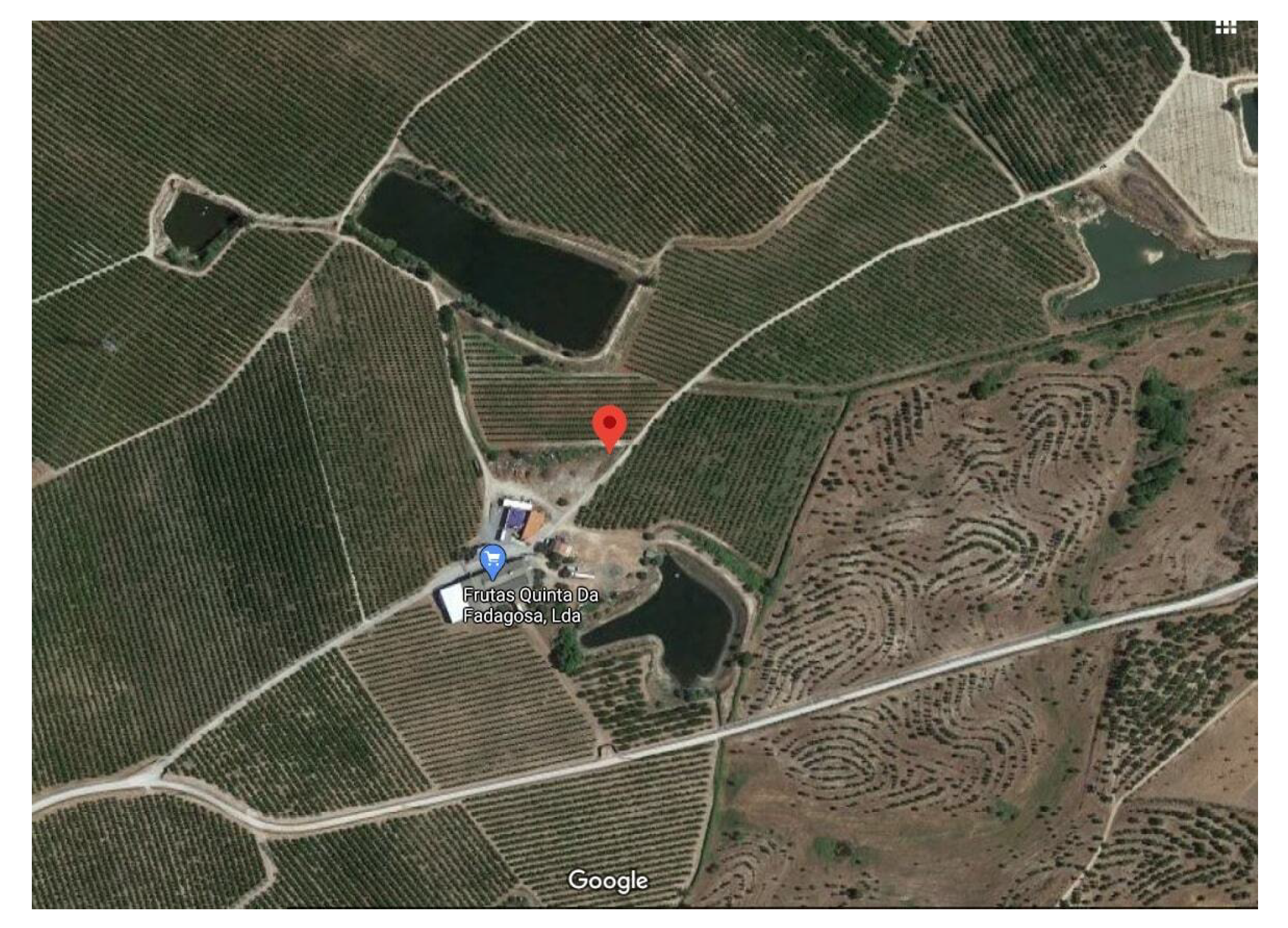
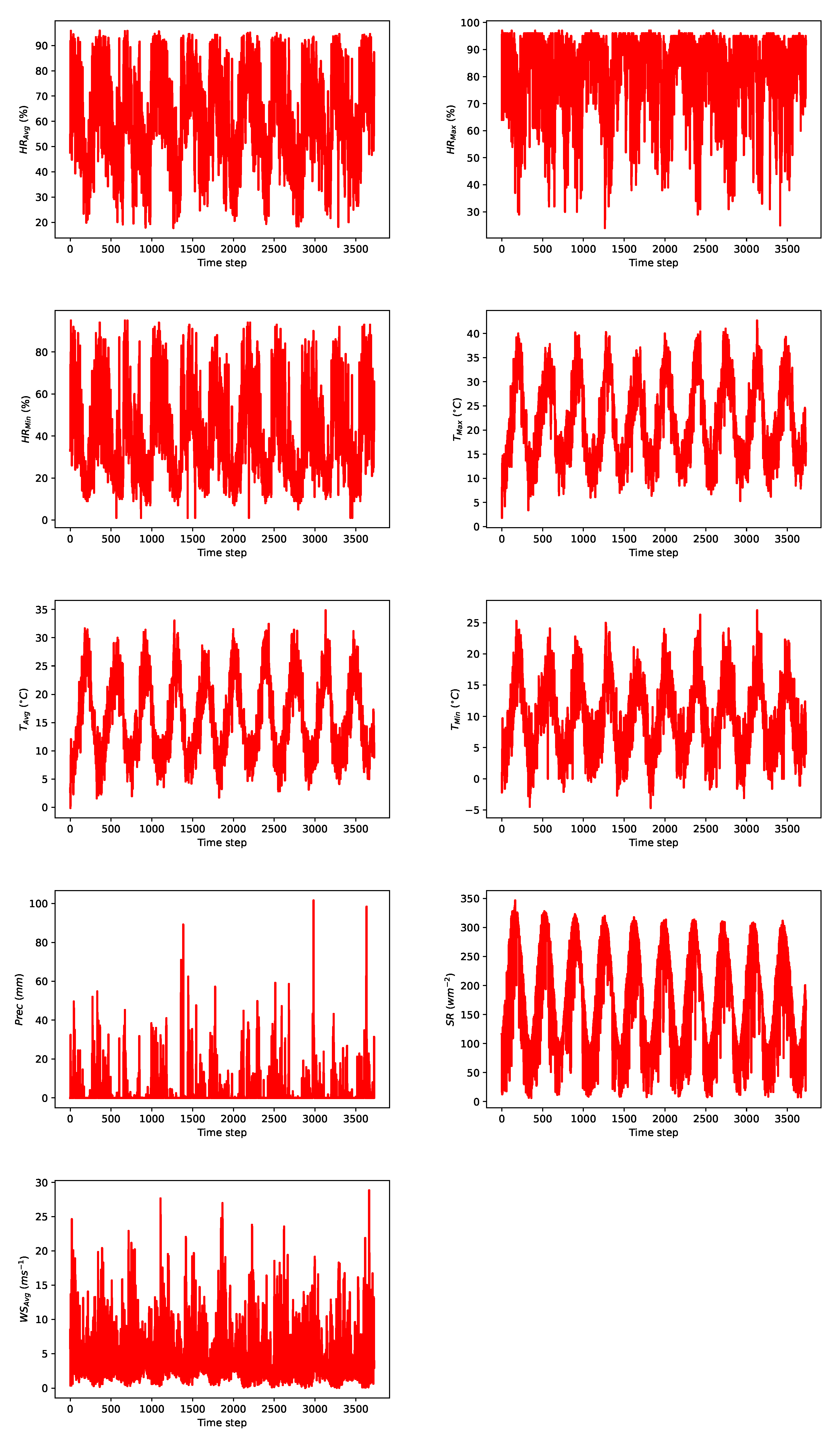
2.1. Data Collection
2.2. Data Pre-Processing
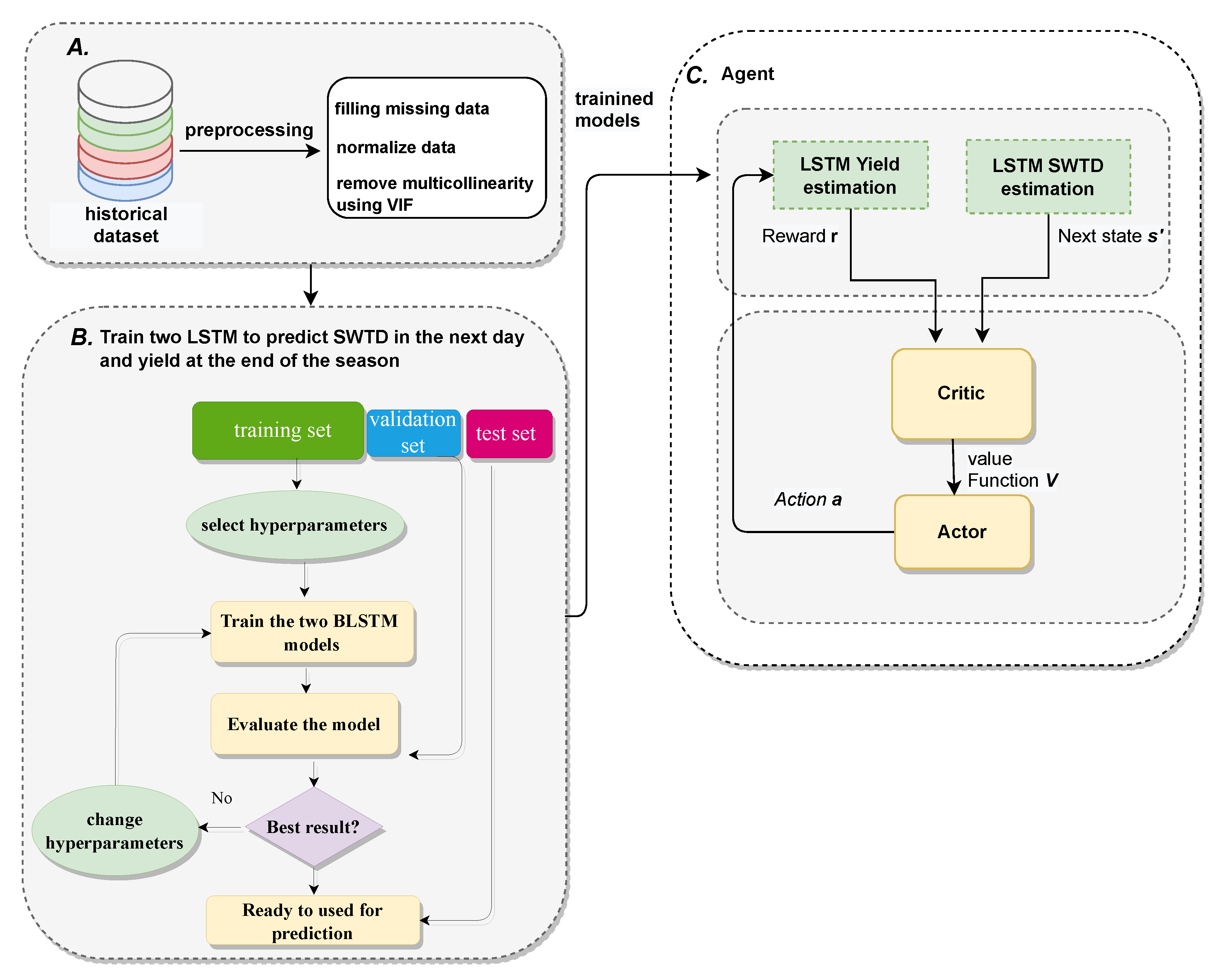
2.3. Model Used
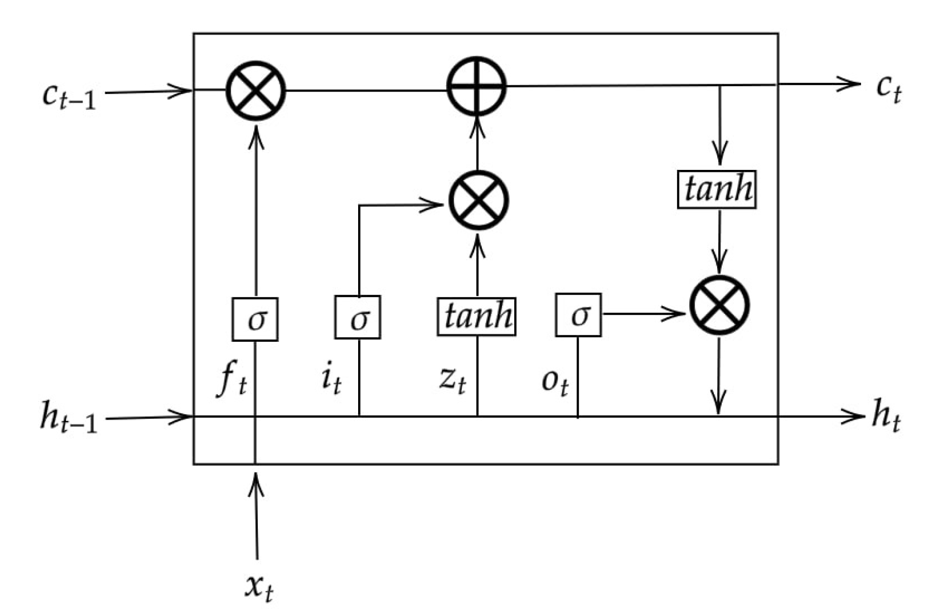
2.3.1. Bidirectional LSTM Structure
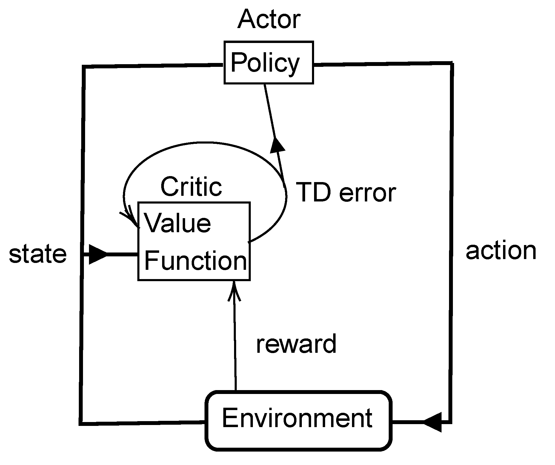
2.3.2. Advantage Actor–Critic Network
- States S: is the set of environment states.
- Action (A): a set of all possible actions.
- A real-valued function R of is called a reward function, which is an incentive mechanism that tells the agent which action is more valuable.
- A transition function P from to , where captures the probability of changing from state s to after executing action a.
2.4. Experimental Setup
2.4.1. States and Actions Setup
2.4.2. Environmental Setup

2.4.3. Training Configuration of Agent
| Algorithm 2: A2C Algorithm. |
 |
3. Results and Discussions
3.1. BLSTM Models Evaluation
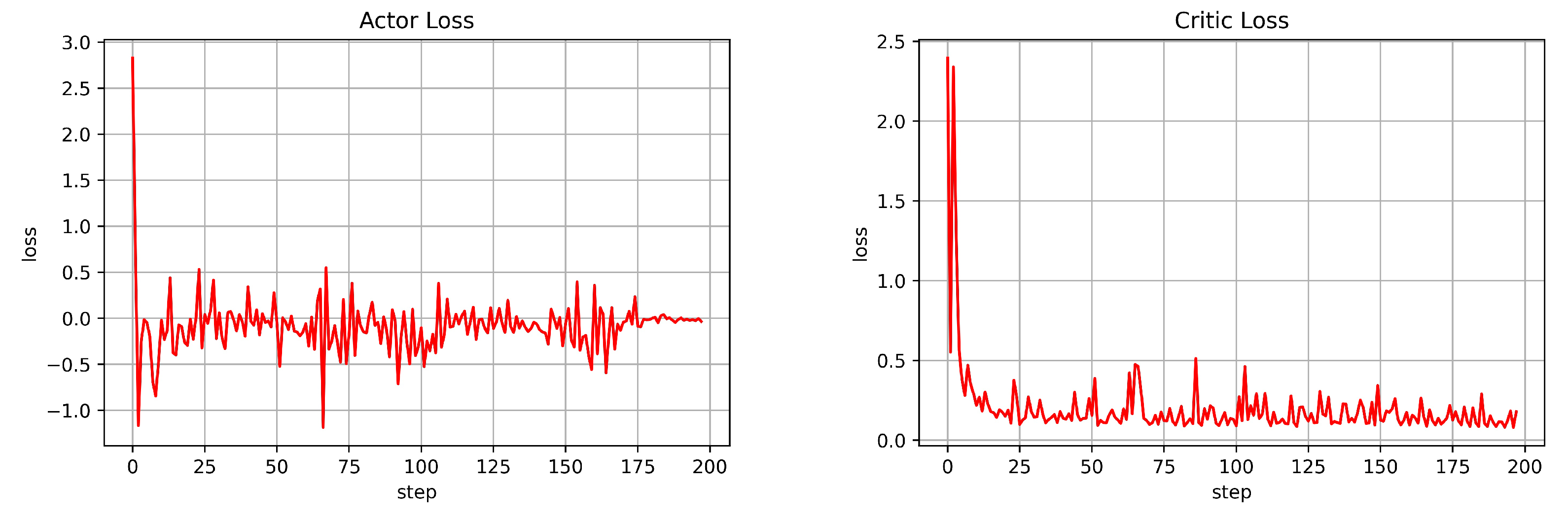
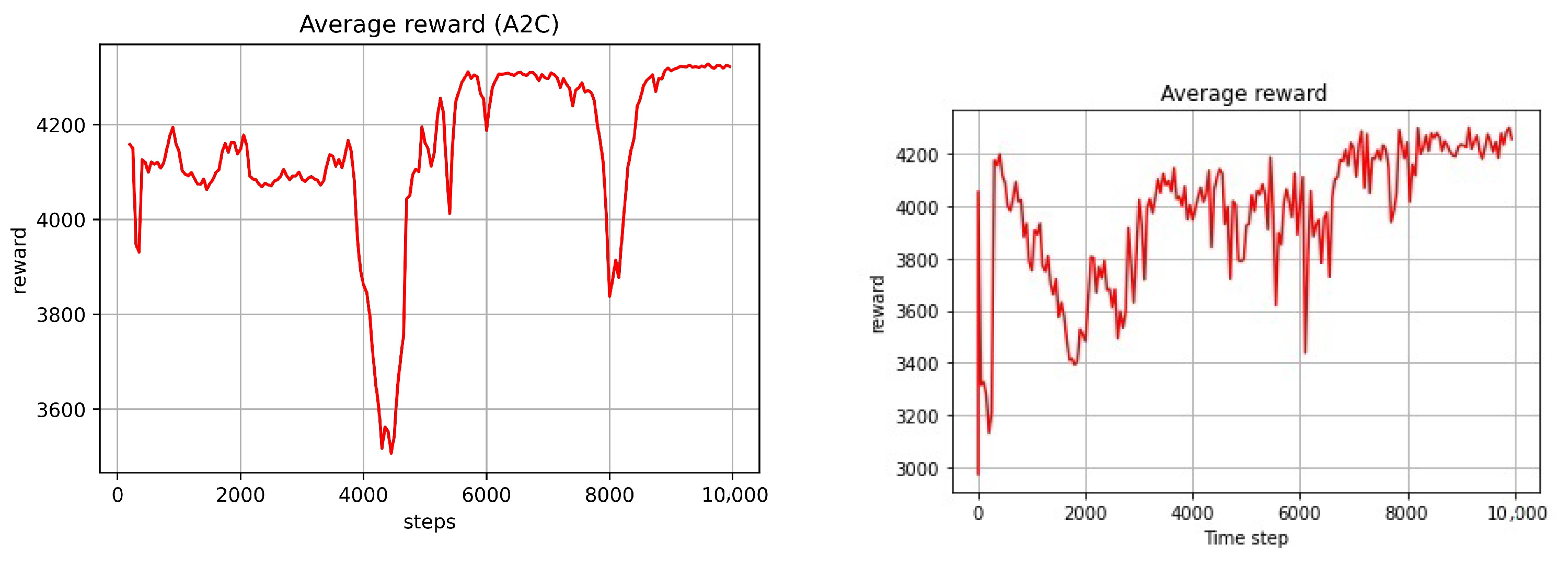
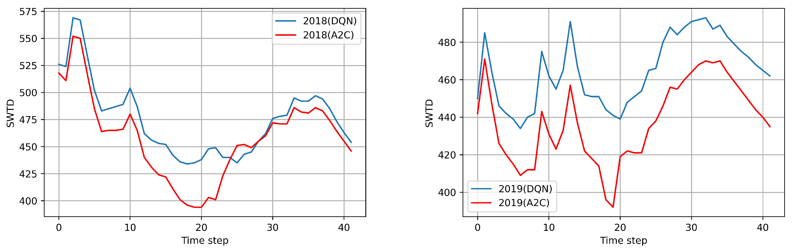
3.2. Evaluation of the A2C Agent
4. Conclusions
Author Contributions
Funding
Institutional Review Board Statement
Informed Consent Statement
Data Availability Statement
Acknowledgments
Conflicts of Interest
References
- Muimba-Kankolongo, A. Chapter 3–Factors Important to Crop Production. In Food Crop Production by Smallholder Farmers in Southern Africa; Muimba-Kankolongo, A., Ed.; Academic Press: Cambridge, MA, USA, 2018; pp. 15–21. [Google Scholar] [CrossRef]
- Fahad, S.; Bajwa, A.A.; Nazir, U.; Anjum, S.A.; Farooq, A.; Zohaib, A.; Sadia, S.; Nasim, W.; Adkins, S.; Saud, S.; et al. Crop Production under Drought and Heat Stress: Plant Responses and Management Options. Front. Plant Sci. 2017, 8. [Google Scholar] [CrossRef] [PubMed] [Green Version]
- FAO. World Agriculture 2030: Main Findings. 2002. Available online: http://www.fao.org/english/newsroom/news/2002/7833-en.html (accessed on 5 June 2020).
- Verdouw, C.; Wolfert, S.; Tekinerdogan, B. Internet of Things in agriculture. CAB Rev. 2016, 11, 1–12. [Google Scholar] [CrossRef]
- Lohchab, V.; Kumar, M.; Suryan, G.; Gautam, V.; Das, R.K. A Review of IoT based Smart Farm Monitoring. In Proceedings of the 2018 Second International Conference on Inventive Communication and Computational Technologies (ICICCT), Coimbatore, India, 20–21 April 2018; pp. 1620–1625. [Google Scholar] [CrossRef]
- Doshi, J.; Patel, T.; Bharti, S.K. Smart Farming using IoT, a solution for optimally monitoring farming conditions. Procedia Comput. Sci. 2019, 160, 746–751. [Google Scholar] [CrossRef]
- Shakya, A.K.; Ramola, A.; Kandwal, A.; Vidyarthi, A. Soil moisture sensor for agricultural applications inspired from state of art study of surfaces scattering models & semi-empirical soil moisture models. J. Saudi Soc. Agric. Sci. 2021, 20, 559–572. [Google Scholar] [CrossRef]
- Kumar Shakya, A.; Singh, S. Design of novel Penta core PCF SPR RI sensor based on fusion of IMD and EMD techniques for analysis of water and transformer oil. Measurement 2022, 188, 110513. [Google Scholar] [CrossRef]
- Abioye, E.A.; Hensel, O.; Esau, T.J.; Elijah, O.; Abidin, M.S.Z.; Ayobami, A.S.; Yerima, O.; Nasirahmadi, A. Precision Irrigation Management Using Machine Learning and Digital Farming Solutions. AgriEngineering 2022, 4, 70–103. [Google Scholar] [CrossRef]
- Liakos, K.; Busato, P.B.; Moshou, D.; Pearson, S.; Bochtis, D. Machine Learning in Agriculture: A Review. Sensors 2018, 18, 2674. [Google Scholar] [CrossRef] [Green Version]
- Kamilaris, A.; Prenafeta-Boldú, F.X. Deep learning in agriculture: A survey. Comput. Electron. Agric. 2018, 147, 70–90. [Google Scholar] [CrossRef] [Green Version]
- Alibabaei, K.; Gaspar, P.D.; Lima, T.M.; Campos, R.M.; Girão, I.; Monteiro, J.; Lopes, C.M. A Review of the Challenges of Using Deep Learning Algorithms to Support Decision-Making in Agricultural Activities. Remote Sens. 2022, 14, 638. [Google Scholar] [CrossRef]
- Nguyen, G.; Dlugolinsky, S.; Bobak, M.; Tran, V.; Garcia, A.L.; Heredia, I.; Malik, P.; Hluchy, L. Machine Learning and Deep Learning frameworks and libraries for large-scale data mining: A survey. Artif. Intell. Rev. 2019, 52, 77–124. [Google Scholar] [CrossRef] [Green Version]
- Min, E.; Guo, X.; Liu, Q.; Zhang, G.; Cui, J.; Long, J. A Survey of Clustering with Deep Learning: From the Perspective of Network Architecture. IEEE Access 2018, 6, 39501–39514. [Google Scholar] [CrossRef]
- Zia, H.; Rehman, A.; Harris, N.R.; Fatima, S.; Khurram, M. An Experimental Comparison of IoT-Based and Traditional Irrigation Scheduling on a Flood-Irrigated Subtropical Lemon Farm. Sensors 2021, 21, 4175. [Google Scholar] [CrossRef] [PubMed]
- Tseng, D.; Wang, D.; Chen, C.; Miller, L.; Song, W.; Viers, J.; Vougioukas, S.; Carpin, S.; Ojea, J.A.; Goldberg, K. Towards Automating Precision Irrigation: Deep Learning to Infer Local Soil Moisture Conditions from Synthetic Aerial Agricultural Images. In Proceedings of the 2018 IEEE 14th International Conference on Automation Science and Engineering (CASE), Munich, Germany, 20–24 August 2018; pp. 284–291. [Google Scholar]
- Song, X.; Zhang, G.; Liu, F.; Li, D.; Zhao, Y.; Yang, J. Modeling spatio-temporal distribution of soil moisture by deep learning-based cellular automata model. J. Arid. Land 2016, 8, 734–748. [Google Scholar] [CrossRef] [Green Version]
- Saggi, M.K.; Jain, S. Reference evapotranspiration estimation and modeling of the Punjab Northern India using deep learning. Comput. Electron. Agric. 2019, 156, 387–398. [Google Scholar] [CrossRef]
- de Oliveira e Lucas, P.; Alves, M.A.; de Lima e Silva, P.C.; Guimarães, F.G. Reference evapotranspiration time series forecasting with ensemble of convolutional neural networks. Comput. Electron. Agric. 2020, 177, 105700. [Google Scholar] [CrossRef]
- Ahmed, A.A.M.; Deo, R.C.; Raj, N.; Ghahramani, A.; Feng, Q.; Yin, Z.; Yang, L. Deep Learning Forecasts of Soil Moisture: Convolutional Neural Network and Gated Recurrent Unit Models Coupled with Satellite-Derived MODIS, Observations and Synoptic-Scale Climate Index Data. Remote Sens. 2021, 13, 554. [Google Scholar] [CrossRef]
- Adab, H.; Morbidelli, R.; Saltalippi, C.; Moradian, M.; Ghalhari, G.A.F. Machine Learning to Estimate Surface Soil Moisture from Remote Sensing Data. Water 2020, 12, 3223. [Google Scholar] [CrossRef]
- Jimenez, A.F.; Ortiz, V.B.; Bondesan, L.; Morata, G.; Damianidis, D. Evaluation of two recurrent neural network methods for prediction of irrigation rate and timing. Trans. ASABE 2020, 63, 1327–1348. [Google Scholar] [CrossRef]
- Bu, F.; Wang, X. A smart agriculture IoT system based on deep reinforcement learning. Future Gener. Comput. Syst. 2019, 99, 500–507. [Google Scholar] [CrossRef]
- Chen, M.; Cui, Y.; Wang, X.; Xie, H.; Liu, F.; Luo, T.; Zheng, S.; Luo, Y. A reinforcement learning approach to irrigation decision-making for rice using weather forecasts. Agric. Water Manag. 2021, 250, 106838. [Google Scholar] [CrossRef]
- Alibabaei, K.; Gaspar, P.D.; Assunção, E.; Alirezazadeh, S.; Lima, T.M. Irrigation optimization with a deep reinforcement learning model: Case study on a site in Portugal. Agric. Water Manag. 2022, 263, 107480. [Google Scholar] [CrossRef]
- Mnih, V.; Badia, A.P.; Mirza, M.; Graves, A.; Harley, T.; Lillicrap, T.P.; Silver, D.; Kavukcuoglu, K. Asynchronous Methods for Deep Reinforcement Learning. In Proceedings of the 33rd International Conference on Machine Learning, PMLR, New York, NY, USA, 19–24 June 2016, Volume 48. pp. 1928–1937.
- Hoogenboom, G.; Porter, C.H.; Boote, K.J.; Shelia, V.; Wilkens, P.W.; Singh, U.; White, J.W.; Asseng, S.; Lizaso, J.I.; Cadena, P.M.; et al. The DSSAT crop modeling ecosystem. In Advances in Crop Modelling for a Sustainable Agriculture; Burleigh Dodds Science Publishing: Cambridge, UK, 2019; pp. 173–216. [Google Scholar] [CrossRef]
- Hoogenboom, G.; Porter, C.; Shelia, V.; Boote, K.; Singh, U.; White, J.; Hunt, L.; Ogoshi, R.; Lizaso, J.; Koo, J.; et al. Decision Support System for Agrotechnology Transfer (DSSAT) Version 4.7.5; DSSAT Foundation: Gainesville, FL, USA, 2019. [Google Scholar]
- Alibabaei, K.; Gaspar, P.D.; Lima, T.M. Crop Yield Estimation Using Deep Learning Based on Climate Big Data and Irrigation Scheduling. Energies 2021, 14, 3004. [Google Scholar] [CrossRef]
- Allen, R.G.; Pereira, L.S.; Raes, M.S.D. Crop Evapotranspiration–Guidelines for Computing Crop Water Requirements FAO Irrigation and Drainage Paper 56; FAO–Food and Agriculture Organization of the United Nations: Rome, Italy, 1998. [Google Scholar]
- Montgomery, D.C.; Jennings, C.L.; Kulahci, M. Introduction to Time Series Analysis and Forecasting; Wiley Series in Probability and Statistics; Wiley: Hoboken, NJ, USA, 2011. [Google Scholar]
- James, G.; Witten, D.; Hastie, T.; Tibshirani, R. An Introduction to Statistical Learning: With Applications in R; Springer Publishing Company, Incorporated: Berlin/Heidelberg, Germany, 2014. [Google Scholar]
- Jain, L.C.; Medsker, L.R. Recurrent Neural Networks: Design and Applications, 1st ed.; CRC Press, Inc.: Boca Raton, FL, USA, 1999. [Google Scholar]
- Willmott, C.J.; Ackleson, S.G.; Davis, R.E.; Feddema, J.J.; Klink, K.M.; Legates, D.R.; O’Donnell, J.; Rowe, C.M. Statistics for the evaluation and comparison of models. J. Geophys. Res. Ocean. 1985, 90, 8995–9005. [Google Scholar] [CrossRef] [Green Version]
- Sutton, R.S.; Barto, A.G. Reinforcement Learning: An Introduction, 2nd ed.; The MIT Press: Cambridge, MA, USA, 2018. [Google Scholar]
- Konda, V.R.; Tsitsiklis, J.N. Actor–Critic Algorithms; MIT Press: Cambridge, MA, USA, 2000; pp. 1008–1014. [Google Scholar]
- Sutton, R.S. Learning to Predict by the Methods of Temporal Differences. Mach. Learn. 1988, 3, 9–44. [Google Scholar] [CrossRef]
- Grondman, I.; Busoniu, L.; Lopes, G.A.D.; Babuska, R. A Survey of Actor–Critic Reinforcement Learning: Standard and Natural Policy Gradients. IEEE Trans. Syst. Man Cybern. Part C Appl. Rev. 2012, 42, 1291–1307. [Google Scholar] [CrossRef] [Green Version]
- Williams, R.J.; Peng, J. Function Optimization using Connectionist Reinforcement Learning Algorithms. Connect. Sci. 1991, 3, 241–268. [Google Scholar] [CrossRef]
- Mnih, V.; Kavukcuoglu, K.; Silver, D.; Graves, A.; Antonoglou, I.; Wierstra, D.; Riedmiller, M. Playing Atari with Deep Reinforcement Learning. arXiv 2013, arXiv:1312.5602. [Google Scholar]
- Abadi, M.; Agarwal, A.; Barham, P.; Brevdo, E.; Chen, Z.; Citro, C.; Corrado, G.S.; Davis, A.; Dean, J.; Devin, M.; et al. TensorFlow: Large-Scale Machine Learning on Heterogeneous Systems. 2015. Available online: tensorflow.org (accessed on 1 December 2020).
- Chollet, F. 2015. Available online: https://keras.io (accessed on 1 December 2020).
- Alibabaei, K.; Gaspar, P.D.; Lima, T.M. Modeling Soil Water Content and Reference Evapotranspiration from Climate Data Using Deep Learning Method. Appl. Sci. 2021, 11, 5029. [Google Scholar] [CrossRef]
- Patterson, J.; Gibson, A. Deep Learning: A Practitioner’s Approach; O’Reilly Media: Sebastopol, CA, USA, 2017. [Google Scholar]
- Rodrigues, L.C. Water Resources Fee in Portugali, 2016. Led by the Institute for European Environmental Policy. Available online: https://ieep.eu/ (accessed on 1 July 2020).


| Variables | Unit | Data Source | Max | Min | Mean | SD |
|---|---|---|---|---|---|---|
| % | DRAP-Centro | 95 | 0 | 38.72 | 20.20 | |
| % | DRAP-Centro | 97 | 24 | 81.29 | 15.05 | |
| % | DRAP-Centro | 95.89 | 27.75 | 60.38 | 18.78 | |
| C | DRAP-Centro | 27 | −4.7 | 9.76 | 5.63 | |
| C | DRAP-Centro | 42.7 | 1.8 | 21.84 | 8.42 | |
| C | DRAP-Centro | 34.84 | −0.12 | 15.68 | 6.90 | |
| ms | DRAP-Centro | 86.5 | 3.5 | 24.67 | 10.61 | |
| ms | DRAP-Centro | 28.85 | 0.031 | 4.62 | 3.80 | |
| mm | DRAP-Centro | 101.6 | 0 | 2.28 | 7.20 | |
| wm | DRAP-Centro | 346.66 | 6.35 | 172.02 | 89.25 | |
| mm d | Penman-Monteith | 9.8 | 0.2 | 3.68 | 2.088 | |
| equation (AquaCrop calculator) | ||||||
| Tomato yield | kg/ha | DSSAT | 8387 | 974 | 4391 | 2564 |
| Environment states | , , , , , , |
| Set of actions | 0, 10, 15, 20, 25, 30, 35, 40, 45, 50, 55, 60 |
| Model | No. Layers | No. Hidden Layers | Batch Size | Learning Rate | Decay | Drop Out Size Out Size |
|---|---|---|---|---|---|---|
| BLSTM1 | 2 | 512 | 64 | 0.3 | ||
| BLSTM2 | 1 | 512 | 124 | 0.2 |
| Param | Explanation |
|---|---|
| action | Amount of water for irrigation |
| state | Climate data and SWTD |
| Done | A boolean value. If true, it indicates the end of the season |
| next_SWTD | SWTD after irrigation |
| time_step | The day of the season |
| Irrigation | Yield (kg/ha) | Total Irrigation (ha-mm/ha) | Net Return (dollars/ha) |
|---|---|---|---|
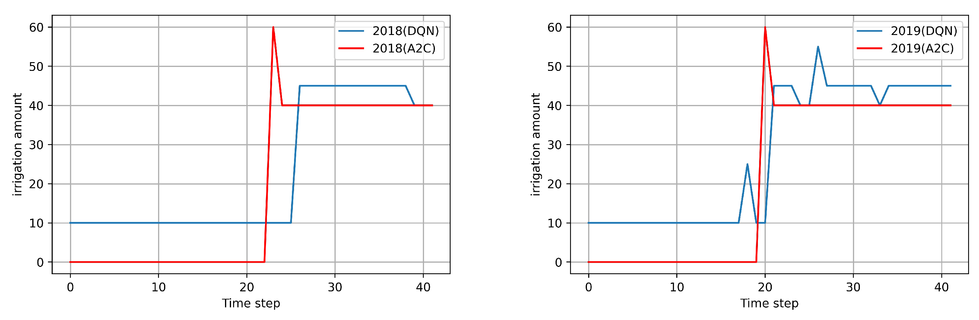
| A2C (2018) | 4475 | 780 | 3202 |
| DQN (2018) | 4675 (3% ↑) | 965 (20% ↑) | 3270 (3% ↑) |
| threshold of 480 with Fixed 50 mm (2018) | 5000 (7.5% ↑) | 1400 (45% ↑) | 3306 (3% ↑) |
| A2C (2019) | 3787 | 900 | 2559 |
| DQN (2019) | 4046.6 (7% ↑) | 1165(23% ↑) | 2666(4% ↑) |
| threshold of 480 with Fixed 50 mm (2019) | 4395 (14% ↑) | 1800 (50% ↑) | 2628 (2.6% ↑) |
Publisher’s Note: MDPI stays neutral with regard to jurisdictional claims in published maps and institutional affiliations. |
© 2022 by the authors. Licensee MDPI, Basel, Switzerland. This article is an open access article distributed under the terms and conditions of the Creative Commons Attribution (CC BY) license (https://creativecommons.org/licenses/by/4.0/).
Share and Cite
Alibabaei, K.; Gaspar, P.D.; Assunção, E.; Alirezazadeh, S.; Lima, T.M.; Soares, V.N.G.J.; Caldeira, J.M.L.P. Comparison of On-Policy Deep Reinforcement Learning A2C with Off-Policy DQN in Irrigation Optimization: A Case Study at a Site in Portugal. Computers 2022, 11, 104. https://0-doi-org.brum.beds.ac.uk/10.3390/computers11070104
Alibabaei K, Gaspar PD, Assunção E, Alirezazadeh S, Lima TM, Soares VNGJ, Caldeira JMLP. Comparison of On-Policy Deep Reinforcement Learning A2C with Off-Policy DQN in Irrigation Optimization: A Case Study at a Site in Portugal. Computers. 2022; 11(7):104. https://0-doi-org.brum.beds.ac.uk/10.3390/computers11070104
Chicago/Turabian StyleAlibabaei, Khadijeh, Pedro D. Gaspar, Eduardo Assunção, Saeid Alirezazadeh, Tânia M. Lima, Vasco N. G. J. Soares, and João M. L. P. Caldeira. 2022. "Comparison of On-Policy Deep Reinforcement Learning A2C with Off-Policy DQN in Irrigation Optimization: A Case Study at a Site in Portugal" Computers 11, no. 7: 104. https://0-doi-org.brum.beds.ac.uk/10.3390/computers11070104