Classification of Vowels from Imagined Speech with Convolutional Neural Networks

Institute of Computer Science, University of Tartu, Ülikooli 18, 50090 Tartu, Estonia
*
Author to whom correspondence should be addressed.
Computers 2020, 9(2), 46; https://0-doi-org.brum.beds.ac.uk/10.3390/computers9020046
Submission received: 12 May 2020
/
Revised: 26 May 2020
/
Accepted: 27 May 2020
/
Published: 1 June 2020
(This article belongs to the Special Issue Machine Learning for EEG Signal Processing)
Abstract
:Imagined speech is a relatively new electroencephalography (EEG) neuro-paradigm, which has seen little use in Brain-Computer Interface (BCI) applications. Imagined speech can be used to allow physically impaired patients to communicate and to use smart devices by imagining desired commands and then detecting and executing those commands in a smart device. The goal of this research is to verify previous classification attempts made and then design a new, more efficient neural network that is noticeably less complex (fewer number of layers) that still achieves a comparable classification accuracy. The classifiers are designed to distinguish between EEG signal patterns corresponding to imagined speech of different vowels and words. This research uses a dataset that consists of 15 subjects imagining saying the five main vowels (a, e, i, o, u) and six different words. Two previous studies on imagined speech classifications are verified as those studies used the same dataset used here. The replicated results are compared. The main goal of this study is to take the proposed convolutional neural network (CNN) model from one of the replicated studies and make it much more simpler and less complex, while attempting to retain a similar accuracy. The pre-processing of data is described and a new CNN classifier with three different transfer learning methods is described and used to classify EEG signals. Classification accuracy is used as the performance metric. The new proposed CNN, which uses half as many layers and less complex pre-processing methods, achieved a considerably lower accuracy, but still managed to outperform the initial model proposed by the authors of the dataset by a considerable margin. It is recommended that further studies investigating classifying imagined speech should use more data and more powerful machine learning techniques. Transfer learning proved beneficial and should be used to improve the effectiveness of neural networks.
1. Introduction
Electroencephalography (EEG) has seen a number of high-profile advances made in recent times, like robot tracking through mind control [1] and speech synthesis from neural signals [2]. One interesting area of EEG research is imagined speech. Imagined speech is the act of internally pronouncing words or letters without actually producing any auditory output. Recording and differentiating between these pronounced words could be crucial in allowing physically impaired patients to communicate with their caretakers in a natural way. Some research has already been done on this subject and respectable results have been achieved already, and most of the developed classification models offer respectable classification performance.
Imagined speech is a comparatively new neuroparadigm that has received less attention than the four other paradigms (slow cortical potentials, motor imagery, P300 component, and visual evoked potentials) [3]. EEG data collection faces a number of difficulties—the main one being that the data are very prone to having artefacts [4]. EEG data can be collected through either invasive or non-invasive methods, though non-invasive methods are of greater interest as they represent less of a risk to the subject’s health [5]. Different machine learning techniques like support vector machine (SVM) [6] and random forest (RF) [7] have been used to classify imagined speech data collected from EEG. Deep learning with convolutional neural networks has also been used for this task [8], and this direction is the one that has seen a large increase in the number of studies in recent years [9]. Although the neural network proposed by Cooney et al. [8] is comparatively deep (more than 30), the initial analysis by Roy [9] suggested that there is no clear answer on whether deeper networks are better at classifying EEG data than shallow networks.
The objective of this research is to develop a classifier that uses deep learning to classify EEG signals associated with imagining pronouncing vowels, which afterwards can be used in Brain-Computer Interface (BCI) applications. Here, the main focus is on developing a model that is less complex to try and achieve classification performances similar to the already developed models to see if higher complexity is required in imagined speech classification. Transfer learning (TL) is also used to try and improve the accuracy obtained by the model. This model should be re-trainable on a single subject to achieve even higher individual classification performance.
2. Literature Review
2.1. Data Pre-Processing Methods
The imagined speech decoding process consists of three phases: pre-processing of data, feature extraction, and classification. Pre-processing usually involves artefact removal and band-pass filtering. Feature extraction involves typical BCI feature extraction methods like autoregressive coefficients [10], spectro-temporal features [11], and common-spatial patterns [12]. Several machine learning techniques have been used to classify imagined speech data. Among them there are support vector machines (SVMs) [6], linear discriminant analysis (LDA) [10], and random forests (RFs) [7].
Imagined speech data pre-processing is an important step in improving the effectiveness of a classifier. Not all collected EEG data are useful in classifying imagined speech. Furthermore, imagined speech signals have a low signal-to-noise ratio [13] and because of that, pre-processing is important. The deep learning-based EEG review [9] shows that 72% of previous works have applied some form of pre-processing. The more often utilized pre-processing techniques were down-sampling, band-pass filtering, and windowing. Down-sampling is used to bring out the features distinct to each class, band-pass filtering is used to limit data to the most relevant bands, and windowing is used to create more samples. This study uses down sampling and band-pass filtering.
Artefact removal is also important considering that imagined speech data collected from EEG have a low signal-to-noise ratio. As mentioned in Yang’s study [14], artefact removal may be important to get good classification performance. Although artefact removal has been shown to make better classifiers [14], in the deep learning-based EEG review, almost half of the papers did not use any artefact handling [9]. It is possible that deep neural networks allow you to pass the artefact removal process by giving the task of extracting relevant data from EEG data to the neural network. It is inconclusive whether or not giving the task of artefact handling to the neural network gives better accuracy rather than doing it manually before giving the data to the neural network. Artefact removal is also generally a very time-consuming process, as to properly implement it, every sample needs to be inspected manually. This study does not use artefact removal in the proposed model.
2.2. Classification Approaches
Several different machine learning approaches have been used to classify imagined speech data. Among them are SVM [6], RF [15], and linear discriminant analysis (LDA) [16]. SVM has been the most often used method, but none of them have proven to be superior to the others. All approaches have achieved comparable results in imagined speech classification. Deep learning has also successfully been applied to BCI tasks, such as motor imagery [17] and steady state visually evoked potentials [18]. Out of the deep learning approaches, convolutional neural networks (CNNs) have been the most often used when it comes to BCI and EEG applications. CNNs have already been used to classify imagined speech data, although the number of studies is still quite low. The complete list of deep learning applications related to BCI and EEG can be found in the review by Roy et al. [9].
Deep learning has also been used in decoding EEG data. The review by Roy [9] shows that a large percentage of deep learning based classifiers use some sort of pre-processing, with down sampling and band-pass filtering being the most common methods. About 47% of deep learning models did not use any artefact handling, even though research by Yang et al. [14] showed that artefact removal could be crucial in getting high classification accuracy. Out of the feature extraction methods, the most popular were raw EEG (automatic feature extraction) and frequency-domain methods [9].
2.3. Recent Approaches
This study uses the dataset provided by Coretto et al. [19]. The dataset contains the EEG data of the imagined speech of five vowels (a, e, i, o, u) from 15 subjects. A few researchers have already tried to classify the data from this dataset. The dataset authors themselves [19] provided the initial classification, where they down sampled the data and used a RF classifier to get an accuracy of 22.32% for vowels. Garcia-Salinas et al. [20] also down sampled the data and used wavelet transform with alternated least squares approximation with a linear SVM classifier and got an average inter-subject accuracy of 59.70% for words on the first three subjects. Cooney et al. [21] used a deep and a shallow CNN to classify word-pairs from the dataset and used independent component analysis with Hessian approximation to achieve an average accuracy of 62.37% and 60.88% for the deep and shallow CNNs, respectively. Cooney et al. [8] also classified the five vowels from this dataset. Pre-processing involved down sampling the data to 128 Hz and using Independent Component Analysis (ICA) with Hessian approximation for artefact removal. They used a deep CNN with 32 layers to classify these data and also used two different TL methods to improve cross-subject accuracy, both being successful.
Another notable approach was used by Tan et al. [22], where, on a different dataset, they used extreme learning machine (ELM) to classify raw EEG data. ELM is a feed-forward neural network with a single hidden layer and a varying number of hidden units. They trained and tested the ELM and compared it with other machine learning techniques on four different datasets. Their results showed that ELM outperformed the other classifiers in almost all cases. The ELM model was also faster to train than the SVM model, although it was slower than the LDA.
In this study, different pre-processing techniques are tested to find the best customization for classifying imagined speech data. Here, we will use different down sampling amounts, different data selection techniques, and artefact removal and normalization options to find the best combination. Then, a convolutional neural network is proposed and used to classify EEG data of imagined speech of the five main vowels (a, e, i, o, u). TL is also used to try and improve upon the accuracy achieved by our proposed neural network.
3. Methodology
In the methodology, the first section describes the dataset used in this study and all the studies that are replicated. The second section describes the replication protocol for both replicated studies. Following that is a section for describing our proposed model, including the architecture of the proposed neural network, pre-processing techniques used, and the TL methodology implemented.
3.1. Dataset
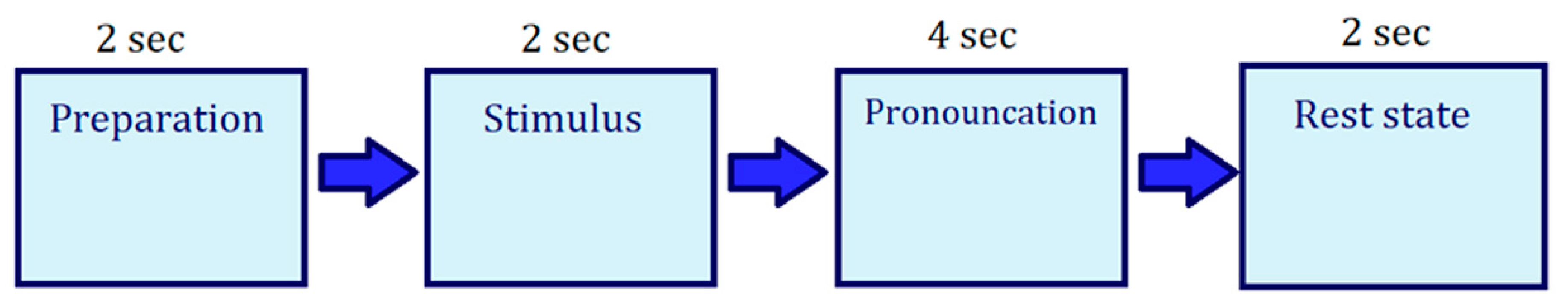
The dataset used in this study is recorded by Coretto et al. [19] in the Faculty of Engineering at the National University of Entre Ríos (UNER). Fifteen subjects performed overt and covert speech tasks, while their EEG signals were recorded. The data consist of trials in which the subjects had to pronounce the five main vowels “a”, “e”, “i”, “o”, and “u” and the six Spanish words corresponding to the English words for “up”, “down”, “left”, “right”, “back”, and “forward”, although the word part of the dataset is not used in this study. The EEG signals were recorded with an 18-channel Grass analogue amplifier and were sampled at 1024 Hz. The electrodes were positioned according to the 10–20 international system at positions F3, F4, C3, C4, P3, and P4, as shown in Figure 1. The experimental protocol for pronouncing the vowels and words had a two second pre-trial period where the subjects were shown their target. Following that there was a four second period during which the imagined pronunciation of the target took place. The vowel had to be pronounced during the whole four seconds, while the word was pronounced three times during the four second period. After that, there was a two second rest period. The protocol is illustrated on Figure 2. Only the vowel part of this dataset was used in this study.
The following section describes the methodology for replicating the results of the two chosen previous imagined speech classification attempts made on the same dataset. The first replication is an initial classification attempt by the collectors who collect the datasets and authors of the dataset themselves [19], and the second replication is done by Cooney et al. [8], where a CNN with 32 layers was used.
3.2. Validating and Verifying the Existing Studies
3.2.1. Replication of the First Study
The first replication is done on the results achieved by the same people who collected the data and made the dataset used in this study [19]. They used a random forest classifier to classify both the words and vowels of the dataset. They downscaled the data eight times and got an effective sampling rate of 128 Hz. After that, they computed a discrete wavelet transform (DWT) with five levels of decomposition for each EEG channel by selecting the mother wavelets from the Daubechies family. After that, they calculated the relative wavelet energy (RWE) for each channel in each sample and used the RWE for each decomposition, except for the first to form the feature vector with which to classify samples. A short guide on how to do this in Python is given here (http://ataspinar.com/2018/12/21/a-guide-for-using-the-wavelet-transform-in-machine-learning/).
Like the target paper, the first decomposition (corresponding to frequency bands 32–64) was not used in calculating the RWE. Wavelet transform and decomposition were implemented in Python using the “Pywt” library, which is a publicly available tool for implementing and using wavelet transform in Python. The experiment and random forest classifier training was conducted using a publicly available machine learning and feature analysis tool Weka. A random forest classifier made of 100 trees with five randomly chosen attributes was used to classify the data. The classifier used 10-fold cross validation and was trained 10 times.
3.2.2. Replication of the Second Study
The second replication is based on a study made by Cooney et al. [8] on the same dataset used in this study and by the study replicated in the previous section. They used a deep CNN with 32 layers to classify the vowels. Down-sampling, artefact removal, and data scaling were used as part of the pre-processing.
The CNN used is divided into seven sections, where the first section is the initial convolution part. This part contains the input layer as well as two initial convolution layers, the first being temporal convolution and the second being spatial convolution. The following five sections are all very similar convolution sections consisting of five layers each. The final section is the classification section, which has the softmax activation layer for classification. All of Cooney’s research was implemented in Python using Tensorflow and Keras libraries.
The pre-processing started with down-sampling the data to 128 Hz. FastICA was used for artefact removal on trials marked by the dataset authors as having artefacts and scikit-learn’s robust scaler was used for scaling the data. The data were shuffled prior to feeding them to the network. These data were then given to the 32-layer constructed CNN. All the details except for the pooling layers are provided by Cooney et al. [21]. The parameters of the pooling layers were selected to be the same as Schirrmeister et al. [23], the same CNN that inspired Cooney. Five-fold cross-validation was used and the best model from each fold was used to acquire the testing accuracy. All the folds were trained for 100 epochs, and a callback was used to stop the training when the validation loss had not improved for 50 epochs, which helps to reduce overfitting.
3.3. Proposed Model
Below is a description of all the parts of the CNN model proposed by this study. CNN was chosen as the architecture for the model because CNNs have become more popular in the recent years [9] and they have been shown to perform the best when faced with raw EEG data.
3.3.1. Pre-Processing
For the CNN, multiple pre-processing techniques were tried and, because the imagined speech data are recorded at a very high sample rate, down-sampling is safe to use. Data were down-sampled eight times down to 128 Hz and data were restructured from a simple array to a 2D array, where each element was stored as an array of the signal values at that time point. For vowels, all classes were balanced to the lowest class count on any subject of any trial type, which was 37 examples for subject 07 on “e”. No artefact removal was used because the intention of this study is to keep the overall model as simple as possible. Artefact removal is usually done manually and, as such, it requires a lot of extra work. Furthermore, the review by Roy [9] shows that 47% of studies do not use artefact handling, while only 23% do use it. It is suggested that using deep neural networks might be a way to avoid the artefact removal step. Additionally, only about 20% of the data have any artefacts in it. The data were split into three parts: 70% training data, 15% validation data, and 15% testing data.
3.3.2. Convolutional Neural Network
The most important aspects of a CNN are the number of layers and of which layers the CNN is made. While deeper neural networks may seem better on a first glance, a high number of layers has drawbacks in classification performance. They take longer to train and are more prone to overfitting. In addition, as Roy [9] noted in their review, shallower neural networks in some cases actually had better classification performance than deeper networks, and sometimes the best model was one with the number of layers somewhere in the middle. It is not clear whether shallow or deep models are better in all cases. When it comes to layer configuration then, for EEG, it is recommended that the model processes temporal and spatial information separately [9]. This is also investigated in this study.
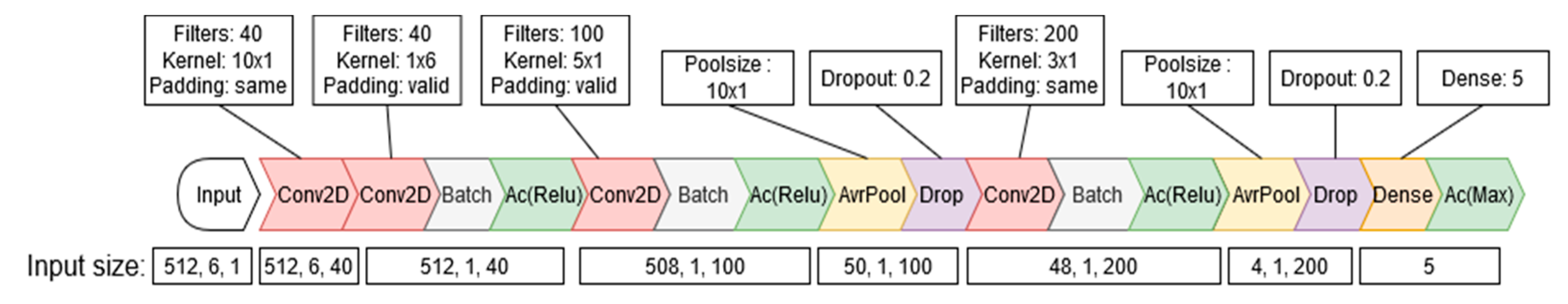
The neural network proposed in this study was inspired by the one proposed by Schirrmeister et al. [23]. This neural network consists of an initial convolution block followed by several separately viewable convolution blocks. The goal of this study is to reduce the complexity of the model and keep the number of considerably lower than in previous works to see if a simpler model with less number of layers can still perform imagined speech classification at an optimal level. Figure 3 describes all of the layers along with their parameters. The first block consists of an input layer, which is immediately followed by two 2D convolutional layers, one for temporal and one for spatial convolution, as well as a batch normalization and Relu activation layers. Following that, there are two identical convolution blocks, both of them consisting of the following: 2D convolution, batch normalization, Relu activation, average pooling, and dropout. The final classification part consists of a dense layer followed by a softmax classification layer. The model was implemented in Python with Keras and Tensorflow frameworks.
3.3.3. Training
The training of the models took place on the servers of the High Performance Computing Centre of Tartu University on the Rocket Clusters’ Falcon GPU nodes. The servers are made of 135 CPU nodes and 3 GPU nodes specifically made for machine learning. GPU nodes have two 24 core CPUs and 512 GB of RAM and eight NVIDIA Tesla P100 GPUs. The specific training server details can be found here (https://hpc.ut.ee/rocket-cluster/). Several callbacks were also used to select only the model with the highest validation accuracy. All three CNNs were trained with the Adam optimizer and sparse categorical cross entropy loss function. Adam optimizer works well in practice and compares favorably to other adaptive optimizers [24]. A learning rate of 0.001 was also recommended to be used with the Adam optimizer. The initial CNN was trained for 100 epochs. Early stopping was also in place to stop training if the validation accuracy did not improve in 50 epochs in order to stop overfitting.
3.3.4. Transfer Learning
Three TL approaches were used with the proposed model to try and improve the accuracy of the model. TL is a machine learning technique that aims to improve classification accuracy on a single subject. TL allows knowledge gained from training one network to be transferred to another, more specific network. For example, a model that is trained on 10,000 different cars can then be further retrained to be more focused on classifying trucks.
The three TL methods are described below. Different TL methods are used to find if fine-tuning the earlier layers or latter layers gives the best improvement when it comes to EEG tasks. TL is used to improve accuracies here as it was used in the comparison study [8] to confirm the effectiveness of TL on EEG data. All methods first train a model with the data from all subjects but one, and then use the combined weights to specifically optimise the model for that one subject by fine tuning some or all of the convolutional layers with that one person’s data. TL training sessions were 40 epochs long.
Transfer Learning Method 1
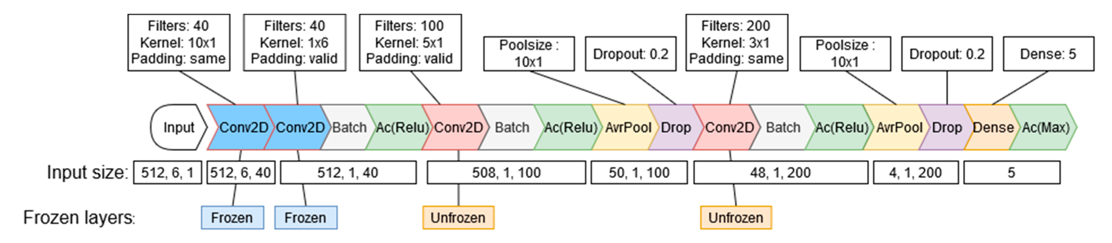
The first TL method freezes the whole base model and then unfreezes the first two convolutional layers to be retrained on the new subject’s data. This method locks all weights on the pre-trained network and allows only the first two convolutional layers to change when the network gets fine-tuned with data from S01. The three TL methods are illustrated on Figure 4, Figure 5, and Figure 6, respectively.
Transfer Learning Method 2
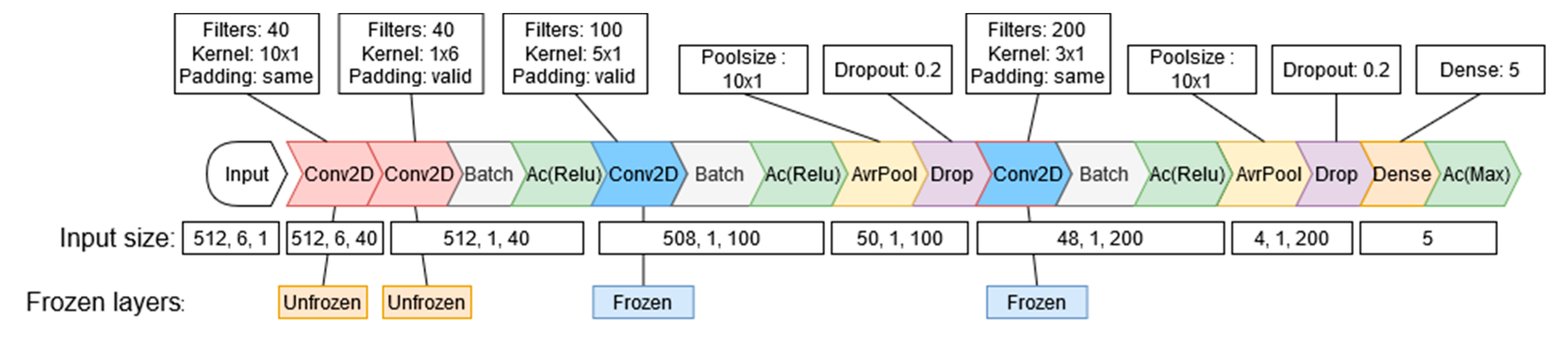
The second TL method freezes the whole base model and then unfreezes the last two convolutional layers to be retrained on the new subject’s data.
Transfer Learning Method 3
The third TL method uses a combination of both previous methods to try and unfreeze all of the convolutional layers to retrain on new subject data.
4. Results
In this section, we report the classification results we got for both the replicated and the proposed model. First are the results for the replication, and then the results for our new proposed convolution model and all of the TL methods.
4.1. Replication Results of the First Study
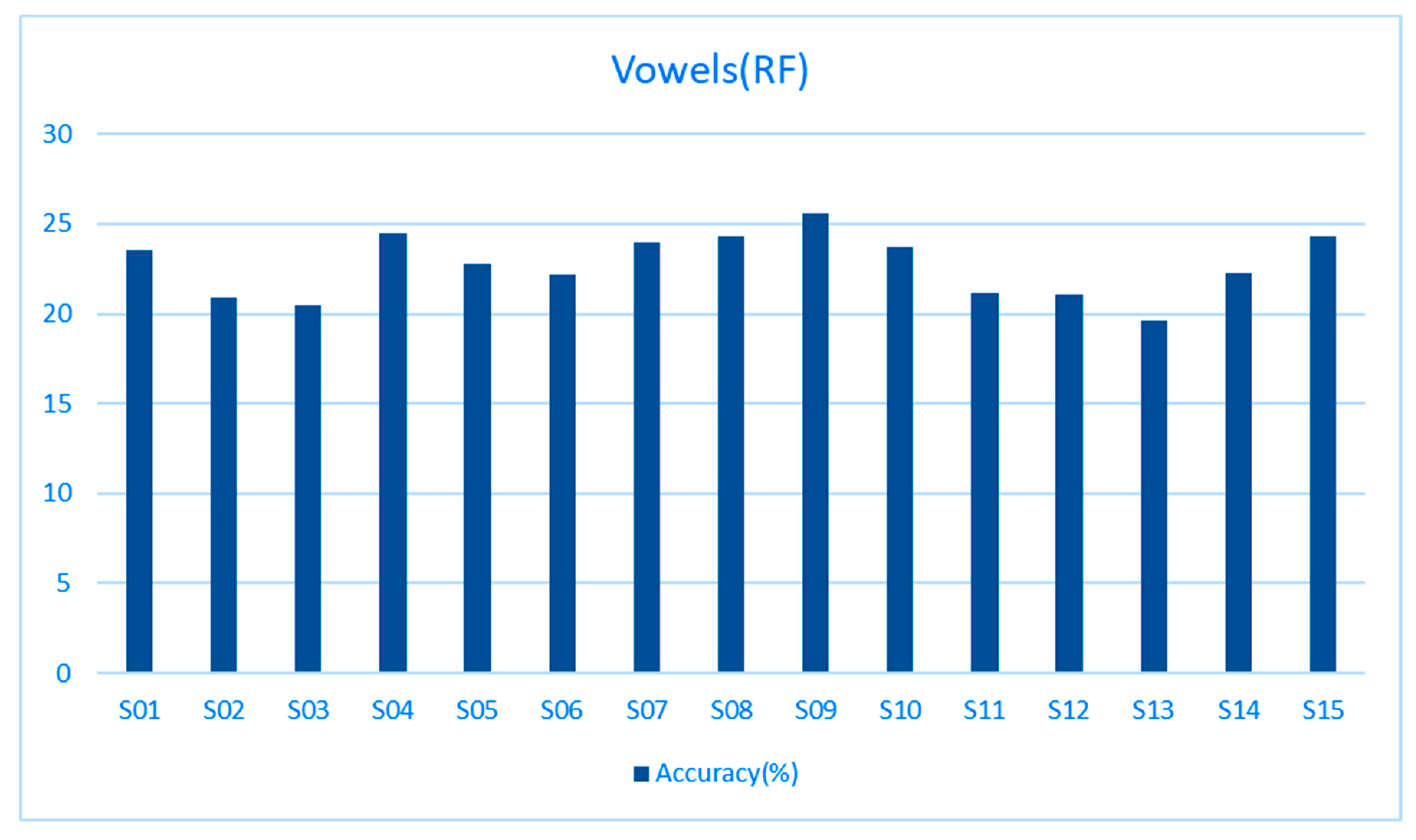
The first replication was done on the study by the authors of the dataset used in this study [19]. The mean accuracies for all subjects are presented in Figure 7. The mean accuracy over all subjects over 10 iterations with different seeds was 22.81%, which is just slightly above the first study’s mean accuracy. All of the subjects except S13 got a mean accuracy above the chance level (20%). The random seed numbers used by the authors of the first study are not brought out in that paper, so the random seeds used here are probably different than the ones used there and cause slightly different results.
4.2. Replication Results of the Second Study
The second replication was done on the study by Cooney et al. [8]. The mean accuracies for all subjects are presented in Figure 8. The mean accuracy over all subjects was 30.21%. This is considerably lower than the mean accuracy achieved by the authors (32.75%). This can be explained by the different artefact removal technique used and also possibly by different parameters used in the pooling layers, as those are not clearly defined in the second study. Different implementation platforms may also slightly influence accuracies. Accuracy is the mean test accuracy of the fivefold cross validation.
4.3. Results of the Proposed Model
The mean accuracies for the CNN and all of the TL methods are presented in Table 1 below. The proposed CNN with 16 layers managed to beat the random forest classifier (23.98% vs. 22.72%), which is presented in Table 1, which was used by the initial makers of the dataset, but it did not beat the significantly deeper and more complex neural network proposed by Cooney et al. on this same dataset (23.98% vs. 32.75%), which is presented in Table 1. However, the proposed model in this study is less complex, uses less data (class balancing), and also does not use the time-intensive artefact removal. Out of all the TL methods, the best results were achieved by the first TL method, as was the case in Cooney’s study [8].
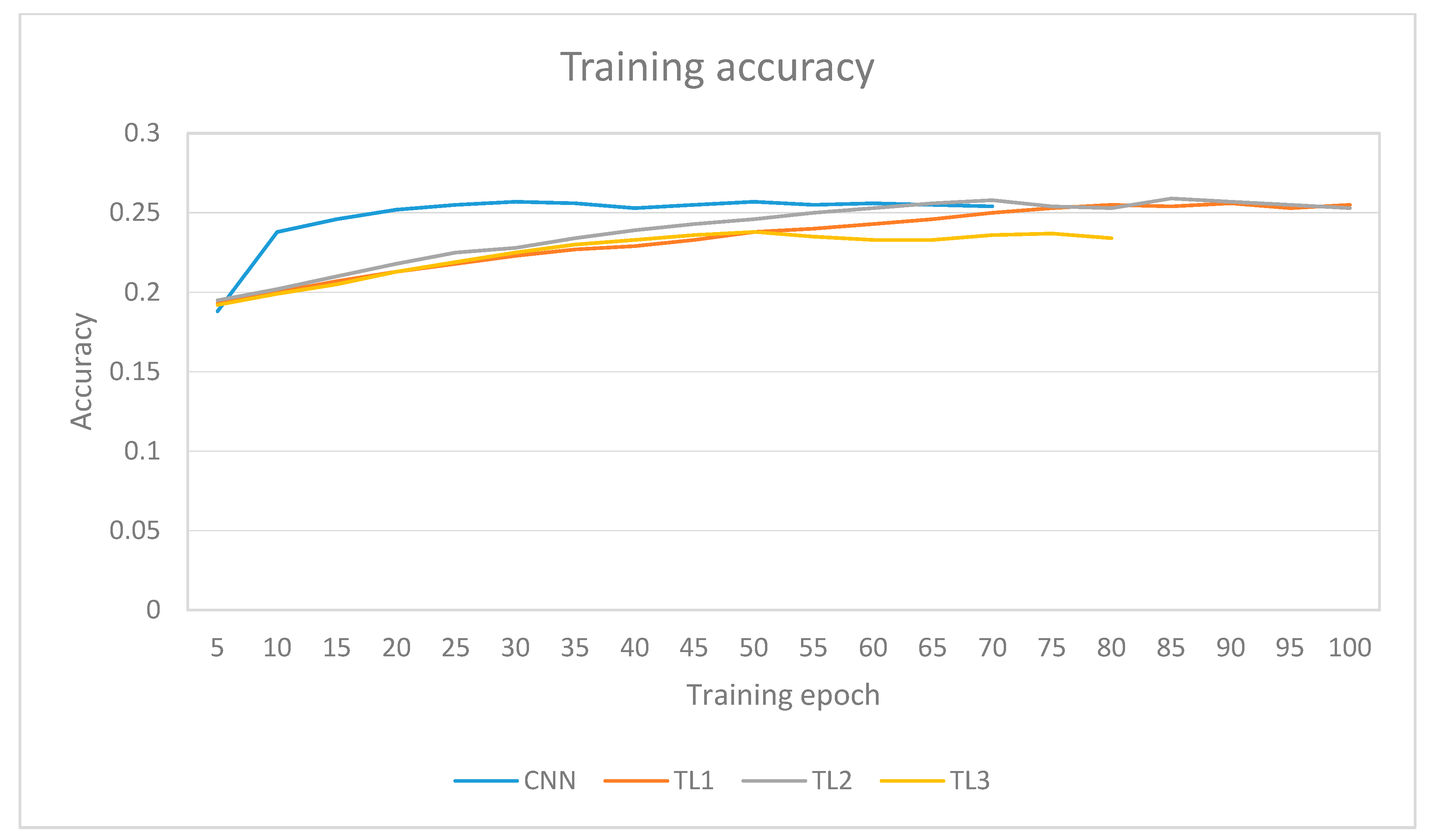
The training accuracy change over time can be seen in Figure 9, where the training accuracies for all of the models over their 100 epoch training period are depicted. The CNN and TL all three (TL1, TL2, and TL3) implemented methods in the proposed models stopped early owing to their validation accuracy not improving over 50 epochs. The CNN and TL of all three methods (TL1, TL2, and TL3) training accuracies quickly reached a plateau after training for about 20–30 epochs, and then stayed quite stable. TL1 and TL2 methods on the other hand trained a bit slower, but continued to improve a bit even in the later stages of the training.
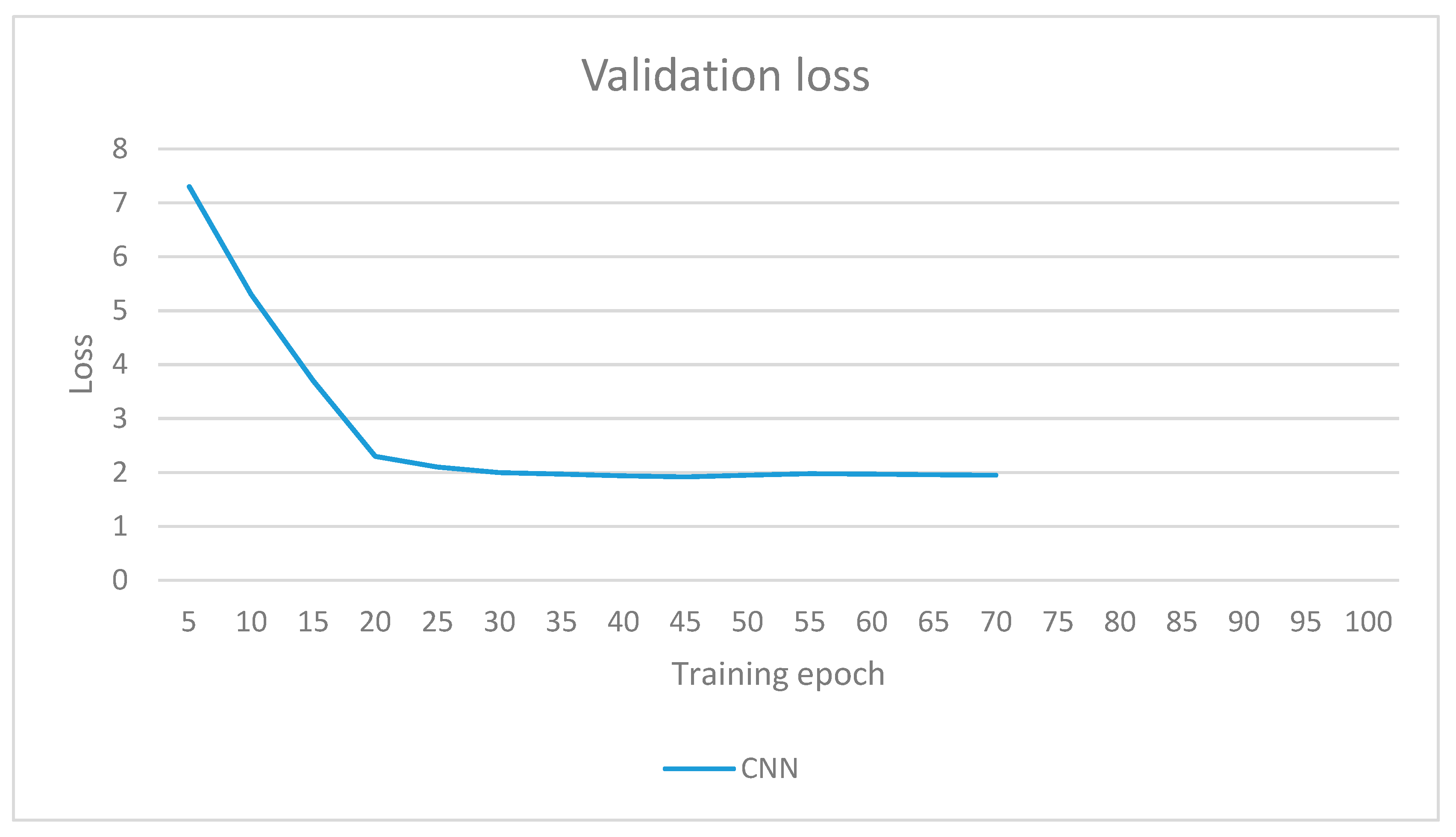
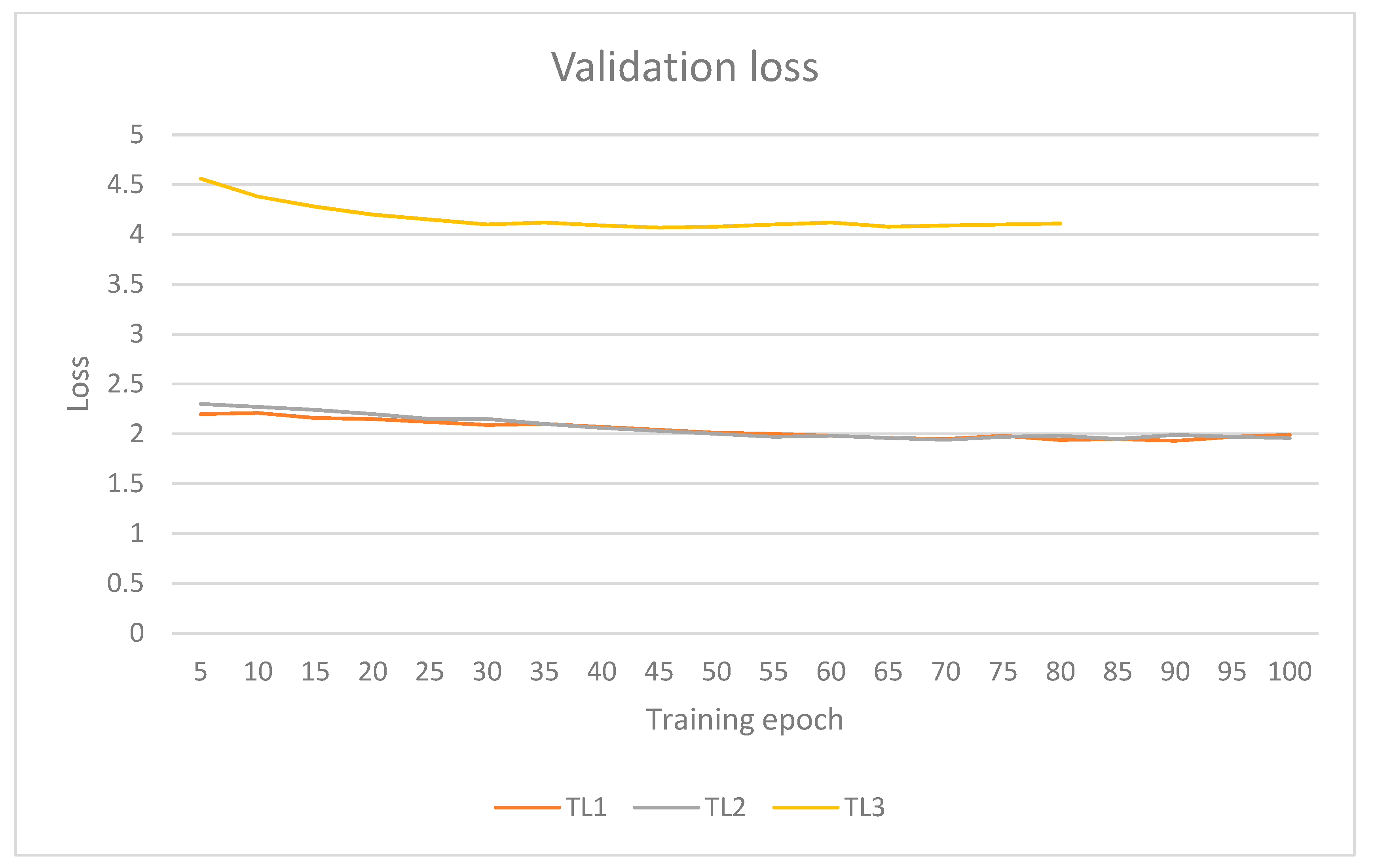
Validation losses for all models are presented in Figure 10 and Figure 11. The validation loss for the CNN (without TL) is presented in a separate figure as it had a great initial loss that was on a different scale to the TL methods. Validation loss for the non-TL model plateaued at around 2, while the TL1 and TL2 methods managed to have some epochs reach 1.93. TL3, on the other hand, started at a loss of 4.6, and its best epoch reached a loss of 4.1. Here, again, CNN and TL3 methods stopped early owing to their validation loss plateauing at around 20 to 30 training epochs. TL3 method had a much greater loss validation loss over other TL methods, which is an indication that this model does not generalise very well.
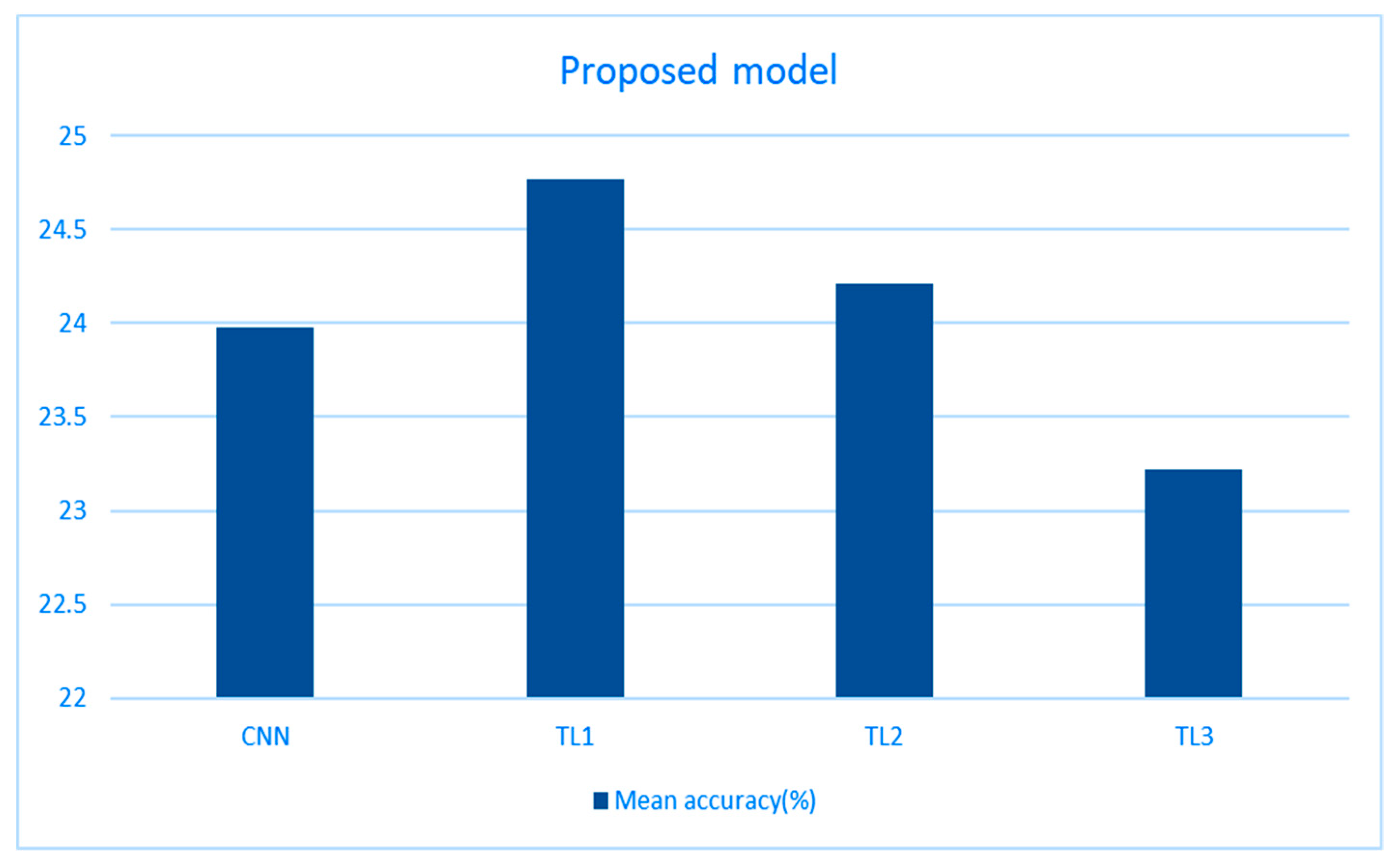
Figure 12 gives an overview of how well TL methods performed when compared with not using any TL methods. TL improved the accuracy in two out of three cases. The biggest improvement was seen when the fine-tuning took place on the initial convolutional layers and a considerable improvement was also seen when fine-tuning the latter layer. Using TL on all layers lowered the overall accuracy.
TL improved the accuracy in two out of three cases. The biggest improvement was seen when the fine-tuning took place on the initial convolutional layers and a slight improvement was also seen when fine-tuning the latter layer. Using TL on all layers lowered the overall accuracy.
The accuracies achieved by the proposed model are underwhelming when compared with those achieved by Cooney’s 32-layer CNN, but in their case, the network requires significant pre-processing, and their model has double the amount of layers and also uses more data because they do not do class balancing, as is done in this study.
5. Discussion
Replication provided very similar results in the first replicated study and considerably lower results in the second replicated study, but that can be attributed to slightly differing tools and methods used in the replication. The proposed model was moderately successful, but definitely underperformed when compared with a more complex model, but the proposed model is less complex and much simpler.
5.1. Replicated Results
The overall mean accuracy from the first replication of study is very similar to the result achieved in this study. The overall accuracies differ by only 0.09%. Accuracies between other subjects differ more. For example, the replicated papers’ best individual accuracy was achieved on subject S14, but in this case, was achieved on subject S09. The lowest accuracy was achieved on S12 on the replicated paper’s case and S13 in this case. These differences can be attributed to the fact that the replicated paper did not specifically mention the seed numbers used in training their RF classifier. These numbers were guessed when replication took place and most probably differ from the ones chosen in the original work. Overall, the replication results confirmed the results of previous studies.
The overall mean accuracies between the second study of replication differ a bit more—30.21% versus 32.75%, representing significantly worse results. The main difference between this and the replicated study is that a different artefact removal technique was used to remove artefacts from data. In the replication, artefact removal was used only on the trials marked by the authors of the dataset. The second study does not mention if they used artefact removal on all of the trials or only on the ones marked by the dataset authors themselves. Twenty percent of the samples in this dataset are marked by the creators to contain artefacts. It is possible that some of the non-marked samples might also contain artefacts, in which case Cooney’s artefact handling took care of those artefacts and, in this study, they stayed in the data, which also can influence the overall accuracy.
5.2. Results of the Proposed Model
The overall mean accuracy achieved over all subjects with the new model is 23.98%, which is above the chance line (randomly guessing) of 20.00% and is better than the accuracy from the first replication study (22.72%), but is a lot lower than the results from the second replication study (32.75%).
The TL methods helped slightly to increase the accuracy, but still did not manage to achieve desirable results. This all indicates that classifying EEG data takes quite a bit of effort, as EEG data are highly personalized, and the same imagined action gives off different signals when it is measured from different people. This could mean that using neural networks with a small amount of layers to classify EEG data could be an impossible task and deeper networks are to be preferred at least when it comes to classifying imagined speech data.
One reason for generally low accuracies across the board could be that this is a relatively high class-count classification task with a very limited amount of data acquired from quite a high number of subjects. This data scarcity was further amplified when the class balance took place. Machine learning models need a lot of data per class to learn the specific features relevant to each class and this dataset has a relatively small sample size to provide it. The low accuracies achieved in this study as well as previous studies on this dataset could also be indicative of the poor quality of the dataset, where the relevant features are not easily accessible for the classifiers. Perhaps the recording protocol could be optimised to have larger pauses between experiments and trials, as they have been shown to give better data [25].
The proposed CNN is much less complex than the previously designed model and takes considerably less knowledge and skills of machine learning to correctly implement on a variety of platforms. Artefact removal is a manual task and it takes a great understanding of EEG signals to correctly remove the irrelevant components during the removal process. If the amount of data is high, then this process can also take a long time. As such, our proposed model, although it is considerably less accurate, can be used in cases where the artefact handling proves to be too difficult to manually handle. As the neural network is also half the depth of the previous work, the model takes a lot less time to train and is useful when there is no access to high-performance computing equipment, as it can be trained faster than other models.
6. Conclusions and Future Work
First, the results of two different previous studies on the same dataset were replicated and confirmed. This dataset, which contains the imagined speech data from 15 subjects, was used to train our own classifier, which was then used to classify the imagined speech data. Three different TL methods were tried to improve the accuracy of the model. The first method fine-tuned the first two convolutional layers, the second fine-tuned the latter layers and the third tried to improve all convolutional layers.
The replication results were very similar to those achieved by the original authors. The dataset paper used a random forest classifier to classify both words and vowels. The replication achieved very similar results in vowels (22.81% vs. 22.72%). For the Cooney’s results the accuracies slightly differed (30.21% vs. 32.75%), but this can be explained with using a different artefact removal technique that was native to the platform that was used to implement the CNN. After the replication, a new CNN was constructed to try to achieve similar results to the previously implemented studies, but this time only using a 16-layer neural network. Different TL techniques were also tried. Achieved accuracies for the CNN (23.98%) and all three TL methods (24.77%, 24.12%, 23.22%) were better than that achieved by the authors of this dataset (22.72%), but fell short of that achieved by a considerably deeper network.
In the discussion, it was argued that, when it comes to classifying the highly personalised EEG imagined speech data, deeper neural networks should be used and additional data generation could prove very useful in improving the performance of the classifiers. TL in neural networks also showed promise and should be used in the future to help get better accuracies. It was shown that TL improved the classification accuracy the most when it was applied to the earlier layers of the neural network.
In the future, when it comes to using EEG data in imagined speech classification, it is recommended that, if the amount of data is low, then models with a high number of layers should be used or some additional data generation should be used to generate better classification accuracies. TL showed potential and its effect on both shallow and deep neural networks, as well as in the cases of a low and high amount of data, could be further explored.
Author Contributions
Conceptualization, M.-O.T., Y.M. and N.M.; Formal analysis, M.-O.T., Y.M. and N.M.; Investigation, M.-O.T., Y.M. and N.M.; Methodology, M.-O.T., Y.M. and N.M.; Software, M.-O.T., Y.M. and N.M.; Supervision, Y.M.; Validation, M.-O.T. and Y.M.; Visualization, M.-O.T., Y.M. and N.M.; Writing―original draft, M.-O.T.; Writing―review & editing, Y.M. and N.M. All authors have read and agreed to the published version of the manuscript.
Funding
This research received no external funding.
Acknowledgments
Naveed Muhammad has been funded by European Social Fund via IT Academy programme.
Conflicts of Interest
The authors declare no conflicts of interest.
References
- Edelman, B.J.; Meng, J.; Suma, D.; Zurn, C.; Nagarajan, E.; Baxter, B.S.; Cline, C.C.; He, B. Noninvasive neuroimaging enhances continuous neural tracking for robotic device control. Sci. Robot. 2019, 4. [Google Scholar] [CrossRef] [PubMed]
- Anumanchipalli, G.K.; Chartier, J.; Chang, E.F. Speech synthesis from neural decoding of spoken sentences. Nature 2019, 568, 493–498. [Google Scholar] [CrossRef] [PubMed]
- Ramadan, R.A.; Vasilakos, A.V. Brain computer interface: Control signals review. Neuroscience 2017, 223, 26–44. [Google Scholar] [CrossRef]
- Puce, A.; Hämäläinen, M.S. A review of issues related to data acquisition and analysis in EEG/MEG studies. Brain Sci. 2017, 7, 58. [Google Scholar] [CrossRef] [PubMed]
- Bogue, R. Brain-computer interfaces: Control by thought. Ind. Robot. Int. J. 2010, 37, 126–132. [Google Scholar] [CrossRef]
- Cooney, C.; Folli, R.; Coyle, D. Mel Frequency Cepstral Coefficients Enhance Imagined Speech Decoding Accuracy from EEG. In Proceedings of the 29th Irish Signals and Systems Conference (ISSC), Belfast, UK, 21–22 June 2018. [Google Scholar]
- Chen, W.; Wang, Y.; Cao, G.; Chen, G.; Gu, Q. A random forest model based classification scheme for neonatal amplitude-integrated EEG. Biomed. Eng. Online 2014, 13. [Google Scholar] [CrossRef] [PubMed] [Green Version]
- Cooney, C.; Raffaella, F.; Coyle, D. Optimizing Input Layers Improves CNN Generalization and Transfer Learning for Imagined Speech Decoding from EEG. In Proceedings of the IEEE International Conference on Systems, Man, and Cybernetics, Bari, Italy, 6–9 October 2019. [Google Scholar]
- Roy, Y.; Banville, H.; Albuquerque, I.; Gramfort, A.; Falk, T.H.; Faubert, J. Deep learning-based electroencephalography analysis: A systematic review. J. Neural Eng. 2019, 16. [Google Scholar] [CrossRef] [PubMed]
- Song, Y.; Sepulveda, F. Classifying speech related vs. idle state towards onset detection in brain-computer interfaces overt, inhibited overt, and covert speech sound production vs. idle state. In Proceedings of the 2014 IEEE Biomedical Circuits and Systems Conference (BioCAS), Lausanne, Switzerland, 22–24 October 2014. [Google Scholar]
- Zhao, S.; Rudzicz, F. Classifying phonological categories in imagined and articulated speech. In Proceedings of the 2015 IEEE International Conference on Acoustics, Speech and Signal Processing (ICASSP), Brisbane, Australia, 19–24 April 2015. [Google Scholar]
- DaSalla, C.S.; Kambara, H.; Sato, M.; Koike, Y. Single-trial classification of vowel speech imagery using common spatial patterns. Neural Netw. 2009, 22, 1334–1339. [Google Scholar] [CrossRef] [PubMed]
- Brigham, K.; Kumar, B.V.K.V. Imagined Speech Classification with EEG Signals for Silent Communication: A Preliminary Investigation into Synthetic Telepathy. In Proceedings of the 2010 4th International Conference on Bioinformatics and Biomedical Engineering, Chengdu, China, 18–20 June 2010. [Google Scholar]
- Yang, B.; Duan, K.; Fan, C.; Hu, C.; Wang, J. Automatic ocular artifacts removal in EEG using deep learning. Biomed. Signal Process. Control. 2018, 43, 148–158. [Google Scholar] [CrossRef]
- Moctezuma, L.A.; Molinas, M.; Torres-García, A.A.; Villaseñor-Pineda, L. Towards an API for EEG-Based Imagined Speech classification. In Proceedings of the International conference on Time Series and Forecasting, Granada, Spain, 19–21 September 2018. [Google Scholar]
- Chi, X.; Hagedorn, J.B.; Schoonover, D.; D'Zmura, M. EEG-Based discrimination of imagined speech phonemes. Int. J. Bioelectromagn. 2011, 13, 201–206. [Google Scholar]
- Amin, S.U.; Alsulaiman, M.; Muhammad, G.; Mekhtiche, M.A.; Hossain, M.S. Deep Learning for EEG motor imagery classification based on multi-layer CNNs feature fusion. Futur. Gener. Comput. Syst. 2019, 101, 542–554. [Google Scholar] [CrossRef]
- Waytowich, N.; Lawhern, V.J.; Garcia, J.O.; Cummings, J.; Faller, J.; Sajda, P.; Vettel, J.M. Compact convolutional neural networks for classification of asynchronous steady-state visual evoked potentials. J. Neural Eng. 2018, 15. [Google Scholar] [CrossRef] [PubMed]
- Coretto, G.A.P.; Gareis, I.; Rufiner, H.L. Open access database of EEG signals recorded during imagined speech. In Proceedings of the 12th International Symposium on Medical Information Processing and Analysis, Tandil, Argentina, 1 January 2017. [Google Scholar]
- García-Salinas, J.S.; Villaseñor-Pineda, L.; Reyes-García, C.A.; Torres-García, A. Tensor decomposition for imagined speech discrimination in EEG. In Advances in Computational Intelligence. MICAI 2018; Springer International Publishing: Guadalajara, Mexico, 2018. [Google Scholar]
- Cooney, C.; Korik, A.; Raffaella, F.; Coyle, D. Classification of imagined spoken word-pairs using convolutional neural networks. In Proceedings of the 8th Graz Brain Computer Interface Conference 2019, Graz, Austria, 16–20 September 2019. [Google Scholar]
- Tan, P.; Sa, W.; Yu, L. Applying extreme learning machine to classification of EEG BCI. In Proceedings of the 2016 IEEE International Conference on Cyber Technology in Automation, Control, and Intelligent Systems (CYBER), Chengdu, China, 19–22 June 2016. [Google Scholar]
- Schirrmeister, R.T.; Springenberg, J.T.; Fiederer, L.D.J.; Glasstetter, M.; Eggensperger, K.; Tangermann, M.; Hutter, F.; Burgard, W.; Ball, T. Deep learning with convolutional neural networks for EEG decoding and visualization. Hum. Brain Mapp. 2017, 38, 5391–5420. [Google Scholar] [CrossRef] [PubMed] [Green Version]
- Ruder, S. An overview of gradient descent optimization algorithms. arXiv 2016, arXiv:1609.04747. [Google Scholar]
- Muhammad, Y.; Vaino, D. Controlling Electronic Devices with brain rhythms/electrical activity using artificial neural network (ANN). Bioengineering 2019, 6, 46. [Google Scholar] [CrossRef] [PubMed] [Green Version]
Figure 1.
10–20 international electrode positioning (https://en.wikipedia.org/wiki/10%E2%80%9320_system_(EEG)); data are acquired from highlighted electrodes.
Figure 1.
10–20 international electrode positioning (https://en.wikipedia.org/wiki/10%E2%80%9320_system_(EEG)); data are acquired from highlighted electrodes.

Figure 2.
Recording protocol used to collect data from subjects.

Figure 3.
The proposed model’s layers and their parameters.

Figure 4.
Transfer learning (TL) method 1: initial layers are frozen.

Figure 5.
Transfer learning method 2: latter layers are frozen.

Figure 6.
TL method 3: all layers are unfrozen.

Figure 7.
First study replication results per subject. RF, random forest.

Figure 8.
Second study replication results per subject. CNN, convolutional neural network.

Figure 9.
Training accuracy over time for all models.

Figure 10.
Validation loss over time for the non-TL method.

Figure 11.
Validation loss over time for TL methods.

Figure 12.
Comparison of different TL methods used on the proposed model.


Table 1.
Comparison between accuracies of replicated studies and the proposed model.
| First Replicated Study | Second Replicated Study | Proposed Model | |
|---|---|---|---|
| Accuracy | 22.72% (±1.81) | 32.75% (±3.23) | 23.98% (±3.08) |
| Replication | 22.81% (±1.93) | 30.21% (±3.94) | --- |
© 2020 by the authors. Licensee MDPI, Basel, Switzerland. This article is an open access article distributed under the terms and conditions of the Creative Commons Attribution (CC BY) license (http://creativecommons.org/licenses/by/4.0/).
Share and Cite
MDPI and ACS Style
Tamm, M.-O.; Muhammad, Y.; Muhammad, N. Classification of Vowels from Imagined Speech with Convolutional Neural Networks. Computers 2020, 9, 46. https://0-doi-org.brum.beds.ac.uk/10.3390/computers9020046
AMA Style
Tamm M-O, Muhammad Y, Muhammad N. Classification of Vowels from Imagined Speech with Convolutional Neural Networks. Computers. 2020; 9(2):46. https://0-doi-org.brum.beds.ac.uk/10.3390/computers9020046
Chicago/Turabian StyleTamm, Markus-Oliver, Yar Muhammad, and Naveed Muhammad. 2020. "Classification of Vowels from Imagined Speech with Convolutional Neural Networks" Computers 9, no. 2: 46. https://0-doi-org.brum.beds.ac.uk/10.3390/computers9020046
Note that from the first issue of 2016, this journal uses article numbers instead of page numbers. See further details here.