An UML Based Performance Evaluation of Real-Time Systems Using Timed Petri Net


1
Department of Computer Science and Engineering, Manipal Institute of Technology, Manipal Academy of Higher Education, Manipal 576104, India
2
Software Consultant, Manipal 576104, India
*
Author to whom correspondence should be addressed.
Computers 2020, 9(4), 94; https://0-doi-org.brum.beds.ac.uk/10.3390/computers9040094
Submission received: 23 October 2020
/
Revised: 17 November 2020
/
Accepted: 24 November 2020
/
Published: 27 November 2020
Abstract
:Performance is a critical non-functional parameter for real-time systems and performance analysis is an important task making it more challenging for complex real-time systems. Mostly performance analysis is performed after the system development but an early stage analysis and validation of performance using system models can improve the system quality. In this paper, we present an early stage automated performance evaluation methodology to analyse system performance using the UML sequence diagram model annotated with modeling and analysis of real-time and embedded systems (MARTE) profile. MARTE offers a performance domain sub-profile that is used for representing real-time system properties essential for performance evaluation. In this paper, a transformation technique and transformation rules are proposed to map the UML sequence diagram model into a Generalized Stochastic Timed Petri net model. All the transformation rules are implemented using a metamodel based approach and Atlas Transformation Language (ATL). A case study from the manufacturing domain a Kanban system is used for validating the proposed technique.
1. Introduction
Model-driven engineering (MDE) is considered a new paradigm in the field of Software Engineering where models play a vital role in system representation. MDE is proposed by Object Management Group (OMG) and it focuses on using models as main artifacts for understanding domain conceptual models for a specific problem. In MDE based system development, models can be used to model different system components and interaction between them, capturing the system behaviour. Particularly for a complex system, models can give an abstract view of the entire system and can be explored to analyze system functionality at an early stage of system development.
The Integration of system performance analysis and understanding system functionality at an initial stage of system development has gained popularity among researchers during recent times. During the initial stage of system development, Unified Modeling Language(UML) [1] is the standard modeling language used for system representation. UML is a semi-formal language that could be used for system presentation and analysis, even as an input to tools for further analysis and automated generation of software prototypes within computer-aided software engineering (CASE) tools. Integrating formal techniques and formal models with UML can lead to a path in achieving early stage system performance analysis using UML and formal models. Modeling real-time properties and performance analysis requirements are possible through UML supported real-time profiles.
In this paper, we adopt modeling and analysis of real-time and embedded systems (MARTE) [2] profile for extending UML model with real-time properties. There exist other works that propose the mapping of semi-formal models into formal models, such as Petri net [3,4,5,6], Queueing Petri net [7] and others [8,9].
The approach we propose here is motivated to influence the software development process with model-driven approach. The software industry focuses more on the programming approach to provide solutions for user requirements rather than modeling approaches. Currently, the impact of model-driven approach in the software industry is limited, as the adoption of model-driven approach could require a series of the social, organizational issue concerned with the management of changes as discussed in [10,11]. and also evaluate the outcome. but it can be improved by exposing the ability of formal models in modeling and analyzing the system during development. The model driven approaches can be implemented using model-driven transformation for mapping information’s from the input source model to target models. Considering the domain of software engineering, UML is the de-facto standard used for input models and the target models can be automatically generated using model transformation techniques. Some of the commonly used transformation languages in the literature are Atlas Transformation Language (ATL), Epsilon family (ETL), Kermata, Query view Transformation language (QVT) etc. [12,13,14].
In this paper, we use a UML sequence diagram as an input model to represent real-time system scenarios and Generalized Stochastic Petri net (GSPN) as the target model to study system behaviour. Generalized Stochastic Petri net is a Timed Petri net model with the mathematical background well suitable to be used as a performance model [15]. Generalized Stochastic Petri net is described with arcs and nodes represented as the transition to describe events occurring and places describing conditions within the system. Places and transitions are connected by directed arcs to define the flow of control(execution). GSPN includes two types of transition: timed transition and immediate transition [16]. Timed transitions include exponential distribution suitable to model random delay and immediate transitions suitable to model logical actions that do not consume time (zero delay). Since in real-time scenario all software activities do not require a probabilistic delay, GSPN is most suitable to model the real-time systems with activities associated with delay as well as zero delay.
An approach for integrating UML/MARTE models with the Generalized Stochastic Petri net model using Java and ATL transformation language is proposed in this paper. ATL is developed as a part of the ATLAS Model Management Architecture (AMMA) platform [17] and ATL is a metamodel based language that supports both metamodel syntax and textual concrete syntax. The proposed method will aid in improving design quality and eventually the system under development. The methodology uses a metamodel based approach to transform UML/MARTE model into the Generalized Stochastic Petri net model using Petri Net Markup Language (PNML) as the intermediate model. PNML is a standard interchange format used within the Petri net community to support the exchange of information between Petri net tools [18]. PNML intermediate model supports interoperability among different Petri net tools. The advantage of the PNML intermediate model is the flexibility to use the derived formal model with different Petri net tools and their functionalities. The proposed methodology is different in the way that it uses the existing models and metamodels rather than designing from scratch.
Earlier works have proposed mapping of UML models into Petri net models with transformation rules designed considering a specific kind of Petri net model and tool for analysis and hence does not provide a generalized approach to extend across different types of Petri net modeling tools. The main advantage of our paper is the transformation of UML model into a standard interchange format and its applicability across different types of Petri net modeling tools.
In summary, the proposed research implements a model-driven approach to transform UML/MARTE sequence diagram to the Generalized Stochastic Petri net model. The approach is implemented using Java and ATL transformation language. In the process of transformation, we define the following objectives.
- To design UML/MARTE based sequence diagram metamodel and PNML metamodel.
- To design and implement ATL transformation rules and automate the mapping of the UML/MARTE sequence diagram into PNML based GSPN.
- To verify the usability of the proposed methodology using a real-time system and analysing the system performance parameters.
The rest of the paper is organized as follows: Section 2 offers an overview of the state of the art, Section 3 provides an introduction to preliminaries, Section 4 provides an overview of methodology and transformation rules, Section 5 discusses an example on the manufacturing system and Section 6 provides concluding remarks and future work.
2. State of the Art
The proposed approach covers different aspects of research, such as use of model transformation languages, implementation of generalized representation of performance model, and use of UML profiles for performance evaluation. There exist other related works using UML models and performance models for an early stage performance evaluation of systems. These works include either of these three aspects mentioned above. These works are presented in the following order: Use of transformation languages (Section 2.1), use of UML profiles (Section 2.2), and other related works (Section 2.3).
2.1. State of the Art: Use of Transformation Languages
Li Dan [8] proposes a method for mapping sequence diagrams to Communication Sequential Processes (CSP). The mappings are designed and developed based on the standards, such as Meta Object facility (MOF), QVT, and Extensible Stylesheet Language Transformations (XSLT). This work uses a metamodel based approach and XSLT rule-based style templates are used for the mappings. For an XSLT engine, the input model is an XMI file of sequence diagram and then the XSLT engine executes the XSLT templates to produce an XML file of the CSP model. The target CSP model used in this work supports only verification of system properties in contrast to the Petri net used in our proposed work which can be used for both properties checking and quantitative performance analysis.
Elkamel Merah et al. [19] presents a meta model-based transformation approach to map UML sequence diagram to Petri net. The transformation approach is implemented using the Atlas Transformation Language (ATL). The paper proposes a set of ATL transformation rules for mapping a few sequence diagram elements into Petri net elements. This work considers the basic Petri net type and very few sequence diagram elements for transformation.
Joao Antonio Custodio Soares et al. [3] propose an automated approach of transforming the UML sequence diagram to Coloured Petri Nets (CPNs). CPN can be used as a formal model for future analysis. In this work, the author has used Epsilon Transformation Language to design transformation rules for mapping UML sequence diagram elements into the CPN model. This approach generates an end-to-end mapping from sequence diagram to CPN tool and hence does not provide a general format to be used across different Petri net tools and hence missing a unified approach.
Hassan Reza and Amrita Chatterjee [6] use Architecture Analysis and Design Language (AADL) for specification and verification of real-time embedded systems non functional properties. Since AADL lacks the formal semantics necessary to verify critical safety properties authors in this paper propose a method to supplement AADL with exiting formal methods and supporting tools for automatically verifying the critical system properties. The formal model used is Petri net and Petri Net Markup Language is used as a standard interface for different classes of Petri net. Hence, the author proposes an automated mapping of AADL elements into PNML elements using XSLT transformation techniques.
Yousra Ben Daly Hlaoui et al. [20] proposes a meta-model based transformation technique to specify and verify workflow applications of cloud services. The paper provides an approach for the reasoning of sequence diagram using the Event-B method. KerMeta transformation environment was used for the development of a tool using the proposed transformations.
It is observed that there exist works using specific transformation languages but most of the work support either the quantitative or qualitative analysis and lacks an automated approach for supporting both variants. Furthermore, the transformations are supported for only a few of the UML model elements, and specific to the output model format. Hence, there exists scope for more extensive transformation techniques with a unified approach.
2.2. State of the Art: Use of UML Profiles
S. Bernardi et al. in [21] proposes the Model-Driven approach for evaluating Reliability. Availability, Maintainability aspects of a real-time system. The author uses UML/MARTE profile and its extension dependability modeling and analysis (DAM) framework. The applicability of this approach is studied using the railway application. Model transformations using MARTE-DAM specifications are defined to generate Repairable Fault Tree and Bayesian Network models. This paper demonstrates the flexibility of the MARTE profile in extending its feature according to domain requirements. The approach shows only the transformation approach and lacks the result analysis to verify the transformation approach.
Davide Brugali [9] proposes an automatic approach for modeling and verification of non-functional properties of a robotic system. In this paper, the author has proposed an extension known as Autonomous Robot Modeling (ARM) profile to the UML/MARTE profile with robotic-specific non-functional requirements. The use of the proposed extension is discussed with a robot navigation system model. UML MARTE sequence diagram annotated with ARM is transformed into a Constraint Satisfaction Problem (CSP) model and non-functional requirements are verified.
J.I Requeno et al. [22] proposes a unique approach for modeling and performance analysis of real-time storm applications. The storm concepts are added as stereotypes into the UML MARTE profile. The author proposes transformation patterns for mapping UML activity and deployment diagrams and concepts into Generalized Stochastic Petri Nets for performance evaluation. The storm concepts are represented using customized stereotypes leading to the question of validity and acceptance level of these new stereotypes.
Vittorio Cortellessa et al. [23] proposes a bi-directional model transformation technique between UML state machines and GSPN model. The transformations are based upon the input UML state machine metamodel and the output GSPN metamodel. The paper focuses on the problems related to software availability. In our proposed method the transformation rules are designed for the input UML sequence diagram and output PNML metamodel. The obtained GSPN model in the proposed method is the standard form and hence it is possible to use the derived Petri net model across different Petri net tools. The interoperability across the different Petri net tools using the standard PNML format is a unique contribution of the proposed transformation technique. We have implemented a lightweight transformation technique using ATL and Java programming languages which does not require any additional software except Eclipse IDE.
Some of the works [24,25,26] have focused on transformation rules and their challenges involved in transforming UML annotated models into a specific performance analysis tool. In these works, GreatSPN is the tool used for analyzing the system performance. In [27], the authors provide the performance assessment of an industrial project INREDIS architecture using UML models and software performance evaluation (SPE) procedure. For the performance evaluation, ArgoSPE tool is used that generate GratSPN based GSPN model. In [28], uses a model-driven prediction method called Q-ImPrESS on a large-scale process control system from ABB Corporate Research to trade off the different architecture alternatives for determining the predicted performance accuracy, reliability prediction, and sensitivity analysis.
In summary few of the works have used the customized sub-profiles specific to their domain requirements and applications. The works also suggest that the MARTE profile can be extended accordingly. However, there exist very few works that use the existing MARTE sub-profiles for system performance evaluation, and hence we show the applicability of the existing MARTE profile and sub-profile. The proposed technique generates the output model in a standardized form which is missing in other works
2.3. State of Work: Other Related Works
Sebastian Ehmes et al. [29] proposes a general purpose tool for simulation of stochastic processes which can be used to study the scenarios in real-time systems. In this paper, the author uses a graph transformations for stochastic processes and it is possible to apply graph based approach for different domains that have stochastic processes.
Jieshi Shen et al. [5] offers a method to overcome the difficulty of analysis and verification of dynamic behaviour of the system using SysML state diagrams and formal Petri net. The authors transform state machines into the Petri net models for the study. Earlier studies focus on the one-to-one correspondence between SysML elements and Petri nets. Innovative investigation of the transition between two or more concurrent SysML state machines is suggested in this paper. The formal model used in this work is a basic Petri net and hence cannot support deeper performance analysis required for studying complex systems.
Federico Ciccozzi et al. in [30] proposes a systematic study and review of different works carried in the field of model-driven engineering and the use of UML models in system development. This paper particularly focuses on the execution of UML models and their contribution to developing an efficient system. The paper suggests that a lot of research is carried out in this field but still, there is a lot of scope in various aspects such as support execution of incomplete or partial UML models, solution for model-level debugging, less use of empirical methods. Hence, there exists scope for conducting research in model-driven engineering and add to the knowledge.
Jie Ding et al. [31] discovers the compositional structures of a given Petri net model. The paper proposes a sorting algorithm for analyzing the compositional structures of a Petri net model using an incidence matrix. The paper enhances the compositional analysis ability of Petri net. Large scale system is usually composed of complex compositional structures. Most of the modeling tools require composition and here the author proposes a method to identify the different possible composition structures of a Petri net model.
Vu Van Doc and Thang Huynh Quyet [32] discuss the transformation rules for mapping only a few sequence diagram elements and lack the rules for combined fragments such as “alt”, “par”, “loop” etc. The paper also does not provide the details of the transformation approach and any qualitative results of analyzing the derived Queueing Petri Net.
There also exist other commercial frameworks such as [33,34,35] that support the early stage modeling and performance evaluation of a system. However, most of these frameworks support only a specific analysis tool for example [34] uses Petri net as a formal model and derives the Petri net format specific for GreatSPN tool and hence it lacks a standard format of Petri net model. The DICE simulation tool proposed in [35] is close to our approach in a way that both approaches uses UML models as input and GSPN model as output and uses standard PNML format, gaining the possibility to use other Petri net analyzers. However, in DICE the input models are annotated with specially created DICE profile and are focused toward data intensive applications and Big-Data technology. As in our approach, we are using MARTE profile with annotation and stereotypes suitable for real-time and embedded systems. We have implemented a light weighted transformation techniques using ATL and Java programming languages and do not require any additional software.
In summary, most of the earlier works concentrate on a particular type of Petri net model and tool for transformations and do not provide a unified approach to support different Petri net tools into the MDE development approach. The main advantage of our approach is that it uses UML models extended with MARTE profile stereotypes and represents real-time system requirements and specifications which lacks in most of the earlier works. There exist very few works implementing quantitative evaluation of a system using UML models as considered in our work. Besides, our approach is the approach that implements a generalized intermediate PNML representation of the input model that is translated into a Petri net model for further evaluation using different Petri net tools. This offers an advantage to share the Petri net model across different users. Such interoperability is not possible using end-to-end transformation between a given type of input and output models as implemented in most of the earlier works.
3. Preliminaries
3.1. Timed Petri Net
In this section, we present the definition, theories, and analysis methods for Timed Petri nets used in subsequent parts of this paper. Detailed discussion is provided in [15,36].
Petri net is a mathematical modeling language used for discrete event-based distributed systems. It is graphically a directed graph with two types of nodes places and transition. Places are drawn as circles and transitions drawn as bars. These two nodes are connected with arc. Places can contain tokens, represented as back dots within places.
Petri net can be formally defined as N = (P, T, A, , W), where:
P = (, , …, ) is a finite set of places,
T = (, , …, ) is a finite set of transitions,
A ⊆ (P×T)∪(T×P) is a set of directed arcs, with each transition connected to at least one place.
For each transition t ∈ T we define input and output set of arcs as follows: →t = p∈P: {In(t,p)>0}, t→ = p∈P: {Out(p,t)>0}
- In(t) and Out(t), represents the multiset of input and output places of transition t, respectively
- In(t,p) and Out(p,t) represents the multiplicity of Place p in the multiset T(t)
: P→N is the initial marking function, that assigns to each place a natural number {0,1,2,…}. In the marking function, M(p) for p∈ P, is the number of tokens in place p in marking M,
W: F→ (1,2,…) defines a weight function to assign weights for arc.
The dynamics of the Petri net model is described by the changes in markings influenced by the transition firings. In timed Petri nets, each transition is associated with a random firing rate [37]. Transition firing results in an increase or decrease of tokens and it is governed by “enabling rule” and “firing rule” defined as follows:
Definition 1
(Enabling Rule). A transition t in Marking M is enabled if each of the input places of transition t is marked with at least W(p, t) tokens, where W(p, t) is the weight of the arc from p to t. Formally it is defined as:
Definition 2
(Firing Rule). A firing of a transition t in marking M creates a new marking M and removes W(p, t) tokens from all the input place of t, and adds W(t, p) tokens to each output place of transition t, where W(t, p) is the weight of the arc from t to p.
The firing rule defines the evolution of a Petri net model and creates a reachability set defined as follows:
Definition 3
(Reachability Set). The Reachability Set of a PN system with initial marking M is denoted RS(M), and is defined as a set of markings reachable from M.
Given a reachability set, we cannot get information about the sequence of transition firing to reach any marking. This information is provided by the reachability graph. In reachability, each node represents a reachable state and an arc from marking M to M if and only if the marking M is directly followed by M.
Petri net model supports various properties that can be verified or proved using several analysis techniques. The state space analysis or it is also known as reachability analysis is one such technique that can be used to study Petri net properties as well as to derive performance parameters [38]. Reachability analysis is based upon the initial marking and construction of a reachability graph of the Petri net.
In this paper, we derive performance parameters using the reachability set and reachability analysis technique.
3.2. MARTE Profile for Performance Modeling and Analysis
In this section, we describe briefly the MARTE profile required for the partial implementation of the first objective that involves designing UML/MARTE metamodel and also for designing the UML/MARTE sequence diagram of a system. MARTE is an extension of the UML standard to provide a mechanism for model-driven development of real-time and embedded systems. Such an extension can be used as an assistant for specification, design, verification, and validation stages of system development. MARTE profile is organized into two subsections: the MARTE design model and the MARTE analysis model. The former design model is used for modeling features of real-time and embedded systems and the latter is used for analysis purposes. MARTE model is very convenient as it is modular and a user can use only the required model needed for their purpose In MARTE, different performance modeling and analysis concepts and requirements are added as stereotypes in different packages. MARTE stereotypes are specified within angle brackets (<<>>) and serve as extension mechanisms in UML. Stereotypes can have properties specific to a domain or specialized usage. Further described are the features of the MARTE profile required for our work. Performance related concepts are represented in italics.
Performance modeling and analysis concepts are obtained from the Performance Analysis Modeling (PAM) package which extends the Generic Quantitative Analysis Modeling (GQAM) domain. GQAM contains domains for analysis based on the performance and schedulability behaviour of the system. PAM is such a specialized domain that offers features for modeling concepts related to performance analysis. PAM is subdivided into two packages PAM_Workload and PAM_Resources. The PAM_Workload package incorporates real-time features such as WorkloadEvent description of arriving events. MARTE:GQAM:GaWorkloadEvent is the <<stereotype>> for modeling the WorkloadEvent in UML models. PAM_Workload also offers the description of different types of workload such as open and closed workload, workload generators, etc. as attributes and features of MARTE:GQAM:GaWorkloadEvent for describing system scenarios models and steps. The stereotype <<PaStep>> is used to annotate the steps of a scenario and properties of <<PaStep>> are given to provide performance interpretations. PAM_Resources package extends the Generic Resource Modeling (GRM) package used for modeling general resources or platforms required for executing real-time embedded systems.
During the system modeling phase, different sequence diagram elements can be annotated with MARTE stereotypes. The sequence diagram lifeline element can be represented as logical resource annotated with <<PaRunTInstance>>, workload event of the scenario is annotated with <<GaWorkloadEvent>> stereotype and messages representing exchange of information is annotated with <<PaStep>> stereotype.
This overview of MARTE illustrates a few of the concepts related to performance modeling and analysis and MARTE concepts can be retrieved from UML models. MARTE sub profiles such as GQAM, GRM, and PAM essential for performance modeling and analysis are described in Table 1.
3.3. Metamodel
ATL based transformation process uses the metamodel concept for both input and output models. A metamodel is a “model of a model” and generating a metamodel is called metamodeling. A metamodel is considered as an abstract view of the actual model or it is also treated as development rules and constraints in creating the corresponding model. Metamodel can represent different elements and relationships between the elements. The development of an appropriate metamodel is one of the requirements in ATL based implementation and thus the base for developing the transformation process. Hence, as a part of the first objective and in the process of implementing transformation rules we represent sequence diagram metamodel and PNML metamodel for input and output models, respectively. The description of sequence diagram metamodel and PNML metamodel are as follows:
3.3.1. Sequence Diagram Metamodel
The sequence diagram metamodel is designed based upon the standard metamodel provided by OMG [1]. Figure 1 represent the sequence diagram metamodel that conforms the OMG metamodel. The presented metamodel is different from the OMG standard as the classes in the sequence diagram metamodel are extended with modeling and analysis of real-time and embedded systems (MARTE) [2] attributes to represent different real-time requirements of a system. It offers specifications for modeling foundational aspects used in the real-time and embedded domain, for making possible the detailed description of software and hardware execution platforms and also handles the model-based analysis of system performance. Hence, the use of MARTE specifications or attributes in the UML sequence diagram metamodel will enable the system designers and developers to extend or create the UML models with MARTE attributes.
In sequence diagram the root element represents the Interaction which consists of sequence diagram elements Lifeline, Message and InteractionFragment. A Lifeline represents an object or roles that are invoked in the system scenario been modeled. Basically, the interaction takes place between different lifelines by the exchange of messages. A Message is communication between sender and receiver and involves sendEvent and receiveEvent that is shown as two message ends in Figure 1. A Lifeline is extended by a Resource in the metamodel that represents the system resources to be used by an object. Hence, a separate class for representing a set of resources is created in the sequence diagram metamodel which is not available in the metamodel provided by OMG. Currently, the class represents only hardware resources later it can also be extended for software resources.
An ordered set of Combined Fragments can cover a lifeline, and each Combined Fragment represents several forms of control flow and also includes one or two interaction operands. An interaction operand consists of an interaction constraint in the form of a guard, used as the constraint for control flow. The interaction operator will decide the type of a Combined Fragment. There exist different types of Combined Fragment such as alternative (alt), option (opt), parallel (par) and loop which are able to model the given constructs expressed in the requirements. The sequence diagram metamodel represents the combined fragment, interaction operand, and interaction constraints using CombinedFragments, InteractionOperand, and InteractionConstraint classes, respectively. In the sequence diagram metamodel, the association between the different classes is defined using a sequence of symbols "0..*", or "1..*" on both ends. This specification is a multiplicity that tells about the acceptable number of associations that an object of a class can participate. The symbol "*" indicates infinity, "0..*" indicates no limitation on the number of associations, and "1..*" represents one or more number of associations.
3.3.2. PNML Metamodel
Petri Net Markup Language is a standard interchange format published on 11 November 2009, for Petri net models and developers in the Petri Nets community [39]. Petri net models are developed across different countries with different tools available. A standard format for exchanging Petri net models was needed to facilitate Petri Net tool users from different locations to exchange and take advantage of recent and new facilities of other tools, such as, for analysis, simulation or implementation [18]. PNML is flexible for a variety of Petri nets and also with different types of Petri net tools. Works such as [18] and [40] have proposed a generalized PNML metamodel and additional classes related to the structured PNML concepts. We have modified this generalization with specific classes for graphical information such as graphics class, composed of two more classes offset and position and the attributes of Petri net elements with PNML metamodel. This has led to the simplification in the implementation of the transformation rules for mapping the Petri net attributes as well as including graphical information. Figure 2 represents PNML metamodel depicting different parts of PNML and their relationship.
The root node pnml in Figure 2 represents the PNML document of the Petri net. The pnml is extended with net class for Petri net type. The basic elements of a Petri net are place, transition and arc. Each of the Petri net elements are represented in the PNML metamodel by their respective classes as shown in Figure 2. Classes place, transition and arc are inherited from base class object. The position of each object in pnml document is managed by a graphics class, which in-turn is composed of two more classes offset and position to represent the relative position and actual position of each object, respectively.
The PNML metamodel class initialMarking represents the token information for Petri net place and timed class is used to represent the two types of transitions “timed” and “immediate” using different value in PNML document. The class value is common class used to represent value for number of tokens, type of transition and place name. The class rate is used to represent rate of transitions and hence it is associated with transition class.
4. Methodology
The proposed method is metamodel based and is implemented in two major steps, the first being to design UML/MARTE based sequence diagram metamodel and PNML metamodel and the later step is to design and implement transformation rules and automate the mapping of UML/MARTE annotated sequence diagram into PNML based Petri net performance model. UML/MARTE sequence diagram and Petri net model must adhere to the sequence diagram metamodel and PNML metamodel, respectively. In the literature there exists a metamodel for both sequence diagram and PNML but, in this paper, we present a simplified version of metamodels. The proposed metamodels consist of minimal and all essential concepts required for modelling and analysis purpose. The proposed metamodels are designed after several modifications and execution of the proposed method to generate thePetri net model from the UML sequence diagram.
Models and metamodels are widely used and applied concepts in MDE-based approaches. Model is the demonstration of a system expressed using a modelling language and metamodel is the conceptual foundation of the modelling language. The sequence diagrams are annotated with performance related information and these annotated information can be automatically extracted from the system’s sequence diagram for performance analysis. In the proposed methodology, the later step is implemented using one of the commonly used transformation language ATL.
4.1. Implementation
The metamodels described in the previous section are designed as a UML class diagram in Eclipse modeling Framework [41] followed by a series of steps for mapping UML/MARTE sequence diagram elements to Petri net elements using PNML. The process of conversion begins by considering the XML format of the UML Sequence diagram. The XML Metadata Interchange (XMI) is a standard notation based on XML used to represent the UML model. The main use of XMI is to allow metadata exchange within different modeling tools. Eclipse Modeling Framework (EMF) and Papyrus modeling plugin are used for creating UML/MARTE sequence diagram. In the Eclipse tool XMI format is automatically created for UML models and this format is used to save/retrieve the information about UML metamodel.
The proposed methodology for mapping sequence diagram into a Petri net is shown in Figure 3. The proposed method is different in the way that it generates a standard intermediate format in PNML form from UML models and enable Petri net users to exchange information between different Petri net tools. Usually, it is common in Petri net community that different users use different Petri net tools and each tool may have its own proprietary representation, making it difficult to exchange Petri nets between the tools. Hence, PNML is used as a standard framework for th export and import of Petri net representation with Petri net tools.
Implementation of the proposed methodology as shown in Figure 3 consists of the following steps:
- Modeling: The first step begins with modeling UML/MARTE sequence diagram in the Eclipse modeling framework and the Papyrus plug-in. The corresponding XMI file of the sequence diagram is automatically generated and is preprocessed in the next step. Figure 4 show a snapshot of the XMI representation of the UML sequence diagram.
- Input parser: The second step consists of preprocessing the generated XMI file, as it consists of several non-relevant metadata information. Only the relevant data elements belonging to a sequence diagram metamodel need to be extracted from the original XMI input file. Hence, in the second step, an input parser is implemented for extracting the required relevant information from the sequence diagram XMI file. The input parser is implemented using Java.
- ATL mapping rules: Once a preprocessed XMI file is generated, next, in the third step, a set of mapping rules are designed and implemented using ATL transformation language for mapping sequence diagram elements into PNML elements to generate and render Petri net model. The preprocessed XMI file is used as input for the ATL program.
- Output Parser: The execution of ATL program creates a XML file representing the Petri net model based upon PNML metamodel. Figure 5 shows PNML representation of Petri net model elements transition, place and arc. However, the obtained file cannot be rendered directly into the Petri net tools due to compatibility issues between Petri net tools and EMF. Hence, to overcome this issue an output parser is implemented as the last step to convert the ATL output model into the tool supported format and render the output Petri net model. The output parser is implemented using Java.
In this work we use an open source Java based tool Platform-Independent Petri Net Editor (PIPE) for rendering the transformed output Petri net model [42].
The proposed methodology is implementated using the steps depicted as “transformation rules” block in Figure 3. The output of this “transformation rules” block is a PNML document in XMI format and is ready for rendering into Petri net tools.
4.2. Transformation Rules
This subsection presents a set of ATL transformation rules for mapping UML/MARTE sequence diagram elements into Timed Petri net models. A transformation rule consists of mapping a concept described in the input model to a corresponding concept in the output model. The main concepts of sequence diagram that must be mapped to the target model are the basic interaction elements that include interaction, messages and different combined fragments such as alt, par, loop, opt etc. We divided the transformation rules into two categories namely: basic interaction rules and combined fragment rules. The different transformation rules are as follows:
- Basic Interaction Rules:
- Rule for Interaction: In this rule a sequence diagram interaction is mapped to a Petri net model and hence for an Interaction object in sequence diagram metamodel a corresponding PetriNet object is created. The attribute name of the sequence diagram is mapped as name for Petri net model. Now the Petri net model will encapsulate the different sequence diagram elements created using the defined rules.
- Rule for Message element: This rule maps the Message element from sequence diagram metamodel. Each message has two MessageOccurences events “sendEvent” and “receiveEvent” and a message transfer operation to be considered for mapping. Mapping begins by creating a Petri net place for SendEvent followed by a transition for transfer operation and a place for receiveEven and a transition for message execution delay. Petri net arc is created between places and transitions. For example, in Figure 6, the message M1 is exchanged between Lifeline1 and Lifeline2 and for the sendEvent at Lifeline1 a place P0 is created, for receiveEvent at Lifeline2 place P1 is created and for the transfer of message, a transition T0 is created followed by transition T1 for the processing delay at the receiver is created in the Petri net model as shown in the Figure 7.
- Combined Fragment transformation Rules: The following set of rules are used for mapping different combined fragment and the interaction operand in each of the combined fragments. As shown in Figure 1 each Interaction can have zero or more InteractionFragment that is inherited by CombinedFragment. Each combined fragment is differentiated by interaction operator “interactionOp" attribute. The different combined fragment transformation rules are implemented and executed by extracting the embedded interaction operator.
- Rule for Combined fragment “alt”: Alternate fragments denoted by “alt” represent a choice of behaviour in sequence diagrams. For each interaction operand of “alt” representing this choice of behaviour a sub-Petri net model is created. We start the mapping by creating a common Petri net place (P) to represent interaction operator “alt” and for each interaction operand we create a transition (T) that can be followed by the Petri net models of other sequence diagram elements present within the interaction operand. For example, Figure 8 shows the combined fragment “alt” with two interaction operands, messages M1 and M2 in the first operand and M3 and M4 in the second operand. The corresponding Petri net model is shown in Figure 9 in which place P0 represents the beginning of interaction operator “alt” and T0 and T1 transitions represent each interaction operand. Messages M1, M2, M3, and M4 inside each interaction operands are mapped to the corresponding Petri net model of the message according to the basic interaction rule 2 represented as rectangular boxes in Figure 9.
- Rule for Combined fragment “par”: Parallel fragments denoted by “par” represents a parallel operation in sequence diagrams. For each interaction operand of “par” a sub-Petri net model is created. We start the mapping by creating a common place (P) followed by a transition (T) to represent interaction operator “par” and for each interaction operand we create a place (P) followed by a transition (T) that can be further followed by the Petri net models of other sequence diagram elements present within the interaction operand. The synchronization of parallel operations is represented by creating two places, one for each operand and a common transition connecting the places and transition using Petri net arc. For example, Figure 10 shows the combined fragment “par” with two interaction operands, messages M1 and M2 in the first operand and M3 and M4 in the second operand. The corresponding Petri net model is shown in Figure 11 in which place P0 and transition T0 represents the beginning of interaction operator “par” and place P1 and transition T1 represent one interaction operand and P2 and T2 represent another interaction operand. Messages M1, M2, M3 and M4 inside each interaction operands are mapped to the corresponding Petri net model of the message according to the basic interaction rule 2 represented as rectangular boxes in the Figure 11. The synchronization aspect is shown by the places P12 and p13 connecting the common transition T12.
- Rule for Combined fragment “loop”: Loop combined fragment denoted by “loop” represents looping operation in sequence diagrams. Mapping of “loop” begins with Place(P) followed by two transitions “(T) and (T). Transition “T” represents the true condition for the repetition of loop “N” times and transition “T” is an immediate transition that represents the exit condition for loop and is enabled when the loop has executed “N” number of times. The input arc for Transition T is mapped with a weight equal to the loop iteration count “N” and T being immediate has higher priority than T. A sub-Petri net is created according to the basic interaction rules 2 to represent the exchange of messages within the loop fragment. Under the true condition, the “T” transition is triggered and sub-Petri net is executed and repeated for “N” times and triggers T. For example, Figure 12 shows the combined fragment “loop” with two message M1 and M2 exchanged between lifelines. The corresponding Petri net model is shown in Figure 13 with place P0 representing the loop operator and transition T0 and T3 representing true and false conditions, respectively. Messages M1 and M2 are mapped to the corresponding Petri net model of the message according to the basic interaction rule 2 represented as rectangular boxes.
- Rule for Combined fragment “opt”: Option or choice combined fragment denoted by “opt” represents a choice operation in sequence diagrams with only one operand and either the operand happens or nothing happens. Mapping of “opt” begins with Place (P) followed by two transitions “(T)” and “(T)”. Transition “T” represents the true condition for the execution of the single operand and transition “T” represents the exit condition for opt under the condition being false. Following the transition “T” sub-Petri net is created according to the basic interaction rules 2 to represent the exchange of messages within the opt operand. Under the true condition the “T” transition is triggered and sub-Petri net is executed and if the condition is false then transition “T” is triggered and the opt operand is not executed. For example, the Figure 14 shows the combined fragment “opt” with two messages M1 and M2 exchanged between lifelines. The corresponding Petri net model is shown in Figure 15 with place P0 representing opt operator and transition T0 and T1 representing true and false conditions, respectively. Messages M1 and M2 are mapped to the corresponding Petri net model of the message according to the basic interaction rule 2 represented as rectangular boxes.
In the implementation of transformation rules identifying and arranging the relevant data elements and the relationship between data elements within the UML XML file was a challenging task. We could not use the original XML file of the UML model directly with ATL transformation language hence, a new XML file representing the structure of elements compatible with sequence diagram metamodel was generated. In this process, we extracted only the elements belonging to the sequence diagram metamodel and also establish the relationship between the different elements according to the metamodel. The hierarchical relationship according to the metamodel had to be preserved between different sequence diagram elements. With several iterations, the input parser for preprocessing the original XML file in step 2 (Input parser) of implementation was developed. This Java based input parser was developed using Java DOM Parser.
Another challenge in the implementation was managing the format of the output file generated by ATL transformations. The XML file produced by ATL does not have any hierarchical relationship between elements which is a requirement for rendering Petri net models in Petri net tools. The generated output file was not compatible with Petri net tools. Hence, to overcome this challenge another Java based output parser was developed using Java DOM parser for creating Petri net tool compatible output file.
4.3. Composition Algorithm
In this sub-section, we propose a sequence based composition algorithm to combine the different sub-Petri net models developed using the proposed transformation rules. The composition of sub-Petri nets is an essential step in the proposed methodology to develop an automated approach for deriving a Petri net model from a UML sequence model. Generally, it is possible that composition logic may yield a complex Petri net model with additional places and transitions adding to the complexity of the performance analysis process. Thus, addition of places and transition will impose an additional operation of model checking, which could be infeasible for large models [43].
The proposed composition algorithm uses the order of occurrences of the sequence diagram elements in the UML model to combine the individual sub-Petri net models of the corresponding sequence diagram elements. Thus, retaining the same order of occurrences in the final combined Petri net model. The composition process is achieved without an overhead of creating additional places or transitions and retaining the structural properties of individual sub-Petri net models. Hence, the advantage of the proposed algorithm is, the additional operation of the model checking the final Petri net model can be avoided as the original sequence of operation and structural properties are not altered.
The initial step of the composition algorithm is to extract the order of occurrences of the sequence diagram elements. To extract this order of occurrences we perform the parsing operation on the XMI file of the UML model and extract the following information.
- XMI IDs of message and interaction operands of combined fragments alt, par, loop and opt
- Type of the sequence diagram element: message, alt, par, loop and opt
- XMI IDs of the sequence diagram elements: message, alt, par, loop and opt
These extracted information’s are maintained under the following one dimensional array in the composition algorithm:
,
The composition algorithm is developed as a set of rules using the extracted information from the UML model. In the sequence diagram, the elements alt, par, loop, opt and message can occur in any order leading to the several combination of sequence of occurrences. Hence, to handle such several possibilities of occurrences the set of rules are designed for each sequence diagram elements: alt, par, and loop, opt and message.
For example consider the current element as alt, that can be followed by any element such as par, loop, opt, message and also alt. In this situation for the composition, alt is considered as source element and its following element is considered as destination element. Once the source and destination elements are obtained then according to the proposed rules an arc is inserted from the last transition of the source element to the first place of the destination element. The component details of the composition algorithm is depicted in Figure 16 and the set of rules are depicted in the following Algorithm 1.
| Algorithm 1 Composition Algorithm for Sub-Petri net |
Require:, , Composition Algorithm for “message" Sub-Petri net 1: for each Operator i in do 2: if then 3: for each Transition T in Petri net model do 4: If then 5: 6: end if 7: end for 8: if = ∨ = ∨ = ∨ = ∨ = then 9: for each Place P in Petri net model do 10: if then 11: 12: end if 13: end for 14: end if 15: Draw the arc between src and dst 16: end if Composition Algorithm for “alt” Sub-Petri net 17: if then 18: for each Transition T in Petri net model do 19: if then 20: 21: end if 22: if then 23: 24: end if 25: end for 26: if = ∨ = ∨ = ∨ = ∨ = then 27: for each Place P in Petri net model do 28: if then 29: 30: end if 31: end for 32: end if 33: Draw the arcs from src1 and src2 to dst 34: end if Composition Algorithm for “par" Sub-Petri net 35: if then 36: for each Transition T in Petri net model do 37: if then 38: 39: end if 40: end for 41: if = ∨ = ∨ = ∨ = ∨ = then 42: for each Place P in Petri net model do 43: if then 44: 45: end if 46: end for 47: end if 48: Draw the arcs between src and dst 49: end if 50: Composition Algorithm for “loop” Sub–Petrinet 51: if then 52: for each Transition T in Petri net model do 53: if T.label = loopt11 then 54: src = T.id 55: end if 56: end for 57: if = ∨ = ∨ = ∨ = ∨ = then 58: for each Place P in Petri net model do 59: if then 60: 61: end if 62: end for 63: end if 64: Draw the arcs between src and dst 65: end if Composition Algorithm for “par" Sub-Petri net 66: if then 67: for each Transition T in Petri net model do 68: if then 69: 70: end if 71: end for 72: if = ∨ = ∨ = ∨ = ∨ = then 73: for each Place P in Petri net model do 74: if then 75: 76: end if 77: end for 78: end if 79: Draw the arcs between src and dst 80: end if 81: end for |
4.4. Performance Analysis
Once the GSPN is derived, it is ready for analysis to derive the desired non-functional performance parameters. In the process of GSPN behavioral analysis, steady-state distribution is basic for quantitative evaluation in deriving performance parameters. Utilization and throughput are performance parameters considered in this paper. Utilization of resources is calculated using the average number of tokens in the Petri net places representing system resources and throughput is calculated by considering the average number of times a transition fires representing an initiation or completion of an event in a unit time.
This quantitative evaluation of performance parameters can be computed using reward functions. A reward function is defined over the markings of Petri net. Here, we denote a reward function as R(M) over the GSPN markings and an average reward is derived using the steady-state probability distribution of the GSPN [15]. The average reward function can be calculated as follows:
Here RS represents the set of reachability set of derived Petri net and represents steady state probability of marking . Different performance indices (parameters) can be computed using proper reward function. The utilization is defined by the reward function as follows:
where M() represent the number of token in place in marking M. In other words, we use a subset S(j,n) of reachability set (RS) for which the number of tokens in place is “n” and is given as follows:
Equation (3) is considered to compute the average reward function for utilization as follows:
Here P{A(j,n)} is steady state probability of markings belonging to set S(j,n).
Similarly, for throughput the reward function assumes the value “ ” the firing rate of transition in every marking that enables and is given as
and the average reward function for throughput is defined as
Here
is the subset of marking in which the given transition is enabled and represents steady state probability of marking . Similarly it is possible to evaluate different performance measures using different reward functions over Petri net model elements.
5. Case Study: A Manufacturing System
The application of the proposed transformation rules on a manufacturing system is shown in this section. As a case study, we have considered a pull strategy based manufacturing system from the production industry. A pull strategy is a type of production system that depends on the requirement and a new product or the part of the product is generated only when there is a demand for it. One of the categories of pull strategies is the Just-In-Time strategy (JIT) which ensures that the work in progress is maintained as minimal as possible.
In this paper we have considered a Just-In-Time control method based, a Kanban system adopted from [44] and [45] to avoid bias in the results and also to validate the obtained results. From the literature for example [46,47], it is observed that for a Kanban system Pull production system we have four main aspects that can be considered as uses cases: supply, demand, information, and production management for successful Kanban system. In this paper we consider the production management use case of the Kanban system to model and analyse the in-process inventory system. A Kanban system uses cards and the movement of cards to control the movement of different manufacturing elements in the manufacturing process. A linear system of production cell is used in the Kanban system with every cell accountable for generating and handling of a unique part. There exists a pre-defined count of cards (K) within each cell that represents the number of parts within a cell. Thereby, every cell has a fixed number of cards within it. Each cell is based upon Just-in-Time strategy and each cell produces a part only when there is a requirement for it from the next cell. A cell C can request for a part from C cell and only then the cell C produces the part and supplies. Every cell C has two buffers an input buffer to store the part produced from the cell C and an output buffer to store the part from the cell C. The part in the output buffer is transferred to the input buffer of the next cell C if and only if a card k is posted by the cell C.
For simulating the working of the Kanban System each production cell C is implemented using the following two functions and consists of the following components. Figure 17 shows the diagrammatic representation for the structure of a Kanban system.
- An input buffer for parts waiting for processing by C;
- An output buffer for parts completed by C;
- A Bulletin board to hold a fixed set of cards;
- Machine for processing the parts within the cell.
Function 1: When a part arrives in the input buffer of C.
Step (i): Attach a card K to the new part;
Step (ii): If the machine is available then decrease the card count of C by 1 and process the part.
Function 2: When a part is completed by C.
Step (i): Insert the completed part into the output buffer of C if (cell C consists a card); Step (ii): Insert the completed part from C output buffer into the C input buffer; Step (iii): Insert the card K into C board and this increases the number of cards in C by one.
We show the implementation of the Kanban system using GSPN and demonstrate the performance evaluation of the same. Furthermore, we used the UML sequence diagram to represent the Kanban system and apply the proposed transformation rules to derive the corresponding GSPN model. Finally, the results of performance evaluation from the original GSPN and the derived GSPN model are compared to validate the proposed transformation technique.
5.1. Implementation Details
The GSPN model of the Kanban system with a single cell is shown in Figure 18 and Table 2 describes the different Petri net elements within the model. A single cell model of the Kanban system can be composed in a sequence to model a generalized n-cell Kanban system. Each cell will then represent the individual components of a Kanban system. Figure 19 represents a 2-cell kanban system which is considered for further analysis in this paper.
In Figure 18 the place P0 and tokens in it represent the bulletin board and the number of cards, respectively. Places P2 and P4 are the input and output buffer, respectively. Places P1 and P3 represent the idle and busy states of the machine, respectively. The token in place P1 indicates that the machine is idle and similarly the token in place P3 represents that the machine is processing the part and hence busy. The transition represents the events occurring in the system. For an n-cell Kanban system, we merge the last transition of a cell Ci and the first transition of the cell Ci+1. For a 2-cell Kanban system shown in Figure 19 when the first cell has a finished part in its output buffer (place p2) and if there is the availability of a card in the next cell (token in place P11) then the transition T2 is enabled indicating the availability of a part for processing and firing of the transition adds a token to place P7 indicating the part moved into the input buffer. Next, if there exists a token in place P10 indicating the machine is in an idle state then the transition T6 fires indicating that the part is processing. Finally, after a certain delay, the transition T7 is enabled and fires and moves the processed part into the output buffer Place P9 (adds a token). This entire process is continued for n-cells.
The sequence diagram representation of the kanban system shows the flow of control and movements of the kanban card and the parts produced is developed using the Eclipse papyrus tool. Figure 20 shows the UML sequence diagram representation of a single cell Kanban system for a scenario showing the flow and processing of the parts within the production system. Figure 21 shows the class diagram, which complements the sequence diagram. The class diagram consists of different classes for each of the lifelines in the sequence diagram composed under a class Kanban cell representing a kanban cell. The classes define the attributes and operations available for the corresponding lifeline. The class diagram gives the overall picture of which operations can be activated as a result of the exchange of messages in sequence diagram. The sequence diagram is described as follows: the four lifelines Bulletin Board, Input Buffer, Machine and Output Buffer represents the corresponding resources of a cell. The opt combined fragment is used to check the availability of the card in a cell and initiate further operation if a card exists in the bulletin board.
The messages named readpart(), processpart(), storePart() and updateCard() represent the operations activated and flow of information within a cell. Each message is represented by a MARTE stereotype <<PaStep>> as a unit of scenario. The message processpert() represents the processing of a input part by the machine and the computation time is represented by <<PaStep>> hostDemand attribute and other messages are assumed with no delay. The proposed transformation rules are applied to the Kanban sequence diagram for opt combined fragment and message and the corresponding Petri net representation is derived. The derived Petri net is for the single cell sequence diagram that can be composed in a sequence to model a n-cell kanban system. In this paper, we used a 2-cell derived Petri net model as shown in Figure 22 from the UML sequence diagram for further analysis.
As a part of the case study system performance parameters, throughput, and utilization of a 2-cell Kanban system is analysed in the next sub-section. Currently, we are restricted to only a 2-cell system to avoid state space explosion problem in the derived Petri net model which can be avoided by optimizing the derived Petri net model which is beyond the scope of this paper.
5.2. Results
This section presents experimental results carried on for studying the performance of the Kanban system with a 2-cell Petri net model. The system considered for the study is homogeneous: in the sense, each cell has the same rate of transition representing the exponential service rate of each machine and the same number of cards. The performance of the Kanban system is analyzed by calculating two nonfunctional parameters, utilization, and throughput. We conducted a set of 10 experiments to determine the variations in system throughput and resource utilization for both the original Petri net and the derived Petri net models.
- Throughput Analysis:The throughput analysis is performed as a function of change in the number of system cards in a 2-cell Kanban system. In the 2-cell Petri net model, the throughput of timed transition T in Figure 19 represents the overall system throughput. The throughput of the transition is calculated by identifying the markings in which the transitions are enabled in the reachability graph and using Equation (5). As an example, consider the number of card as 1 in the 2-cell Petri net model and compute the throughput of the transition T. Firstly, we need to find the markings in which the transition is enabled using the reachability graph. Then, the steady state distribution of the reachable states is determined as:The rechability graph is computed using the PIPE tool supported analysis module and according to the graph the transition T is enabled only in M, M, M markings. Using the reward function in Equation (5) and average reward function in Equation (6) the throughput of the system is calculated as:Similarly, we can compute the throughput for other card counts(from 2 to 10) and the set of 10 experiments were conducted by varying the tokens count from 1 to 10 in places P4 and P11 in Figure 19.We performed a similar set of experiments on the derived Petri net model from the UML sequence diagram as shown in Figure 22. The experiments were conducted and the throughput of timed transition T of the derived Petri net is determined by varying the tokens count from 1 to 10 in places Bulletinbrd1 and Bulletinbrd2. The results in Table 3 show the variations in system throughput (i.e., transition T)for the Kanban Petri net model and the derived Petri net model (i.e., transition T).
- Utilization Analysis:The utilization of the machine is determined as a function of change in the number of system cards for a 2-cell kanban system and is calculated as follows: Firstly we determine the reachability set of the Petri net model that represents the collection of reachable states and the availability of tokens in different places at different markings. The part of the reachability set of the 2-cell Kanban system for Places P3 and P10 are shown in Table 4. The reachability set has nine markings (M0 to M8). The steady state distribution of these reachable states is mentioned in the earlier throughput analysis and the same is used for computing the utilization parameter.We conducted a set of 10 experiments by changing the tokens count from 1 to 10 in places P4 and P11 in Figure 19. As an example, consider the number of cards as 1, then find the average number of tokens in place P3 (representing the idle state of the machine in the first cell) and then compute the utilization. In Table 4 it can be seen that one token is present in place P3 for markings M, M, M, M, M, and M and thus these markings form the subset of the reachability set for which the reward function specified in Equation (2) is defined. Since there is only one token in Place P3 for each of these markings the value of “n” in the reward function in Equation (2) is one for these markings. Next, we find the average number of tokens in place P3 using the steady state distribution of these marking and Equation (4) as follows and computer the utilization:The utilization of the resource is:Similarly we compute the utilization for other card count (from 2 to 10).We performed a similar set of experiments on the derived Petri net model Figure 22 from the UML sequence diagram. The experiments were conducted and the utilization of place Machine1idle of the derived Petri net is determined by varying the tokens count from 1 to 10 in places Bulletinbrd1 and Bulletinbrd2. The results in Table 5 shows the variations in the utilization of resource (i.e., place P3)in the Kanban Petri the model and the derived Petri net model (i.e., place T). The results show that resource utilization reaches a saturation after a certain number of cards. Thus, we can use these results to predict the system behaviour and also make suitable design changes in the early stage of system development.
These results show that the throughput and utilization variation is identical in both of the Petri net representation. Thus, the obtained performance values from the two analyses verify and validate the proposed transformation rules and the behavior of the derived Petri net model.
6. Conclusions and Future Work
In this paper, we proposed a UML/MARTE based modeling and performance evaluation of a real-time system using a formal Timed Petri net model. This paper proposes a methodology to employ initial stage Performance analysis to enhance the system quality. Real-time systems are performance critical and hence an early effort to check and verify the system behaviour and system performance is recommended. If the faulty system behaviour is not handled properly, then it can lead to many problems, that may hinder system execution and result in heavy system cost.
A metamodel based approach for evaluating system performance using UML sequence diagram and GSPN enables us to evaluate a given system for both hardware and software parts of the system. This has several benefits in improving system design and system behaviour. We demonstrate the feasibility of using MARTE profile annotations for modeling performance related concepts in a real-time system using the UML sequence diagram. These annotated concepts can be extracted from the UML model using an automated process for future analysis. This paper discusses an automated process for extracting these performance concepts from UML sequence diagram elements.
The proposed method involves a set of transformation rules for mapping sequence diagram elements into sub-Petri nets model using PNML intermediate representation and further composition of these sub models. The main advantage of this work is the generation of PNML representation directly from UML models. The applicability of our proposed transformation rules is demonstrated using a real-time system of a manufacturing domain. The performance parameters such as utilization and throughput of a manufacturing system is analyzed.
In this paper, we introduced the transformation for few sequence diagram elements, and an extension is to add more transformations for other sequence diagram elements and identifying other key performance features other than utilization and throughput.
Author Contributions
Conceptualization, T.S., A.N. and D.P.; methodology, T.S.; software, T.S.; validation, T.S.; formal analysis, T.S.; investigation, T.S., A.N. and D.P.; resources, T.S.; writing—original draft preparation, T.S.; writing—review and editing, T.S., A.N. and D.P.; visualization, T.S., A.N. and D.P.; supervision, A.N. and D.P. All authors have read and agreed to the published version of the manuscript.
Funding
This research received no external funding.
Conflicts of Interest
The authors declare no conflict of interest.
References
- Object Management Group. UML Specification, 1st ed.; Object Management Group: Needham, MA, USA, 2003. [Google Scholar]
- A Uml Profile for Marte: Modeling and Analysis of Real Time Embedded Systems. 2011. Available online: http://www.omg.org/spec/MARTE/1.1/PDF (accessed on 16 September 2019).
- Soares, J.A.C.; Lima, B.; Faria, J.P. Automatic Model Transformation from UML Sequence Diagrams to Coloured Petri Nets. In Proceedings of the 6th International Conference on Model-Driven Engineering and Software Development, Madeira, Portugal, 22–24 January 2018; pp. 668–679.
- Phartchayanusit, V.; Rongviriyapanish, S. Safety Property Analysis of Service-Oriented IoT Based on Interval Timed Coloured Petri Nets. In Proceedings of the 15th International Joint Conference on Computer Science and Software Engineering, Nakhonpathom, Thailand, 11–13 July 2018. [Google Scholar]
- Jieshi, S.; Lei, L.; Xiaoguang, H.; Guofeng, Z.; Jin, X. Evaluate Concurrent State Machine of SysML Model with Petri Net. In Proceedings of the 13th IEEE Conference on Industrial Electronics and Applications (ICIEA), Wuhan, China, 31 May–2 June 2018. [Google Scholar]
- Hassan, R.; Amrita, C. Mapping AADL to Petri Net Tool-Sets Using PNML Framework. J. Softw. Eng. Appl. 2014, 7, 920–933. [Google Scholar]
- Doc, V.V.; Thang, H.Q.; Bach, N.T. Development of the Rules for Transformation of UML Sequence Diagrams into Queueing Petri Nets. In International Conference on Industrial Networks and Intelligent Systems; Springer: Berlin/Heidelberg, Germany, 2019. [Google Scholar]
- Dan, L. QVT Based Model Transformation from Sequence Diagram to CSP. In Proceedings of the 15th IEEE International Conference on Engineering of Complex Computer Systems, Oxford, UK, 22–26 March 2010; pp. 349–354. [Google Scholar]
- Davide, B. Modeling and Analysis of safety requirements in robot navigation with an extension of UML MARTE. In Proceedings of the 2018 IEEE International Conference on Real-time Computing and Robotics, Kandima, Maldives, 1–5 August 2018. [Google Scholar] [CrossRef]
- Hutchinson, J.; Whittle, J.; Rouncefield, M. Model-driven engineering practices in industry: Social, organizational and managerial factors that lead to success or failure. Sci. Comput. Program. 2014, 89, 144–161. [Google Scholar] [CrossRef]
- Kulkarni, V. Model Driven Software Development: A Practitioner Takes Stock and Looks into Future. In European Conference on Modelling Foundations and Applications; Springer: Berlin/Heidelberg, Germany, 2013; Volume 7949, pp. 220–235. [Google Scholar] [CrossRef]
- Biehl, M. Literature Study on Model Transformations; Technical Report ISRN/KTH/MMK/R-10/07-SE; Royal Institute of Technology: Stockholm, Sweden, July 2010. [Google Scholar]
- Madhavi, K. Model Transformation Languages: State–of–the-art. Int. J. Comput. Sci. Eng. 2017, 9, 404–408. [Google Scholar]
- Erata Ferhat, C.M.; Geylani, K. D3.1.1 Review of Model-to-Model Transformation Approaches and Technologies. Text Model Synchronized Doc. Eng. Platf. 2015, 2015, 70–85. [Google Scholar]
- Marsan, M.A.; Balbo, G.; Conte, G.; Donatelli, S.; Franceschinis, G. Modelling with Generalized Stochastic Petri Nets. SIGMETRICS Perform. Eval. Rev. 1998, 26, 2. [Google Scholar] [CrossRef]
- Balbo, G. Introduction to Generalized Stochastic Petri Nets. In Formal Methods for Performance Evaluation: Proceedings of the 7th International School on Formal Methods for the Design of Computer, Communication, and Software Systems, SFM 2007, Bertinoro, Italy, 28 May–2 June 2007; Advanced Lectures; Springer: Berlin/Heidelberg, Germany, 2007; pp. 83–131. [Google Scholar] [CrossRef]
- Bézivin, J.; Jouault, F.; Rosenthal, P.; Valduriez, P. Modeling in the Large and Modeling in the Small. In Lecture Notes in Computer Science; Springer: Berlin/Heidelberg, Germany, 2003; pp. 33–46. [Google Scholar]
- Billington, J.; Christensen, S.; Van Hee, K.; Kindler, E.; Kummer, O.; Petrucci, L.; Post, R.; Stehno, C.; Weber, M. The Petri Net Markup Language: Concepts, Technology, and Tools. In Proceedings of the 24th International Conference on Applications and Theory of Petri Nets (ICATPN’03), Eindhoven, The Netherlands, 23–27 June 2003; pp. 483–505. [Google Scholar]
- Elkamel, M.; Nabil, M.; Dalal, B.; Allaoua, C. Design of ATL Rules for Transforming UML 2 Sequence Diagrams into Petri Nets. Int. J. Comput. Sci. Bus. Informatics 2013, 8, 1–21. [Google Scholar]
- Hlaoui, Y.B.; Younes, A.B.; Ben Ayed, L.J.; Fathalli, M. From Sequence Diagrams to Event B: A Specification and Verification Approach of Flexible Workflow Applications of Cloud Services Based on Meta-model Transformation. In Proceedings of the 2017 IEEE 41st Annual Computer Software and Applications Conference (COMPSAC), Turin, Italy, 4–8 July 2017; Volume 2, pp. 187–192. [Google Scholar] [CrossRef]
- Bernardi, S.; Flammini, F.; Marrone, S.; Mazzocca, N.; Merseguer, J.; Nardone, R.; Vittorini, V. Enabling the Usage of UML in the Verification of Railway Systems: The DAM-Rail Approach. Reliab. Eng. Syst. Saf. 2013, 120, 112–126. [Google Scholar] [CrossRef]
- Requeno, J.I.; Jose, M.; Simona, B. Performance Analysis of Apache Storm Applications Using Stochastic Petri Nets. In Proceedings of the 2017 IEEE International Conference on Information Reuse and Integration, San Diego, CA, USA, 4–6 August 2017; pp. 39–45. [Google Scholar]
- Cortellessa, V.; Eramo, R.; Tucci, M. Availability-Driven Architectural Change Propagation Through Bidirectional Model Transformations Between UML and Petri Net Models. In Proceedings of the 2018 IEEE International Conference on Software Architecture (ICSA), Seattle, WA, USA, 30 April–4 May 2018; pp. 125–12509. [Google Scholar] [CrossRef]
- López-Grao, J.P.; Merseguer, J.; Campos, J. From UML Activity Diagrams to Stochastic Petri Nets: Application to Software Performance Engineering. SIGSOFT Softw. Eng. Notes 2004, 29, 25–36. [Google Scholar] [CrossRef]
- Woodside, M.; Petriu, D.C.; Merseguer, J.; Petriu, D.B.; Alhaj, M. Transformation challenges: From software models to performance models. Softw. Syst. Model. 2014, 13, 1529–1552. [Google Scholar] [CrossRef] [Green Version]
- Bernardi, S.; Merseguer, J. Performance evaluation of UML design with Stochastic Well-formed Nets. J. Syst. Softw. 2007, 80, 1843–1865. [Google Scholar] [CrossRef]
- Gómez-Martínez, E.; Gonzalez-Cabero, R.; Merseguer, J. Performance assessment of an architecture with adaptative interfaces for people with special needs. Empir. Softw. Eng. 2014, 19, 1967–2018. [Google Scholar] [CrossRef] [Green Version]
- Koziolek, H.; Schlich, B.; Becker, S.; Hauck, M. Performance and Reliability Prediction for Evolving Service-Oriented Software Systems. Empir. Softw. Eng. 2012, 18. [Google Scholar] [CrossRef] [Green Version]
- Ehmes, S.; Fritsche, L.; Schurr, A. SimSG: Rule-based Simulation using Stochastic Graph Transformation. J. Object Technol. 2019, 18, 1–17. [Google Scholar] [CrossRef]
- Federico, C.; Ivano, M.; Bran, S. Execution of UML models: A systematic review of research and practice. Softw. Syst. Model. 2018, 18, 112–126. [Google Scholar]
- Billington, J.; Chen, X.; Wang, R. A Compositional Analysis Method for Petri-net Models. IEEE Access 2017, 5, 27599–27610. [Google Scholar] [CrossRef]
- Doc, V.; Nguyen, T.B.; Huynh Quyet, T. Formal Transformation from UML Sequence Diagrams to Queueing Petri Nets; IOS Press: Amsterdam, The Netherland, 2019. [Google Scholar] [CrossRef]
- Becker, S.; Koziolek, H.; Reussner, R. The Palladio component model for model-driven performance prediction. J. Syst. Softw. 2009, 82, 3–22. [Google Scholar] [CrossRef]
- Gómez-Martínez, E.; Merseguer, J. ArgoSPE: Model-based software performance engineering. In International Conference on Application and Theory of Petri Nets; Springer: Berlin/Heidelberg, Germany, 2006; pp. 401–410. [Google Scholar]
- DICE Simulation Tools—Final Version. 2017. Available online: http://wp.doc.ic.ac.uk/dice-h2020/wp-content/uploads/sites/75/2017/08/D3.4_DICE-simulation-tools-Final-version.pdf (accessed on 30 May 2020).
- Gerogiannis, V.; Kameas, A.; Pintelas, P. Comparative study and categorization of high-level petri nets. J. Syst. Softw. 1998, 43, 133–160. [Google Scholar] [CrossRef]
- Zuberek, W. Timed Petri nets definitions, properties, and applications. Microelectron. Reliab. 1991, 31, 627–644. [Google Scholar] [CrossRef]
- Murata, T. Petri nets: Properties, analysis and applications. Proc. IEEE 1989, 77, 541–580. [Google Scholar] [CrossRef]
- Hillah, L.M.; Kordon, F.; Petrucci, L.; Trèves, N. PNML Framework: An Extendable Reference Implementation of the Petri Net Markup Language. In Applications and Theory of Petri Nets; Lilius, J., Penczek, W., Eds.; Springer: Berlin/Heidelberg, Germany, 2010; pp. 318–327. [Google Scholar]
- Hillah, L.; Kindler, E.; Kordon, F.; Petrucci, L.; Tréves, N. A primer on the Petri Net Markup Language and ISO/IEC 15909-2. Petri Net Newsl. 2009, 76, 9–28, (This article was also published at the Tenth Workshop and Tutorial on Practical Use of Coloured Petri Nets and CPN Tools (CPN ’09), Århus, Denmark, October 2009, pp. 101–120). [Google Scholar]
- Steinberg, D.; Budinsky, F.; Paternostro, M.; Merks, E. EMF: Eclipse Modeling Framework; Pearson Education: London, UK, 2008. [Google Scholar]
- Dingle, N.; William, K.; Tamas, S. Pipe2: A tool for the performance evaluation of generalized stochastic petri nets. ACM Sigmetrics Perform. Eval. Rev. 2009, 36, 34–39. [Google Scholar] [CrossRef]
- Arseniy, A.; Victor, K.; Andrey, M.; Dominic, W.; Alex, Y. Improved Parallel Composition of Labelled Petri Nets. In Proceedings of the Eleventh International Conference on Application of Concurrency to System Design, Newcastle Upon Tyne, UK, 20–24 June 2011. [Google Scholar] [CrossRef] [Green Version]
- Viswanadham, N.; Narahari, Y. Performance Modeling of Automated Manufacturing Systems; Prentice-Hall, Inc.: Upper Saddle River, NJ, USA, 1992. [Google Scholar]
- Marsan, M.A.; Balbo, G.; Conte, G.; Donatelli, S.; Franceschinis, G. Modelling with Generalized Stochastic Petri Nets, 1st ed.; John Wiley & Sons, Inc.: Hoboken, NJ, USA, 1994. [Google Scholar]
- Abdul Rahman, N.; Sharif, S.; Mohamed Esa, M. Lean Manufacturing Case Study with Kanban System Implementation. Procedia Econ. Financ. 2013, 7, 174–180. [Google Scholar] [CrossRef] [Green Version]
- Li, Z. Design and Analysis of Robust Kanban System in an Uncertain Environment; KIT Scientific Publishing: Karlsruher, Germany, 2013; pp. 1–255. [Google Scholar] [CrossRef]
Figure 1.
Sequence diagram metamodel.

Figure 2.
PNML metamodel.

Figure 3.
Proposed Methodology for mapping UML Sequence diagram into Petri Net.

Figure 4.
Snapshot of XMI representation of UML sequence diagram.

Figure 5.
PNML representation of Petri net elements. (a) Transition, (b) Place, (c) Arc.

Figure 6.
Message Element.

Figure 7.
Petri Net representation of Message.

Figure 8.
Combined fragment alt.

Figure 9.
Petri Net representation of alt.

Figure 10.
Combined fragment par.

Figure 11.
Petri Net representation of par.

Figure 12.
Combined fragment loop.

Figure 13.
Petri Net representation of loop.

Figure 14.
Combined fragment opt.

Figure 15.
Petri Net representation of opt.

Figure 16.
Component details of composition algorithm.

Figure 17.
Structure of a Kanban system.

Figure 18.
Description of one Kanban cell using GSPN model [45].
Figure 18.
Description of one Kanban cell using GSPN model [45].

Figure 19.
Description of 2-cell Kanban system using GSPN model.

Figure 20.
Sequence diagram of 1-cell Kanban system.

Figure 21.
UML class diagram of a Kanban cell.

Figure 22.
Description of 2-cell Kanban system proposed transformation rules.


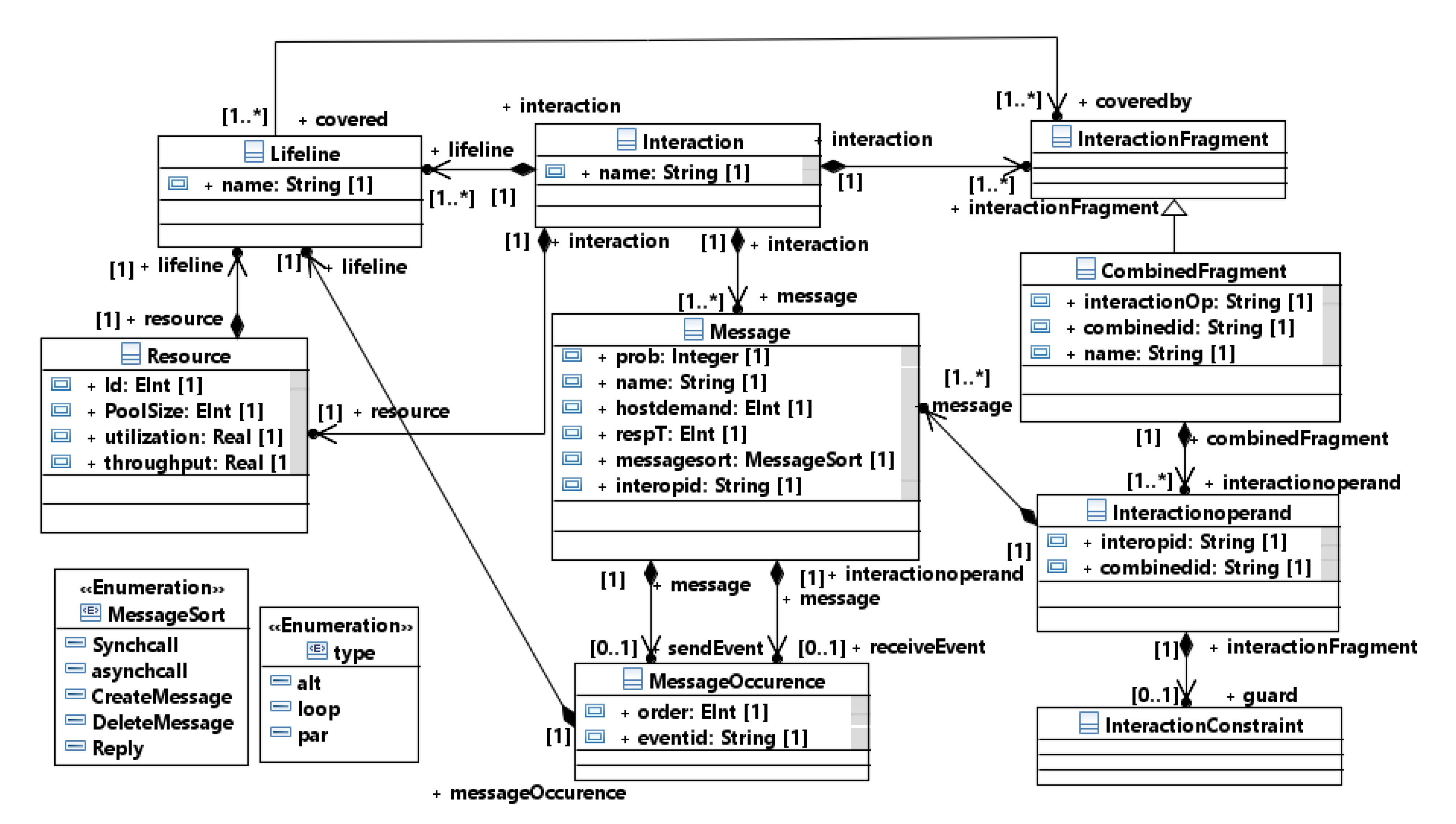
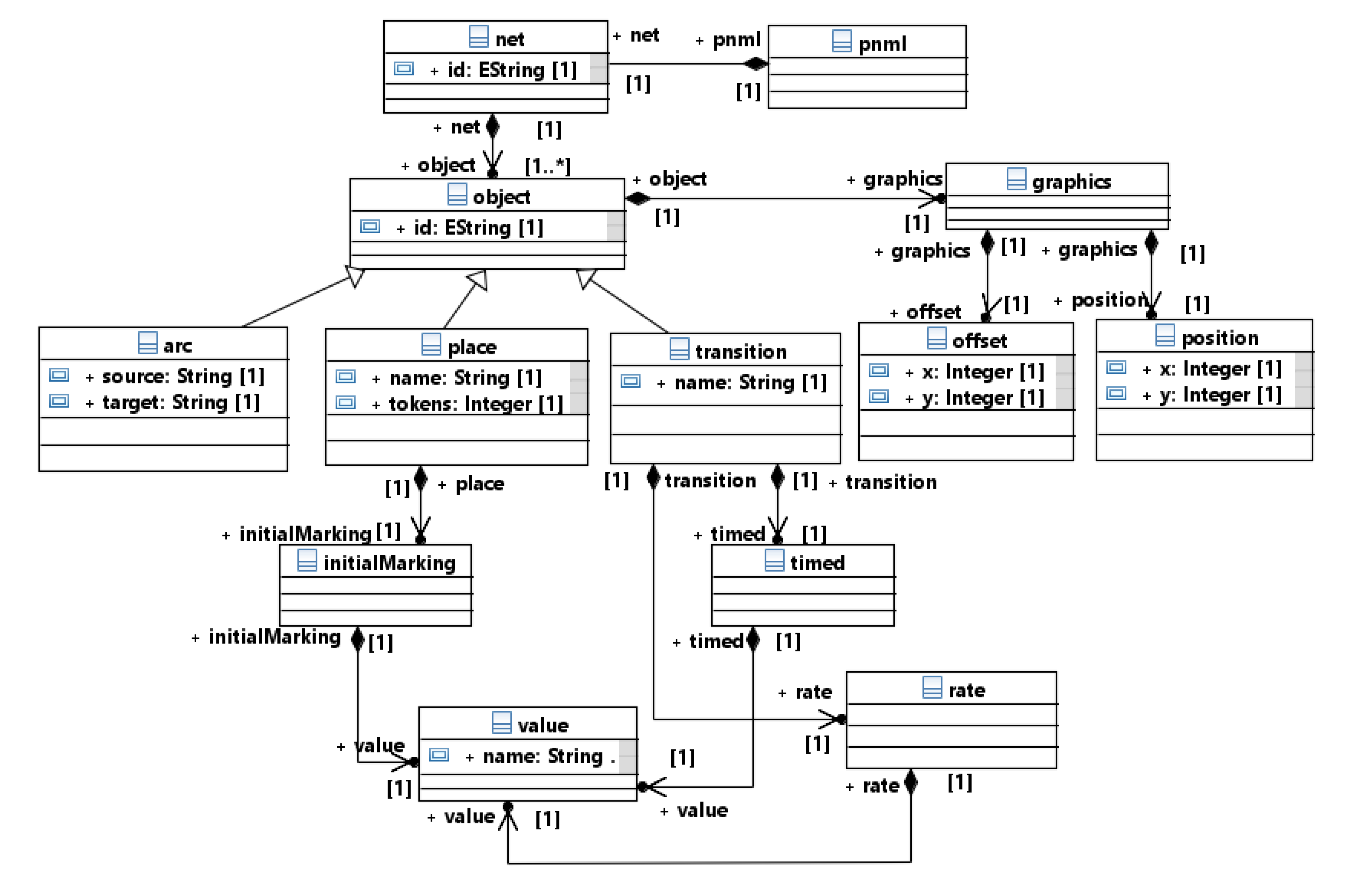
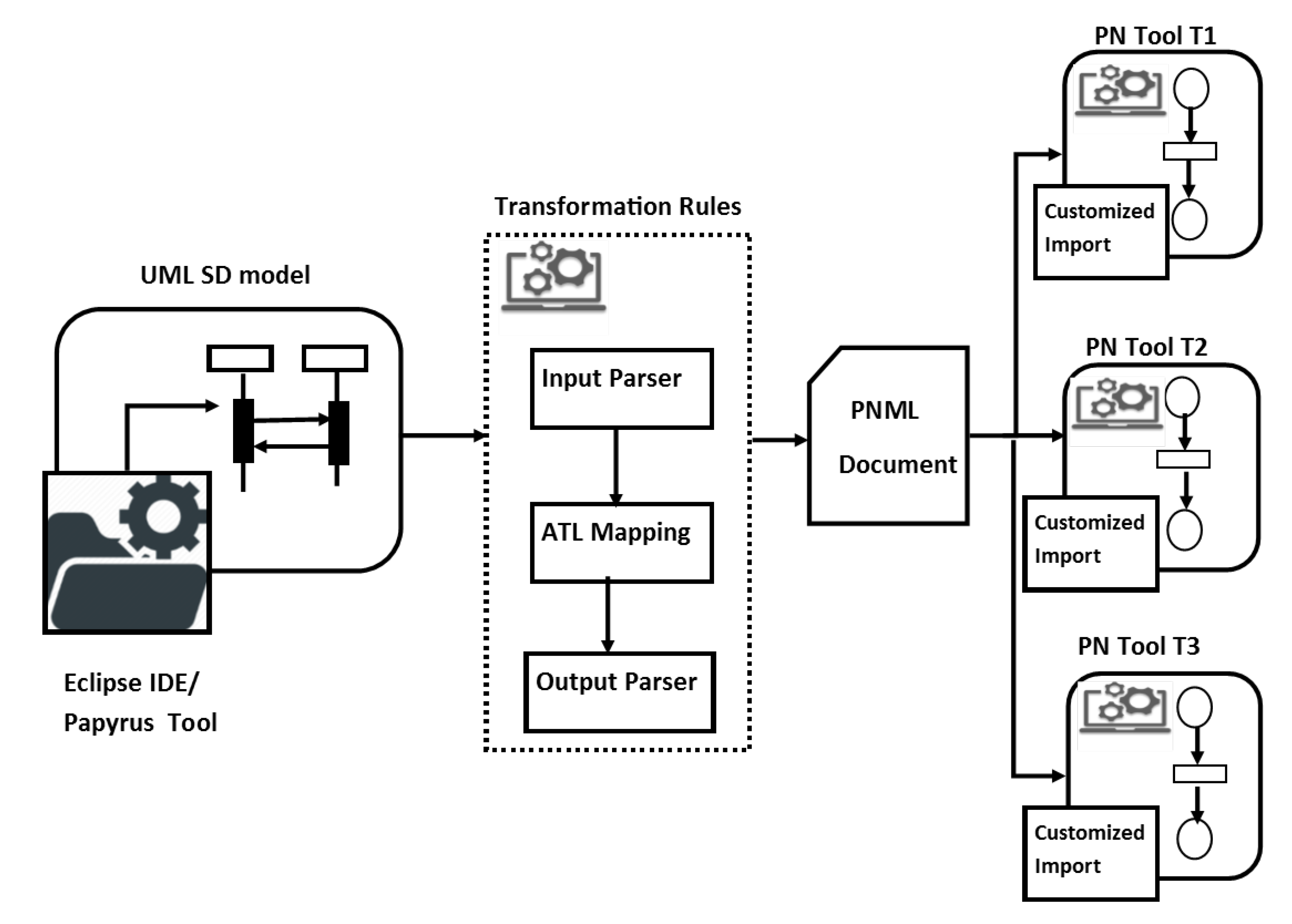
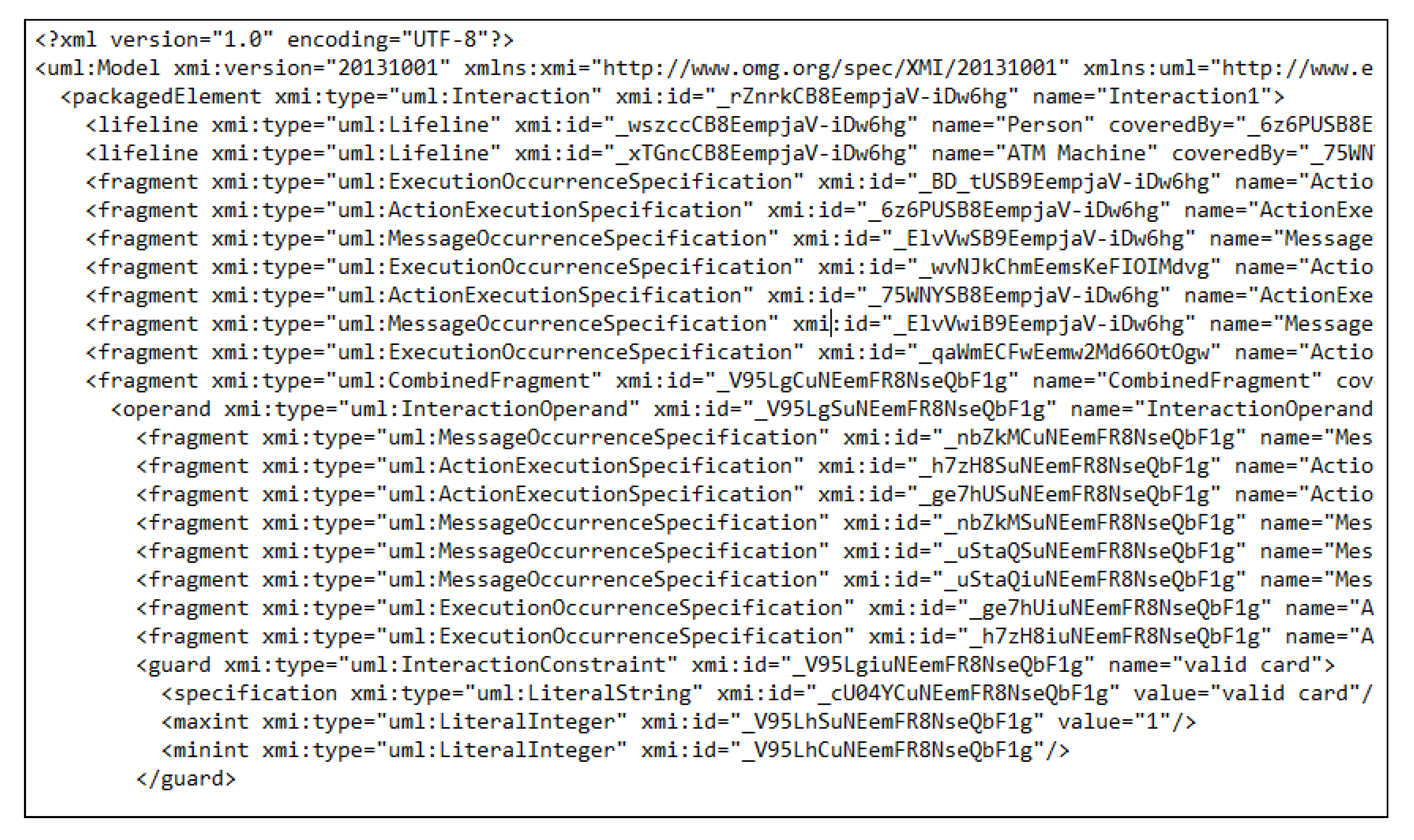
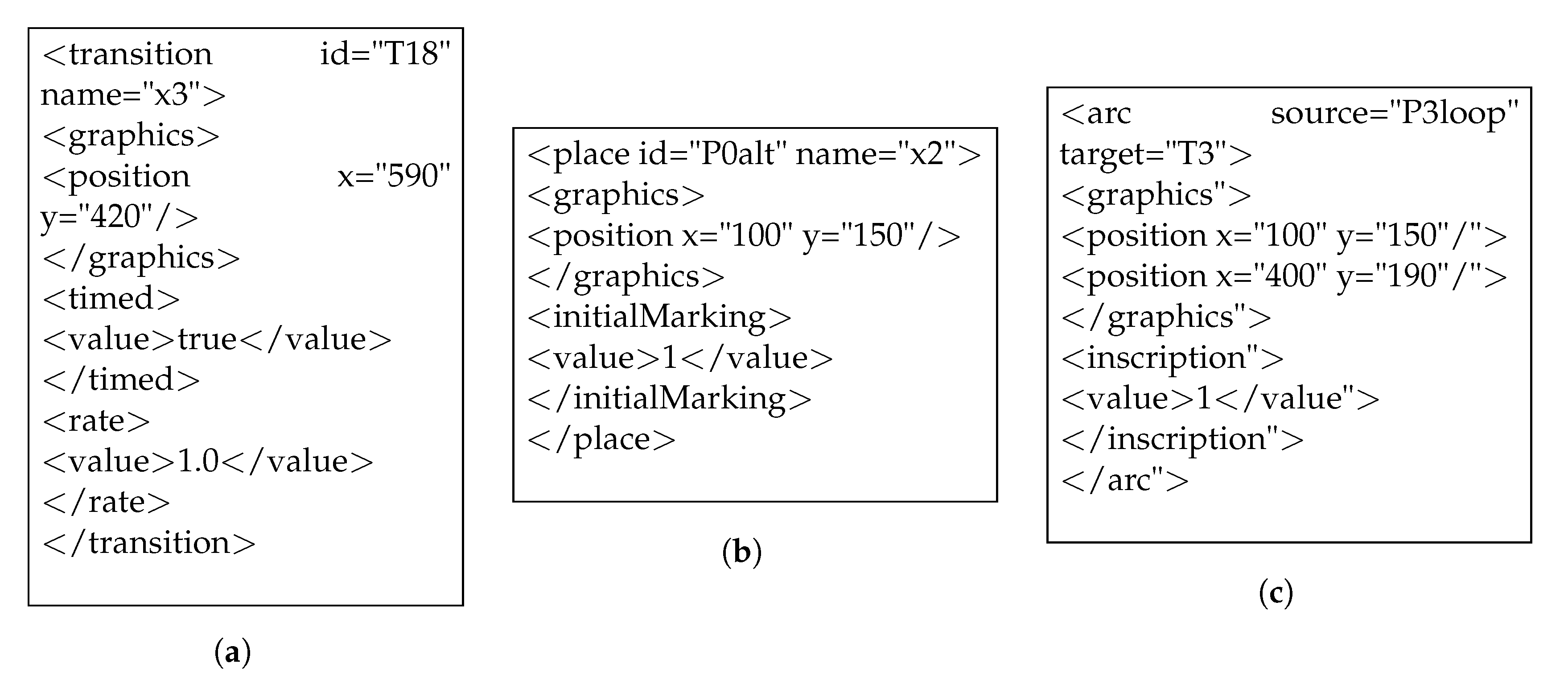
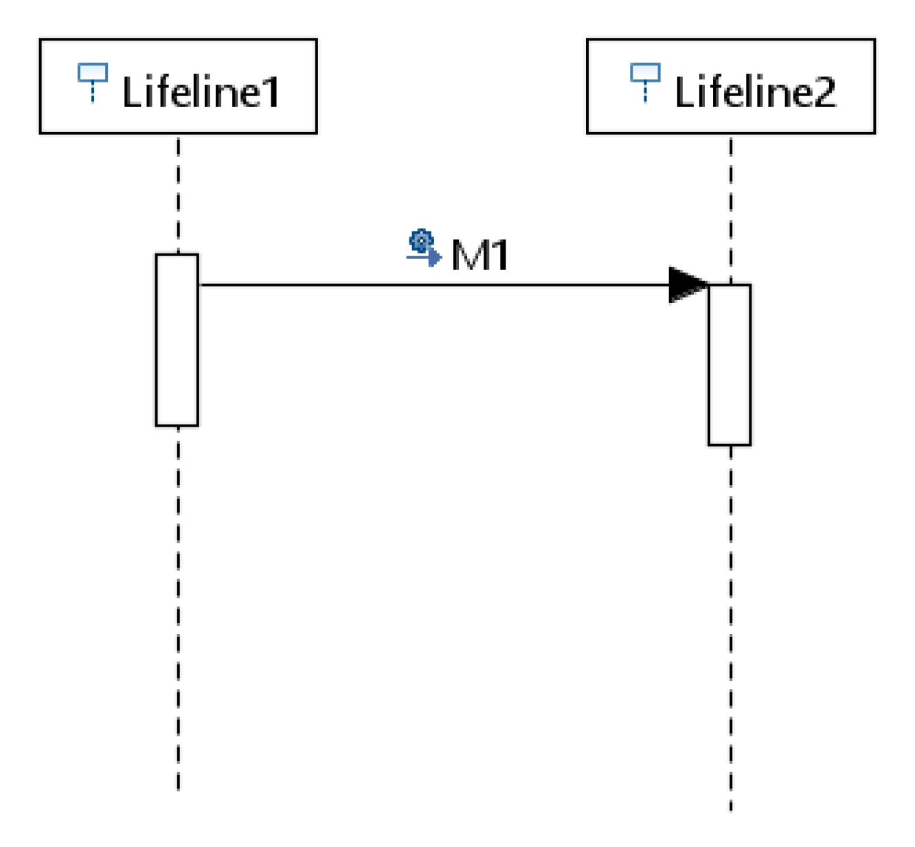
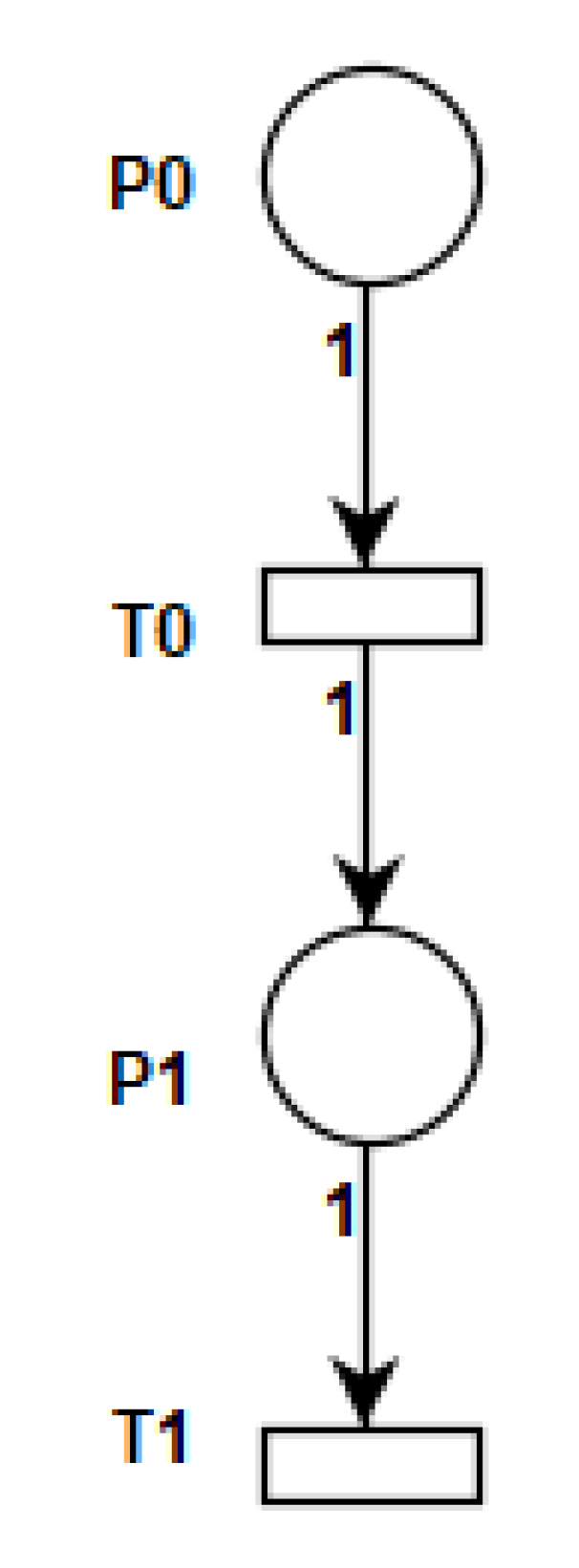
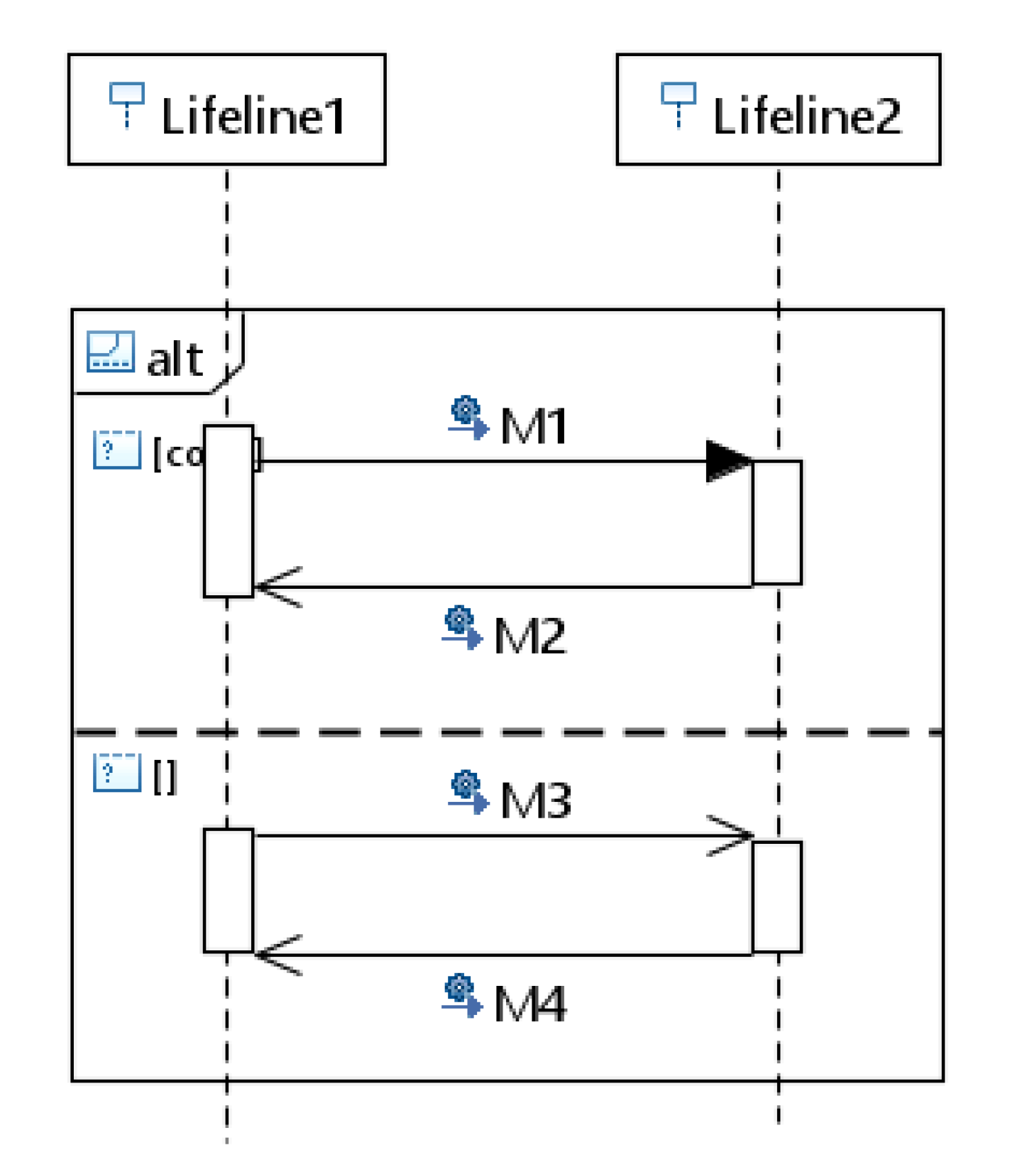
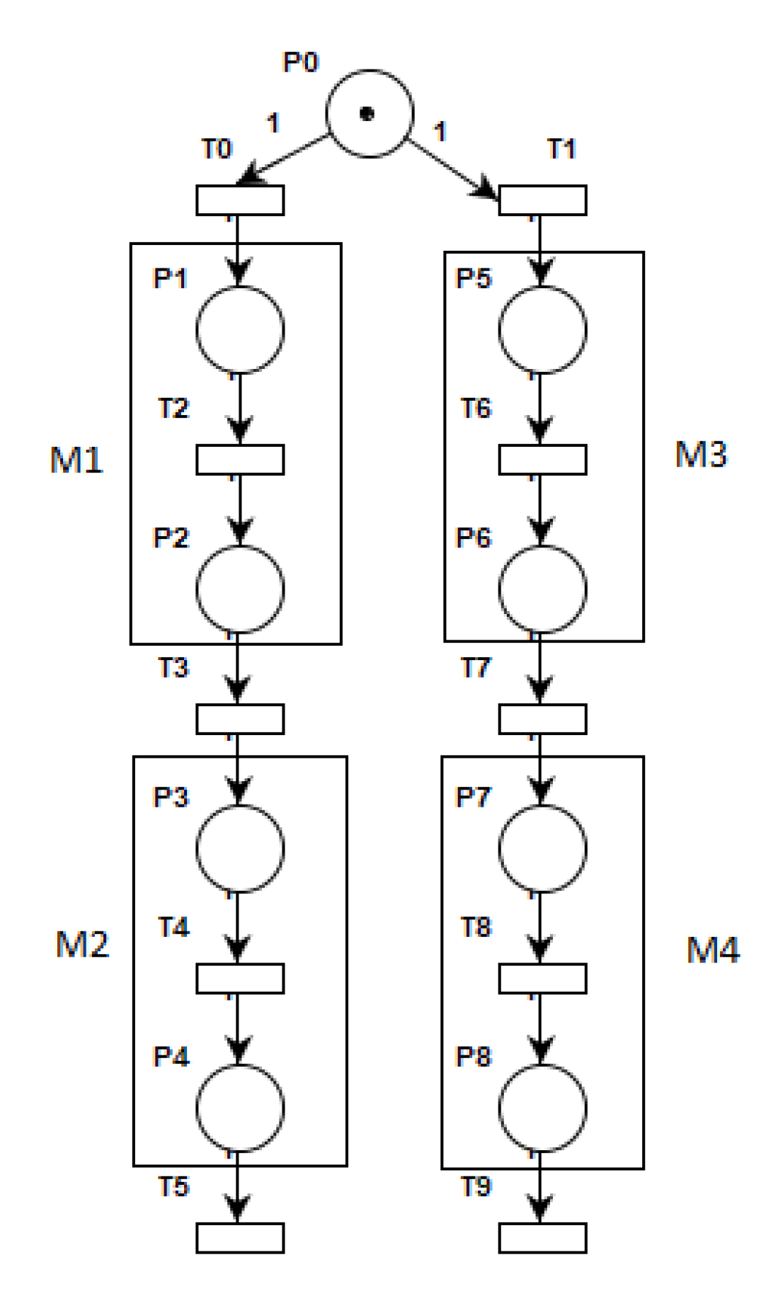
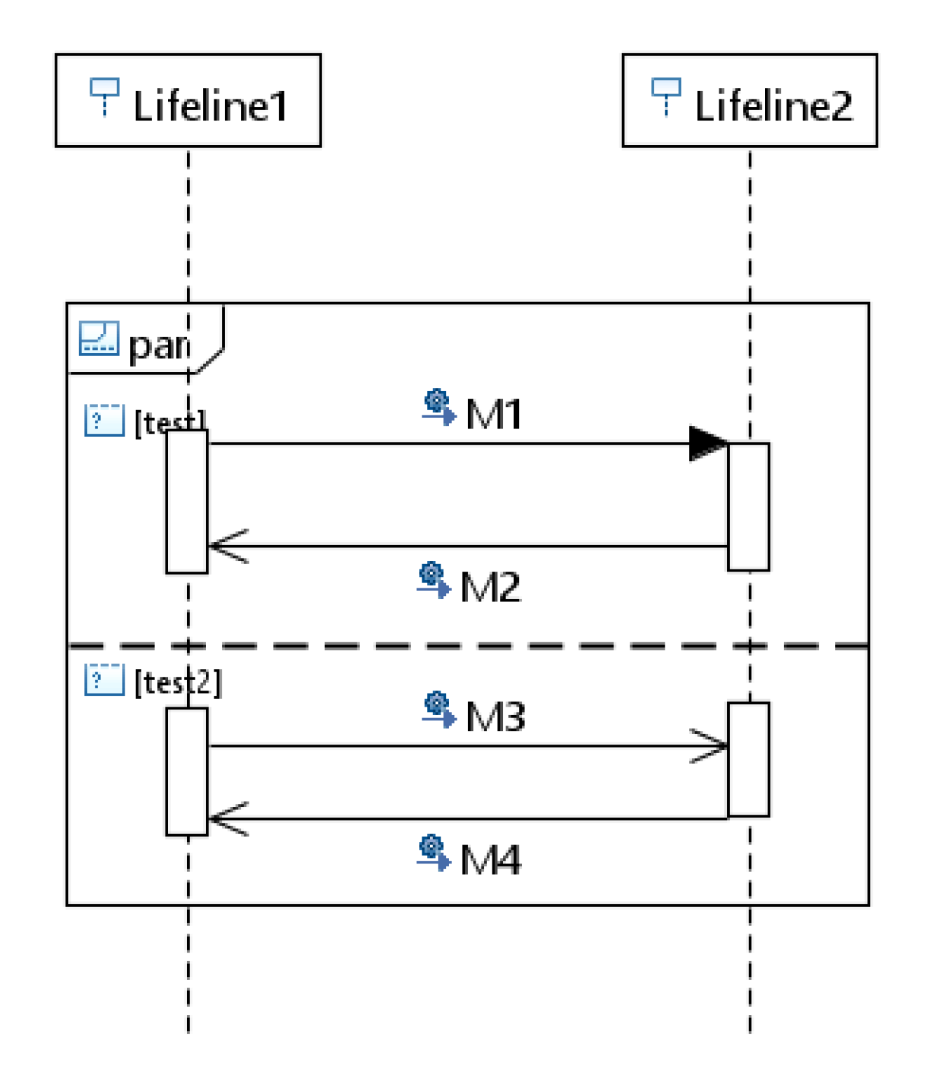
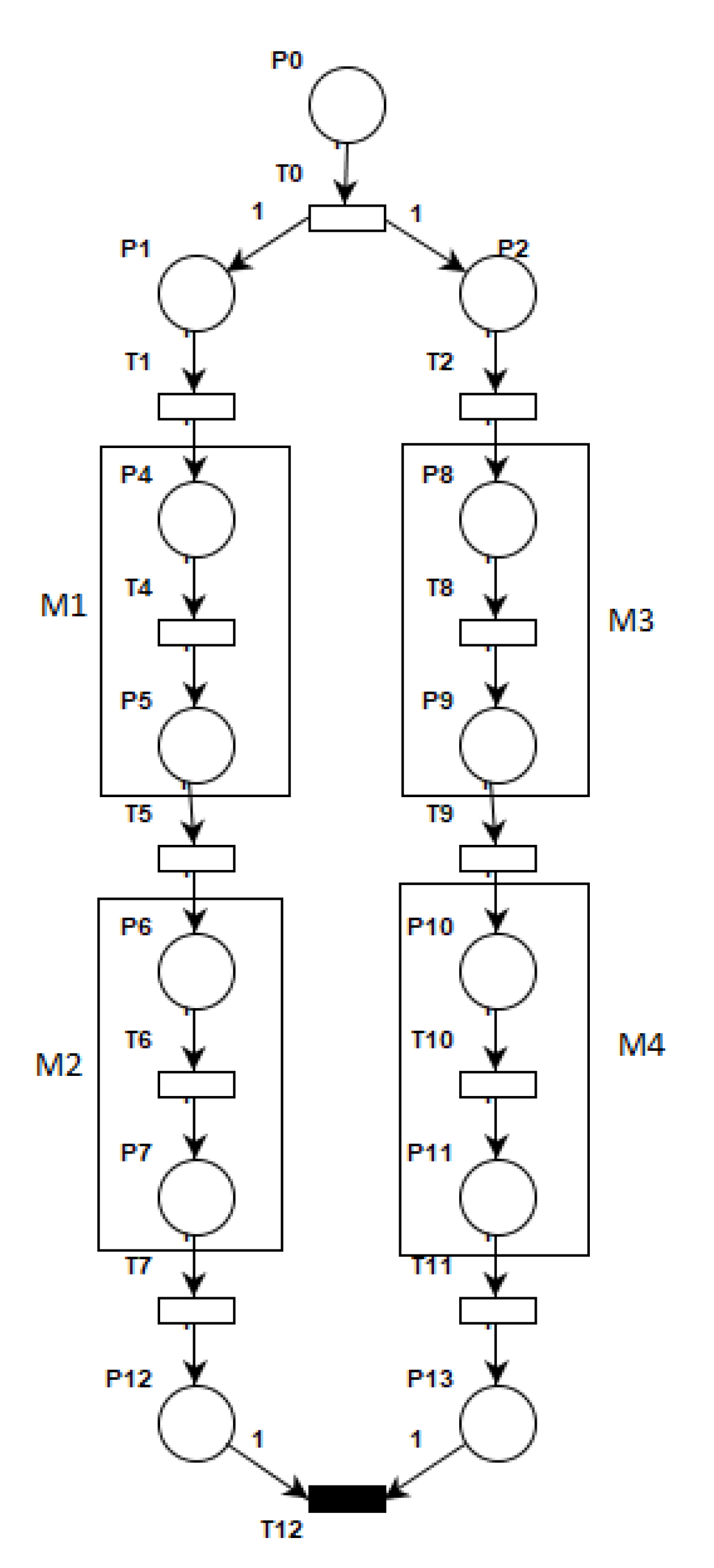
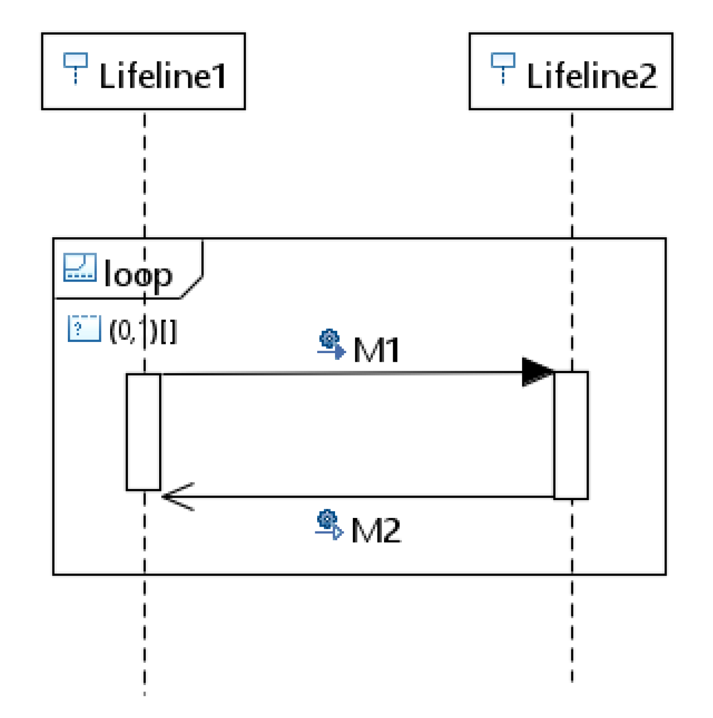
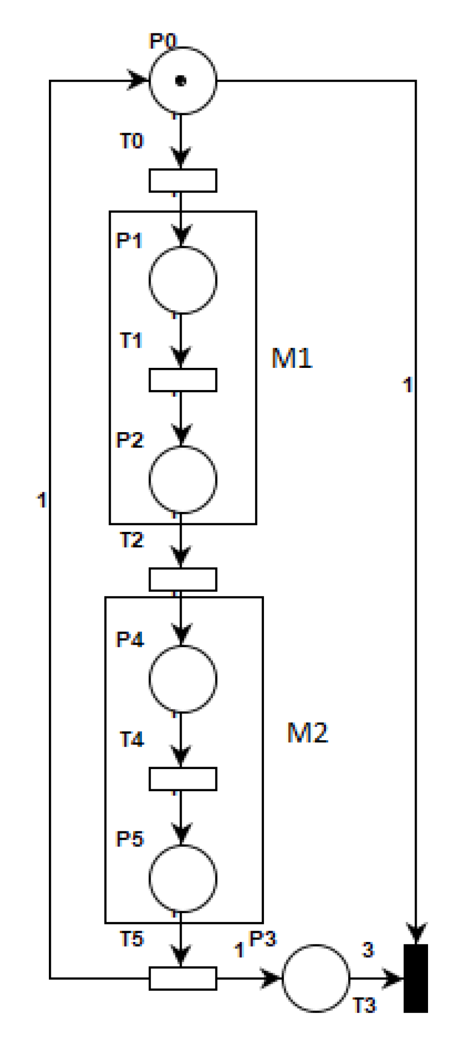
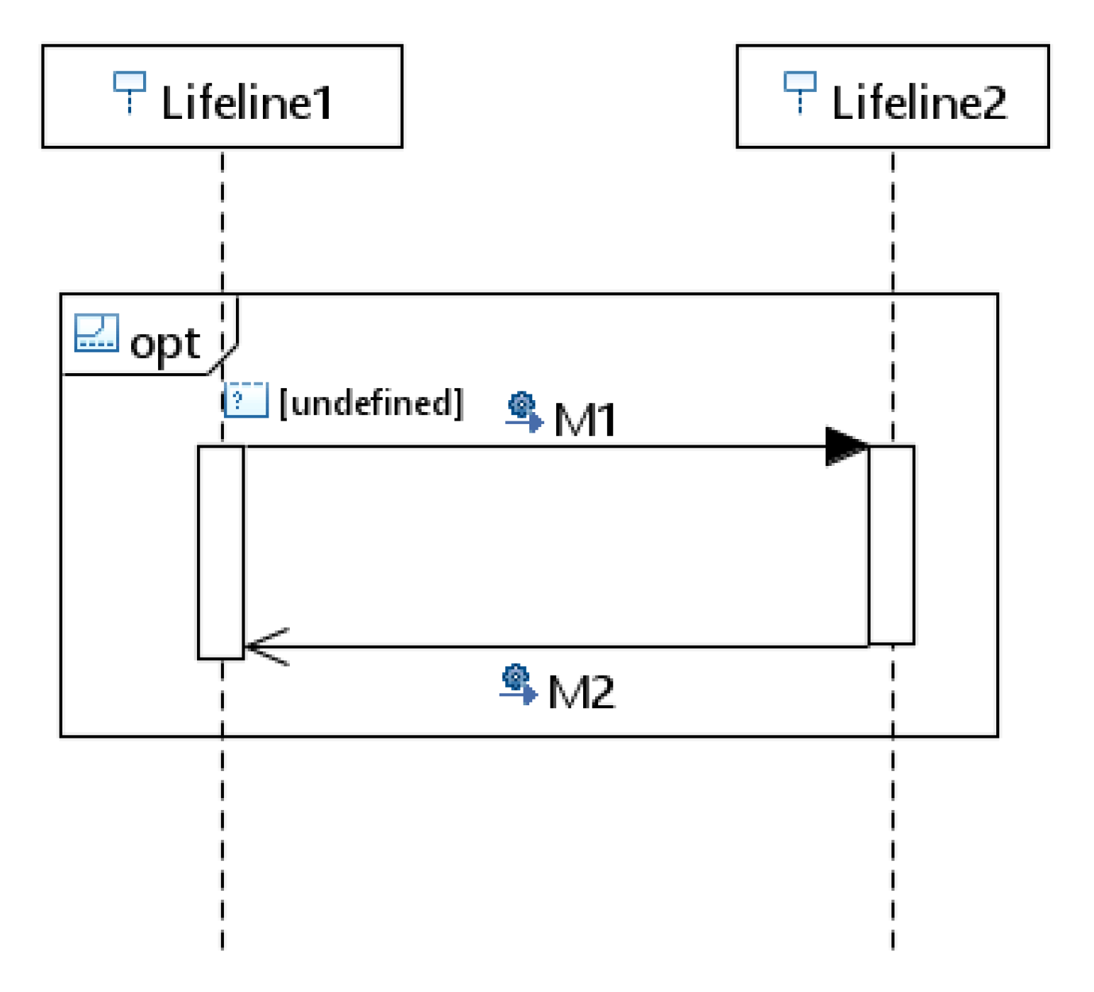
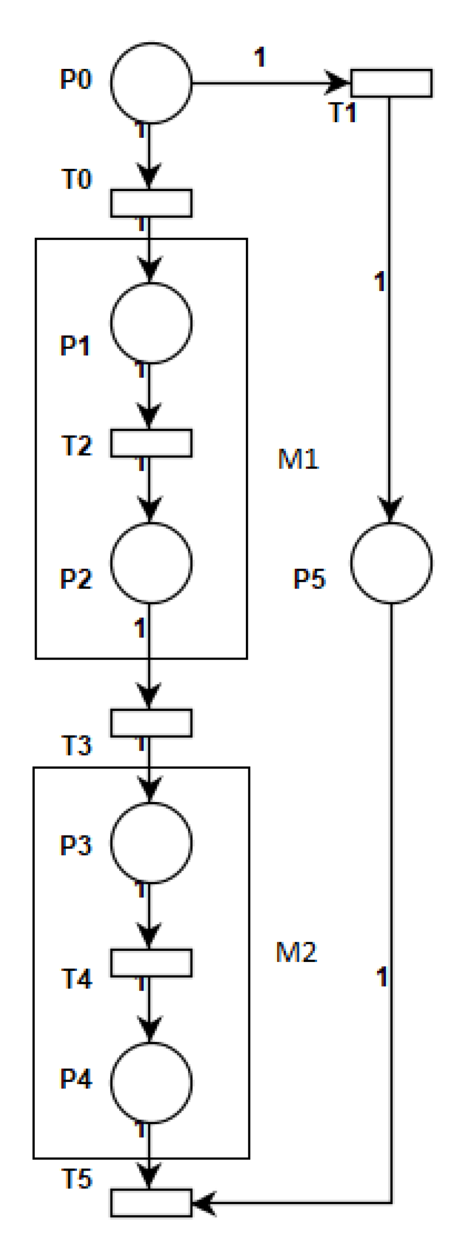
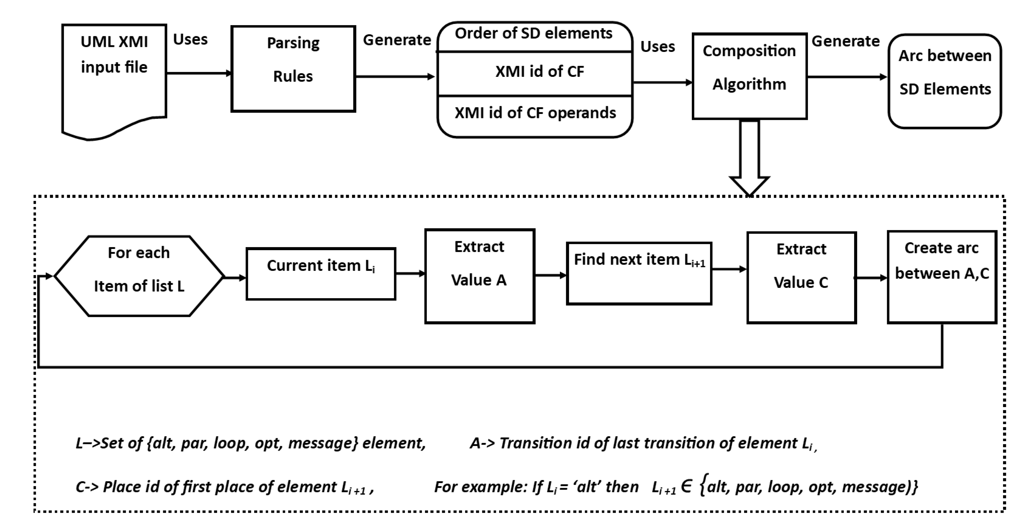
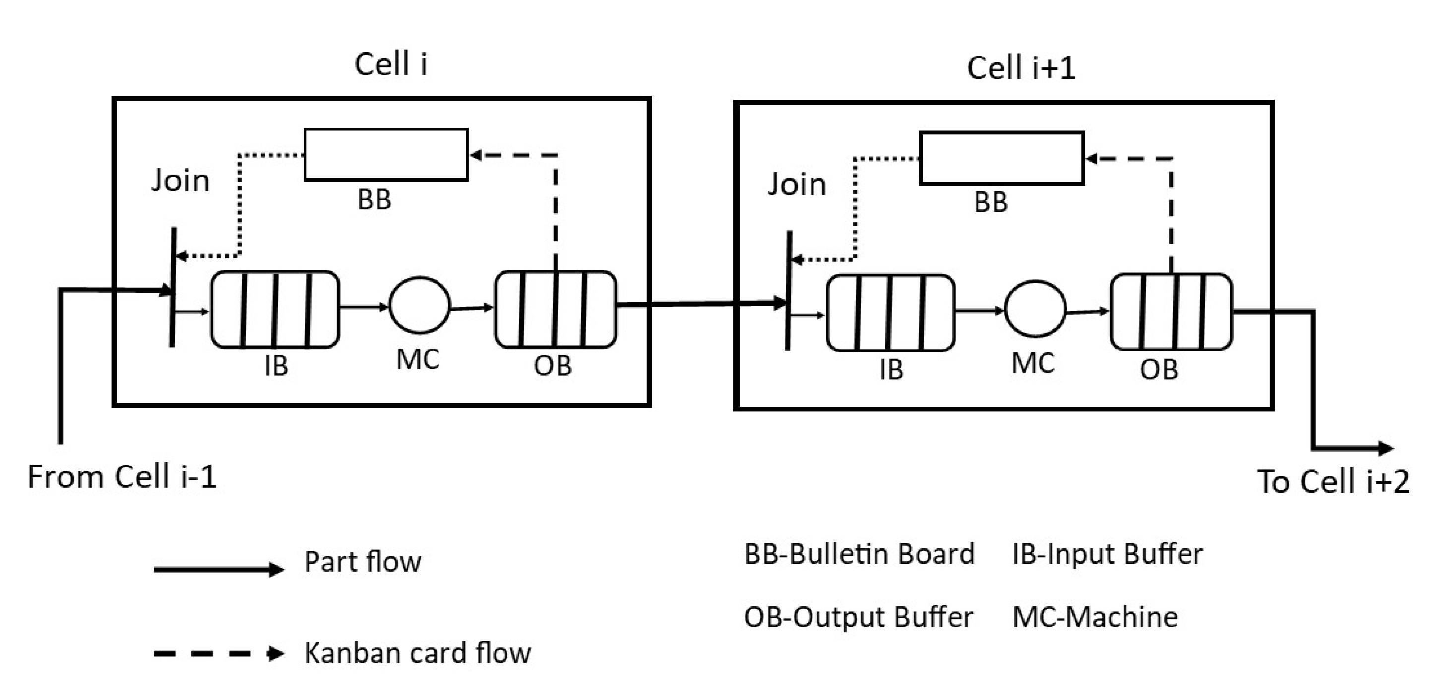
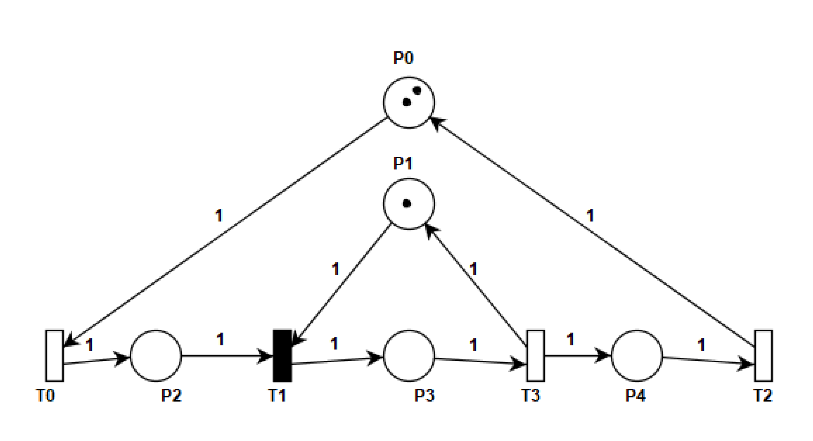
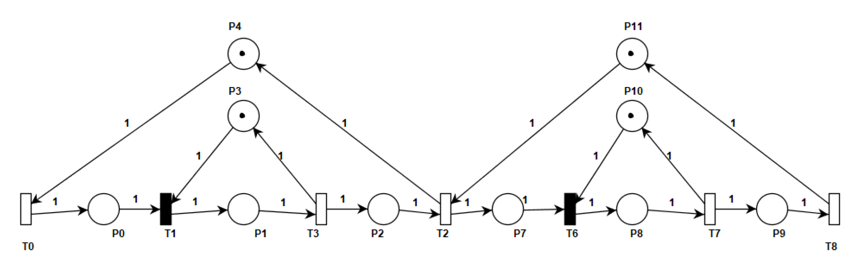
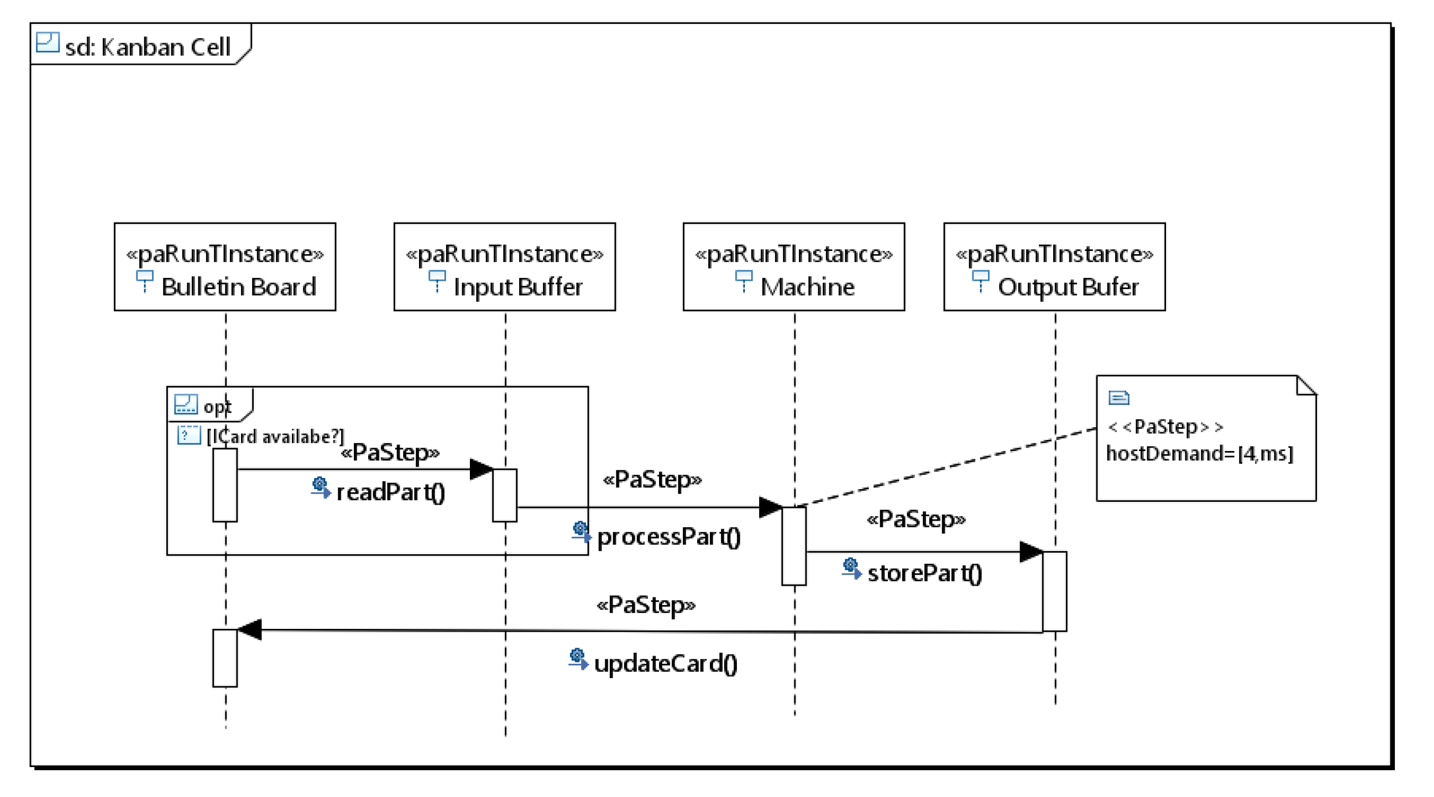
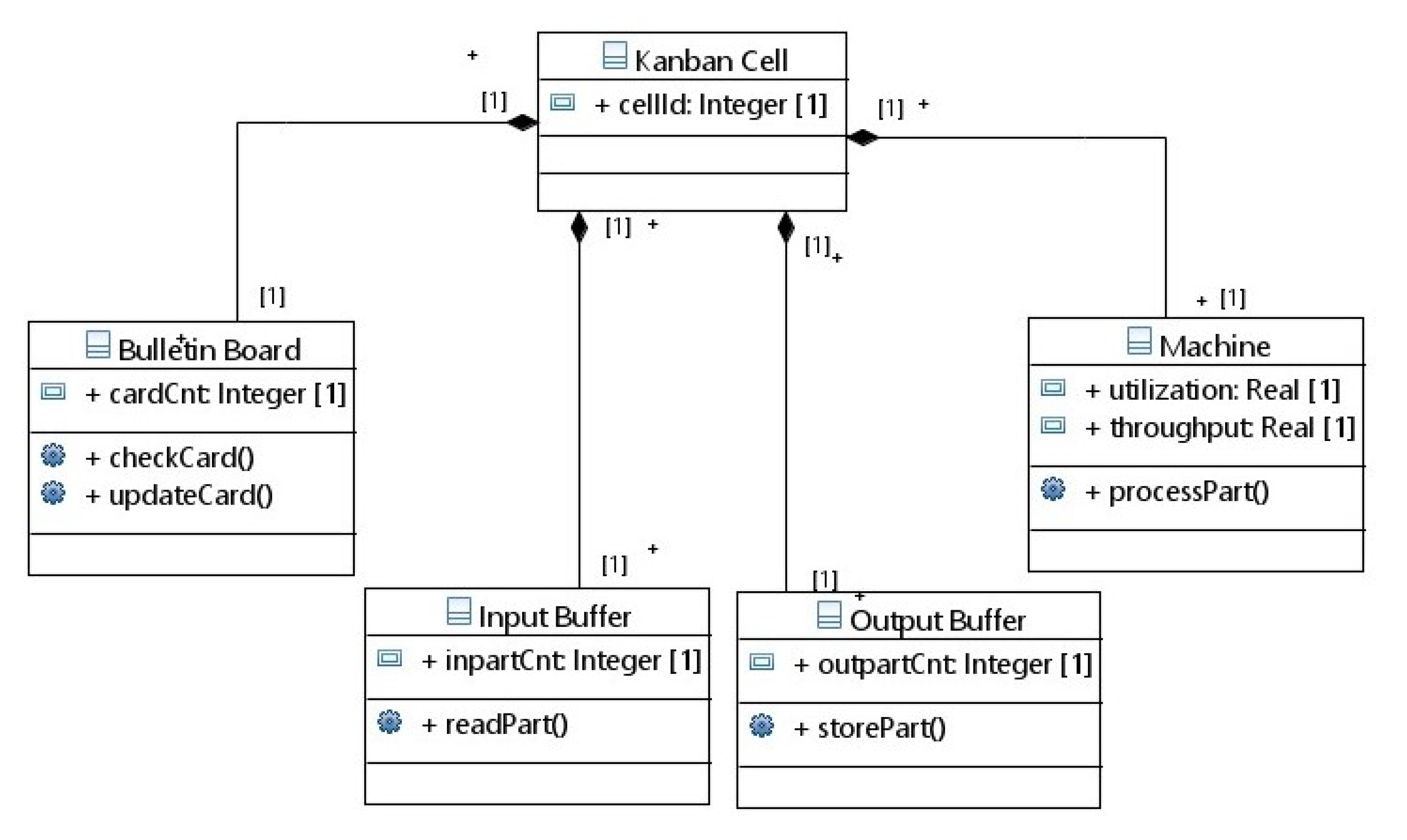
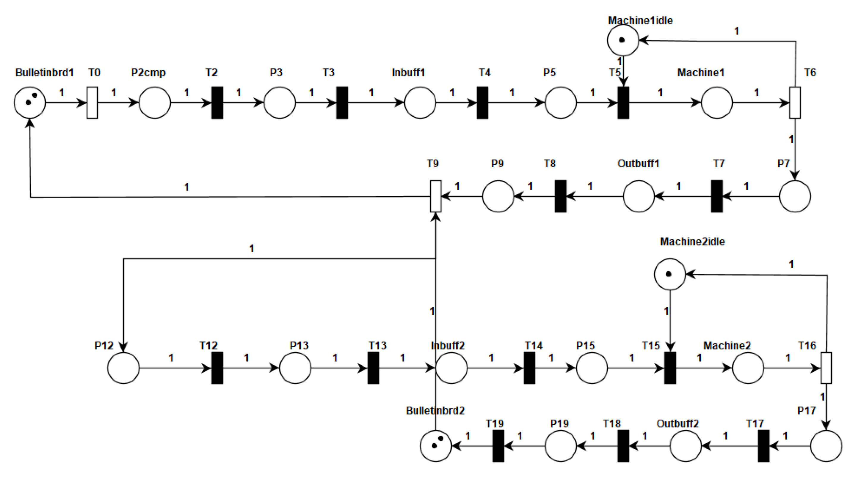
Table 1.
Mapping of MARTE PAM profile concepts.
| Concepts | MARTE STereotypes | MARTE Sub-Profile |
|---|---|---|
| Workload Event | <<PaRunTInstance>> | GQAM_Workload |
| Run Time Instance | <<PaRunTInstance>> | UML::Classes::Kernal |
| Logical Resource | <<PaLogicalResource>> | MARTE::GRM |
| Units of scenario | <<PaStep>> | MARTE::GQAM |
| Communication step | <<PaCommStep>> | MARTE::GQAM |
| Execution Host | <<GaExecHost>> | MARTE::GRM |
Table 2.
Description of one cell GSPN model.
| Element | Description |
|---|---|
| Represent the bulletin board with tokens within it represents the number of the cards in the cell | |
| A token here represents the condition ’cell C is idle | |
| Represent the input buffer | |
| A token here represents the condition ’cell C is busy | |
| Represent the output buffer | |
| A part and card entering input buffer: Rate assumed (1.0) | |
| A machine starts the processing: Immediate transition no delay | |
| A part entering the input buffer of next cell: Rate assumed (1.0) | |
| Processing of parts by the machine: Rate assumed (4.0) |
Table 3.
Variation in the System Throughput.
| Number of Cards | Throughput of the Kanban Petri Net | Throughput of the Derived Petri Net |
|---|---|---|
| 1 | 0.36 | 0.36 |
| 2 | 0.54 | 0.54 |
| 3 | 0.65 | 0.65 |
| 4 | 0.72 | 0.72 |
| 5 | 0.76 | 0.76 |
| 6 | 0.79 | 0.79 |
| 7 | 0.82 | 0.82 |
| 8 | 0.84 | 0.84 |
| 9 | 0.85 | 0.85 |
| 10 | 0.87 | 0.87 |
Table 4.
Part of rechability set of the derived Petri net.
| Marking | P3 | P10 |
|---|---|---|
| M0 | 1 | 1 |
| M1 | 0 | 1 |
| M2 | 1 | 1 |
| M3 | 1 | 0 |
| M4 | 1 | 1 |
| M5 | 0 | 0 |
| M6 | 0 | 1 |
| M7 | 1 | 0 |
| M8 | 1 | 1 |
Table 5.
Variation in the resource utilization.
| Number of Cards | Utilization of Place P3 | Utilization of Place Machine1idle |
|---|---|---|
| 1 | 10% | 10% |
| 2 | 14% | 14% |
| 3 | 17% | 17% |
| 4 | 19% | 19% |
| 5 | 20% | 20% |
| 6 | 20% | 20% |
| 7 | 21% | 21% |
| 8 | 22% | 22% |
| 9 | 22% | 22% |
| 10 | 22% | 22% |
Publisher’s Note: MDPI stays neutral with regard to jurisdictional claims in published maps and institutional affiliations. |
© 2020 by the authors. Licensee MDPI, Basel, Switzerland. This article is an open access article distributed under the terms and conditions of the Creative Commons Attribution (CC BY) license (http://creativecommons.org/licenses/by/4.0/).
Share and Cite
MDPI and ACS Style
Shailesh, T.; Nayak, A.; Prasad, D. An UML Based Performance Evaluation of Real-Time Systems Using Timed Petri Net. Computers 2020, 9, 94. https://0-doi-org.brum.beds.ac.uk/10.3390/computers9040094
AMA Style
Shailesh T, Nayak A, Prasad D. An UML Based Performance Evaluation of Real-Time Systems Using Timed Petri Net. Computers. 2020; 9(4):94. https://0-doi-org.brum.beds.ac.uk/10.3390/computers9040094
Chicago/Turabian StyleShailesh, Tanuja, Ashalatha Nayak, and Devi Prasad. 2020. "An UML Based Performance Evaluation of Real-Time Systems Using Timed Petri Net" Computers 9, no. 4: 94. https://0-doi-org.brum.beds.ac.uk/10.3390/computers9040094
Note that from the first issue of 2016, this journal uses article numbers instead of page numbers. See further details here.