
Correcting for Random Budgets in Revealed Preference Experiments

Department of Economics, The Ohio State University, Columbus, OH 43210, USA
*
Author to whom correspondence should be addressed.
Games 2022, 13(2), 30; https://doi.org/10.3390/g13020030
Submission received: 18 February 2022
/
Revised: 1 April 2022
/
Accepted: 6 April 2022
/
Published: 11 April 2022
(This article belongs to the Special Issue Developing and Testing Theories of Decision Making)
Abstract
:Experiments on revealed preference often use budget sets that are randomly and independently drawn according to some criteria for each participant. However, this means that the budget sets faced by different individuals are not the same. This paper proposes a method to control for these differences. In particular, we control for the “power” of different budget sets by examining the consistency of an individual’s choices relative to some simulated baseline behavior conditional on budgets faced by the individual. We apply this methodology to two existing experimental datasets. Our results show that failure to account for this variation results in a bias when looking directly at measures of choice consistency and the sign of this bias depends on the measure being used. However, controlling for this variation does not change the correlation between measures of choice consistency and observable demographic characteristics like income and education.
1. Introduction
The revealed preference approach has developed various “measures of choice consistency” to describe how consistent an individual’s choices are with utility maximization. Recently, experiments have made use of revealed preference methods to investigate how choice consistency correlates with certain demographic factors. For example, Choi et al. [1] look at how choice consistency varies with income and wealth. Cettolin et al. [2] investigate the relationship between stress and consistency. Li et al. [3] look at whether medical students have more consistent choices than the general population. In these experiments, the method used to select budgets faced by subjects often uses random budgets that differ for each individual. For example, Choi et al. [4] use a method to randomly select budgets that satisfy certain criteria where the budgets are allowed to differ between subjects. This method takes the selection of budgets outside of the hands of the researcher, but makes it difficult to compare across subjects since the budget sets almost always differ between subjects. We call this procedure the random budgets method.
In this paper, we take a closer look at the random budgets method and its interaction with various measures of choice consistency. The ability of a collection of budget sets to detect violations of utility maximization is often refered to as the “power” of the test of rationality following the language of Bronars [5]. One caveat with the random budgets method is that individuals have different budgets and this leads to ex-ante differences in the power of the test. As such, it becomes difficult to assess whether one individual is more “rational” (meaning their choices are more consistent with utility maximization) than another since this difference may be attributed to the different budgets. Naturally, it becomes necessary to account for this variation when comparing measures of choice consistency across subjects.
A common method to account for different budget sets having different abilities to detect choice consistency is to use methods from Bronars [5]. Bronars [5] proposes to compare whether an individual’s choices are “more rational” than random choices made from the budgets. Experiments using the random budget method currently use a variation of the procedure from [5]. We call the existing method a random budgets benchmark. This benchmark compares a subject’s choice consistency to a large distribution of simulated individuals who choose randomly and uniformly over random budgets selected using the same criteria as the experiment (examples include Choi et al. [1], Cettolin et al. [2], Li et al. [3], Choi et al. [6]). This means that the budgets for the simulated individuals are different from the ones observed by the subjects. Thus, from the logic above, the simulations are not directly comparable to the subjects. We propose a different way to account for the variation of budget sets using the individual budgets benchmark. Under this benchmark, we perform the Bronars comparison for each subject by simulating individuals who choose randomly and uniformly over the same budgets faced by the subject. This method corrects for the budgets an individual faces and we can compare individual behavior relative to their individual level benchmarks. For example, we can compare relative percentile ranks for different measures of choice consistency across subjects.
As an application, we compare the random budgets benchmark to the individual budgets benchmark using the datasets of Choi et al. [6] and Choi et al. [1]. Both datasets were generated by an experiment to elicit risk preferences. For the purposes of this paper, we focus on two measures of choice consistency: the critical cost efficiency index (CCEI) [7] and the Houtman-Maks index (HMI) [8]. The CCEI looks at the degree to which budgets need to be perturbed for choices to be consistent with utility maximization. The HMI looks at the maximal subset of the budgets that is consistent with utility maximization.
We find that the random budgets benchmark leads to bias relative to the individual budgets benchmark. Furthermore, the sign of the bias is sensitive to the measure of choice consistency. For the Choi et al. [6] dataset, we observe that average CCEIs under the random budgets benchmark is lower compared to those simulated under our individual budgets benchmark. This implies that there is an upward bias when comparing the CCEIs under the random budgets benchmark. Thus, not accounting for the individual’s budgets suggests that individuals are more consistent than they are for their budgets. For HMI, we find the opposite result. Here, the average random budgets benchmark for HMI is higher than average individual budgets benchmark. Thus, using the random budgets benchmark suggests that individuals are less rational than they are relative to the budgets they faced in the experiment. Qualitatively, we observe similar results for the Choi et al. [1] dataset when looking at the HMI. In contrast, for the Choi et al. [1] dataset the random budgets benchmark of CCEI is almost centered around the average individual benchmarks which leads to no obvious bias.
We also examine how these methods might affect correlation between choice consistency and socio-economic indicators. One concern is that the correlation between choice consistency and observable characteristics may be driven by noise when using the random budget method. The reason for this concern is that correlations might result from the omitted variable of how likely the random budget sets can detect choice consistency. Theoretically, these results should be independent of individual co-variates, but when a study has a small sample of individuals or a small number of budget sets this could occur. We investigate whether controlling for the benchmark ability of budgets to detect choice consistency affects the correlations between individual choice consistency and observed demographic characteristics. Using data from Choi et al. [1] with 1182 individuals and 25 budget sets, we find that the average individual budget benchmark CCEI (HMI) is positively correlated with an individual’s CCEI (HMI). However, controlling for the average individual budget benchmark has no affect on correlations between demographic characteristics and measures of choice consistency. Our results provide evidence suggesting that the random budget method can be used to examine correlations between individual choice consistency and observable characteristics even when there are only 25 budget sets.
This paper adds to the body of literature that focuses on application and interpretation of revealed preference tests (see Crawford and De Rock [9] for a survey). Recent developments have focused on incorporating the power of revealed preference tests in empirical analysis using a measure of predictive success introduced in Beatty and Crawford [10]. Andreoni et al. [11] expand on the Bronars power index and introduce additional power measures that use observed choices to generate the data generating process for the simulated random choices. Demuynck [12] provides ways to conduct statistical inference with such measures on a population of subjects. Our individual budgets benchmark is similar in flavor to the measure of predictive success from Beatty and Crawford [10] and can be expanded to incorporate power measures outlined in Andreoni et al. [11]. Lastly, there is a notable paper by Costa-Gomes et al. [13] where individuals face the same budget sets, but the budget sets where individuals make a choice can differ between individuals since they are not forced to make every choice. In this case, Costa-Gomes et al. [13] perform a Bronar’s correction based on the budget sets where individuals made choices. This is similar to the individual budgets benchmark.
The rest of the paper is structured as follows. Section 2 presents the model, measures of choice consistency, and the power of revealed preference tests. Section 3 discusses the problem of random budgets and defines the random budget and individual budget benchmarks. Section 4 presents some applications to existing datasets. Section 5 provides our final remarks.
2. Model and Measures of Choice Consistency
We focus on the revealed preference framework for demand from Afriat [7] and Varian [14]. Consider a decision maker (DM) who chooses consumption bundles of goods from a linear budget set with prices . Define the dataset of the DM’s chosen consumption bundle at prices by . We say that the dataset is rationalized by utility maximization when there exists some utility function such that, for all t, if , then . Intuitively, a dataset is rationalized by utility maximization when there exists a utility function where each chosen bundle provides a weakly higher utility than the other feasible bundles. Similar to other work on revealed preference, we assume that the utility function is locally non-satiated (a utility function is locally non-satiated when for every bundle x and for every , there exists a bundle y such that and ).
Definition 1
(Direct Revealed Preference). A bundle is directly revealed preferred to bundle x, written when . A bundle is strictly directly revealed preferred to bundle x, written , when .
Intuitively, when is chosen at prices and x is affordable, i.e., (), then it must be the case that is (strictly) preferred to x. We define (indirect) revealed preference as follows:
Definition 2
(Revealed Preference). A bundle is revealed preferred to x when there is a sequence of observations such that .
The revealed preference relation is the transitive closure of the direct revealed preference relation. Note that being directly revealed preferred is a special case of the revealed preference relation. We define the generalized axiom of revealed preference (GARP) below.
Definition 3
(GARP). Dataset satisfies GARP if for every pair of observations , if is revealed preferred to , then it is not the case that .
GARP essentially rules out all possible violations of transitivity on observed data with respect to the revealed preference relation. Varian [14] shows that consistency with utility maximization is equivalent to a dataset satisfying GARP. The result is recorded below.
Proposition 1
(Varian [14]). Dataset can be rationalized by a locally non-satiated utility function if and only if satisfies GARP.
2.1. Measures of Choice Consistency
While Varian’s result is useful, it does not allow us to distinguish which datasets are “farther away” from utility maximization. This is important because empirical evidence suggests that choices exhibit violations of GARP. To address this problem, many “measures” of choice consistency have been developed to capture the severity of GARP violations observed in the data. We focus on two measures that are most often used: Afriat’s critical cost efficiency index (CCEI) [7], and Houtman-Maks index (HMI) [8]. Other inconsistency measures used in applied work are the inconsistency index from Varian [15], the money pump index from Echenique et al. [16], and the minimum cost index from Dean and Martin [17]. We discuss the CCEI and HMI in detail. We follow the integer programming approach from Demuynck and Rehbeck [18] to construct and compute these measures.
2.1.1. CCEI
The CCEI measures the amount that each budget has to be adjusted to ensure that the dataset is consistent with GARP. Formally, let . We define the relaxed revealed preference relations below.
Definition 4
(Relaxed Revealed Preference). A bundle is relaxed directly revealed preferred to x, written , when . A bundle is relaxed strictly directly revealed preferred to x, written , when . The relaxed revealed preference relation is the transitive closure of .
The CCEI is calculated as follows:
Intuitively, the higher the value for e, the lower the adjustment of budgets needed for the data to satisfy GARP. When the CCEI is one, the dataset either satisfies GARP so it is rationalizable by some locally non-satiated utility function or the violation can be made arbitrarily small (see Murphy and Banerjee [19] for a discussion on an arbitrarily small deviation when the CCEI is one).
2.1.2. HMI
The HMI calculates the maximal subset of the data that is consistent with GARP. Formally, denote to be a subset of observations within the data. The HMI can be calculated as follows:
where is an indicator function that is one when is included in the subset B that rationalizes the dataset and is zero otherwise. The HMI is a measure of how consistent a dataset is with GARP since individuals who have more choices consistent with GARP will have a larger HMI. An HMI of T indicates that the entire dataset satisfies GARP and can be rationalized by a locally non-satiated utility function.
2.1.3. Power of Revealed Preference Tests
One major issue with revealed preference work is that it is difficult to know whether the test has “power” to detect violations. In particular, the structure of the budget sets determines (to some extent) whether violations of GARP can occur and the size of the violation. The experimental literature has focused on using variations of the Bronars measure to calculate the power of a revealed preference test [5]. The idea behind the Bronars measure is to compare the number of GARP violations under the assumption that bundles are chosen randomly from the observed budget sets (see Andreoni et al. [11] for a discussion on different power measures and different computational methods of calculating the Bronars measure).
3. Random Budget Method and Obstacles
Many revealed preference experiments randomly generate budgets for subjects where budgets often differ for each subject (see, for example Choi et al. [1], Cettolin et al. [2], Li et al. [3], Choi et al. [6]). Under this design, each subject faces a sequence of budget sets that have been randomly and independently chosen from a collection of linear budget sets that satisfy certain properties. For the two good case that much of the literature focuses on, the budgets are drawn randomly from the class of budget sets that cross the horizontal-axis between some interval and cross the vertical-axis between some interval . This methodology has been used to investigate choice under uncertainty [1,6], to investigate social preferences [3,20] and to analyze the effect of stress on rationality [2].
The random budgets method makes it difficult to compare choice consistency across individual participants since it is unlikely for two individuals to make decisions over identical budget sets. However, the power to detect violations of GARP is driven by the structure of the budget sets. Since budgets sets are different for each participant, there is a large degree of variation in the power to detect GARP violations. Thus, it is difficult to say whether one individual is more “rational” than another. For example, the difference in rationality may be driven by the fact that the budget sets of the “more rational” individual have lower power to detect violations of GARP.
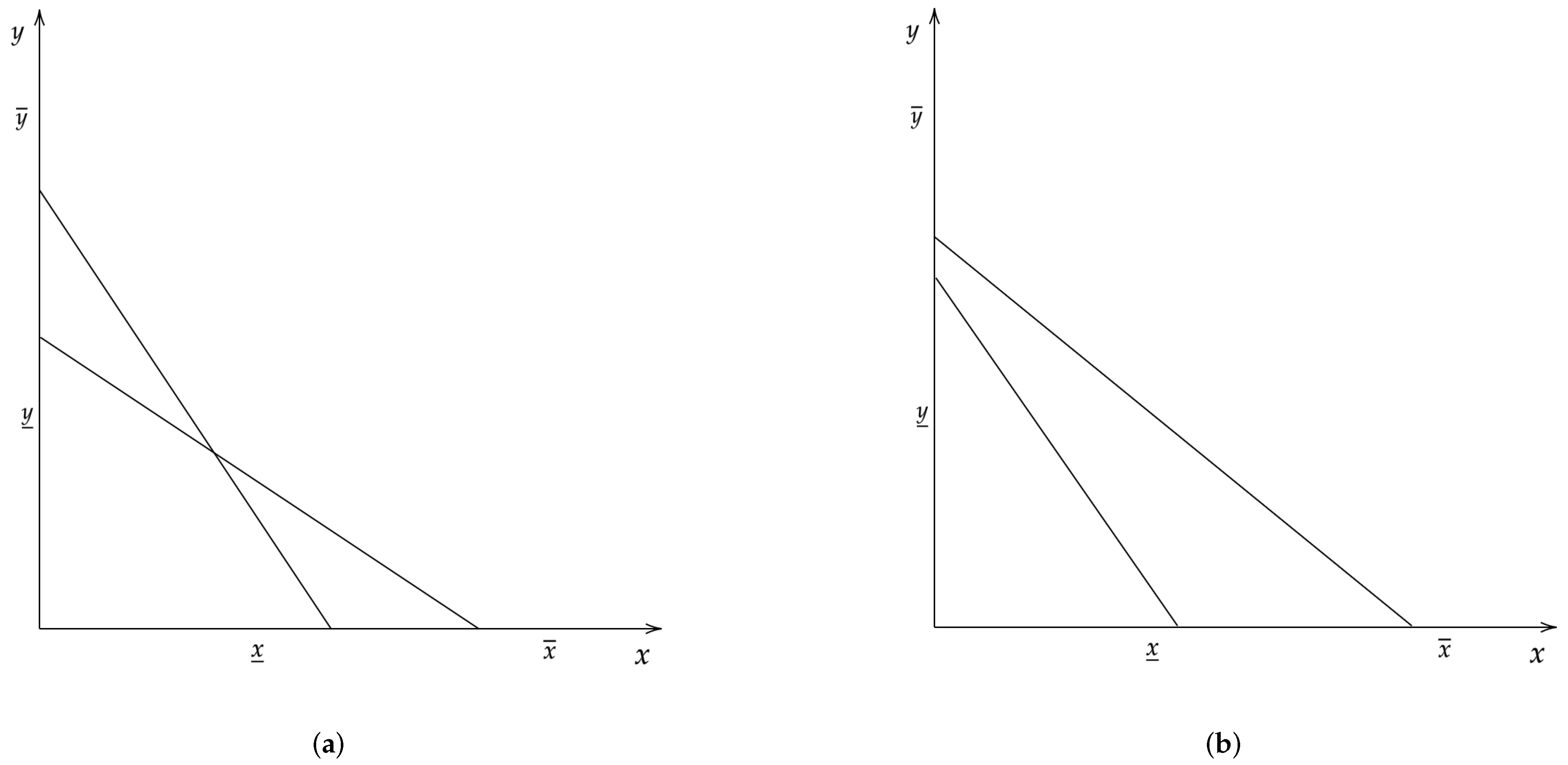
To illustrate an extreme case of this issue, consider the following example of a two good, two budget decision problem in which budgets are drawn randomly as explained above. Figure 1 shows two such budget sets.
A subject facing the budget sets in Figure 1a has an opportunity to violate GARP since the budget sets cross. On the other hand, a subject facing the budget sets in Figure 1b is never going to violate GARP. Thus, ex-ante we expect subjects facing budgets in Figure 1a to have more GARP violations than subjects who choose from budgets in Figure 1b. This means that it would be incorrect to conclude that a subject facing budgets in Figure 1a is less rational than a subject who chose from budgets in Figure 1b since by chance the latter budget can never produce a violation of GARP. We note that as individuals face a larger number of random budgets, such an extreme case as seen in Figure 1 is unlikely to occur.
To account for power, experiments using random budgets such as [6,20] adopt, what we call, the random budgets benchmark. The method proceeds as follows:
- 1.
- Generate a set of random budgets using the same procedure as the experiment;
- 2.
- Simulate uniform choices over each budget;
- 3.
- Compute and record the measure of choice consistency;
- 4.
- Repeat steps 1–3 to create a distribution with S simulated individuals
- 5.
- Compare each individual’s measure of choice consistency to the simulated distribution from 4.
The key point in this method is that budgets for the simulated individuals are chosen in the same manner as that for the participants. In particular, the budgets are chosen randomly and independently of the budgets in the simulation and the budgets of participants. Thus, each round of the simulation has a different set of budgets and a different power to detect violations of GARP. As such, the simulations are not necessarily comparable to the participants.
Correcting for Random Budgets
The nature of the random budgets method does not allow for a clean comparison of choice consistency across different participants. Some budget sets may have low power to detect violations of GARP compared to others. As such, we need a way to account for this variation across different budget sets when comparing individual choice consistency. The random budgets benchmark is not appropriate since the simulated budgets are not the same as those faced by the participants. We later show this can bias how rational subjects are deemed by the measure of choice consistency after correcting for power of the budget set.
We propose an alternative approach which we call the individual budgets benchmark. Here, we propose to use the budgets faced by each individual to produce a set of simulated subjects to compute a baseline measure of the power to detect GARP violations. The method proceeds as follows:
- 1.
- Generate budgets used by the ith individual;
- 2.
- Simulate uniform choices over each budget;
- 3.
- Compute and record the measure of choice consistency;
- 4.
- Repeat steps 2–3 to create a distribution with S simulated individuals
- 5.
- Compare the ith individual’s measure of choice consistency to the simulated distribution from 4.
- 6.
- Repeat steps 1–5 for each individual
For an example of how to compare measures of choice consistency across individuals, we compute the percentile rank of choice consistency relative to the distribution generated by the individual budgets benchmark. This provides a normalization that corrects for the power of the budget sets faced by each individual and is in comparable units. By conducting the individual budgets benchmark, we effectively determine how rational an individual is relative to the benchmark power of their budget sets. An alternative method to compare across individuals is to use the measure of predictive success () proposed by Beatty and Crawford [10] where r is the individual’s measure of choice consistency and a as the average measure generated by the individual budgets benchmark.
In the next section, we apply this methodology to two existing datasets and compare the results to the random budgets benchmark used in the experimental literature.
4. Applications
We focus on datasets from Choi et al. [6] (henceforth CFGK) and Choi et al. [1] (henceforth CKMS). The experimental procedures for both papers follow those outlined in Choi et al. [4]. Each experiment consists of multiple independent and identical rounds (50 for CFGK and 25 for CKMS) of decision making under uncertainty.
In each round, subjects are shown a two-dimensional graph with a budget line and asked to allocate tokens between two accounts x (represented on the horizontal-axis) and y (represented on the vertical-axis). Subjects choose an allocation by picking a point on the budget line for each round. At the end of the experiment, the computer randomly selects one budget and randomly selects an account to pay the subject. For CKMS and the symmetric treatment of CFGK, each account was equally likely to be selected. For the asymmetric treatments of CFGK, one account had a 1/3 chance of being selected. One interpretation of this decision problem is that of allocating assets between two Arrow securities.
The key feature of this experimental design is that the budgets in each round are drawn randomly from a set of available budgets. For each round, the computer randomly selects a budget set that satisfies two properties:
- 1.
- The budget line crosses one axis at or above 50 tokens and;
- 2.
- The budget line crosses both axes at or below 100 tokens.
This randomization is done independent of the budgets chosen within each round and independent of the budgets chosen for other subjects. As a result, there is a large degree of variation in the choice problems across subjects which creates problems when comparing across individual subjects.
As a first step, we follow CFGK and CKMS, and compare each subject to the random budgets benchmark. We simulate 25,000 individuals who randomly and uniformly choose allocations over budget sets that have been randomly selected following the same criteria outlined above. We compare each individual subject to this distribution of simulated individuals.
However, as mentioned earlier, this method faces a drawback in that the simulated individuals’ budget sets are randomly chosen independent of one another. To account for this, we compare each individual subject to the individual budgets benchmark. For each subject, we simulate 500 individuals who randomly and uniformly choose allocations from the same budget sets that the subject faces.
4.1. Results for CFGK
The experiment was conducted at UC Berkeley’s Experimental Social Science Laboratory. Data was collected on 93 subjects recruited from UC Berkeley’s undergraduate student population and staff.
Figure 2 shows how the two benchmarks fare for the CCEI. Figure 2a shows the histogram of averages of the simulated CCEIs. Specifically, the histogram plots the distribution of the averages of the CCEIs (for each subject) simulated under the individual budgets benchmark. There is considerable variation in the simulated CCEIs, with the averages ranging from 0.58 to 0.72. The vertical line represents the average for the 25,000 simulations conducted under the random budgets benchmark which is approximately 0.605. We find that the random budgets leads to a lower average CCEI compared to the individual budgets. This implies that the budgets faced by individual subjects are on average more permissive than can be captured by the random budgets benchmark. Essentially, a simulated individual requires smaller perturbations in their budgets to satisfy GARP. This indicates that subjects are less rational than the random budget benchmark suggests.
This bias is further captured in Figure 2b which plots the empirical CDFs of each individual subject’s percentile rank under both benchmarks. Specifically, we calculate the percentile rank of each individual subject’s CCEI with respect to the distribution of the CCEIs generated by the 25,000 random simulations under the random budget and with respect to the 500 simulations using the same budget sets as the individual. A percentile of X indicates that the subject’s CCEI is higher than of the simulated population. While around 85% of the subjects fall in the 95+ percentile under both benchmarks, we do observe a discrepancy for the remaining population of subjects. In particular, we find percentile ranks to be lower under the individual budgets benchmark compared to random budgets benchmark, a finding consistent with the fact that the individual budgets benchmark have (on average) a higher CCEI. The two distributions are significantly different as indicated by a Wilcoxon signed-rank matched pairs test having a p-value of 0.0117.
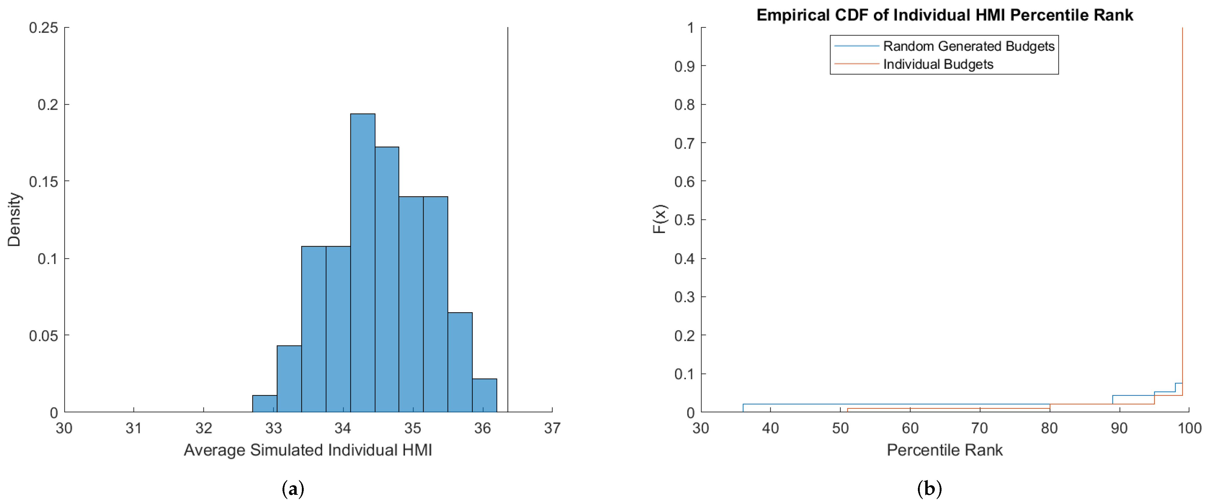
Figure 3 shows the comparison for the two benchmarks for the HMI. Average HMIs under the individual budget benchmarks range from 32.7 to slightly above 36. We observe that the random budgets benchmark results in a higher average HMI (approximately 36.4) compared to the average HMIs generated using the individual budget benchmark. This implies that, on average, the random budget benchmark leads to fewer violations of GARP, compared to the individual budgets benchmark. This indicates that subjects are more rational than suggested by the random budgets benchmark. This is supported in Figure 3b which shows that the CDF of HMI percentile ranks under the individual budgets benchmark first order stochastically dominates the CDF under the random budgets benchmark. Percentile ranks for almost 10% of the subject population are higher under the individual budgets benchmark. The two distributions are significantly different as indicated by a Wilcoxon signed-rank matched pairs test having a p-value of 0.0156.
4.2. Results for CKMS
The dataset contains observations for 1182 subjects recruited from the CentERpanel, an online survey of individuals in the Netherlands. Each subject faced twenty-five random budgets. The data also contains additional demographic characteristics of the recruited subjects. Demographics include: gender; age; education level; monthly household income; type of occupation and household composition variables (partner and number of children) (for details, see Choi et al. [1]).
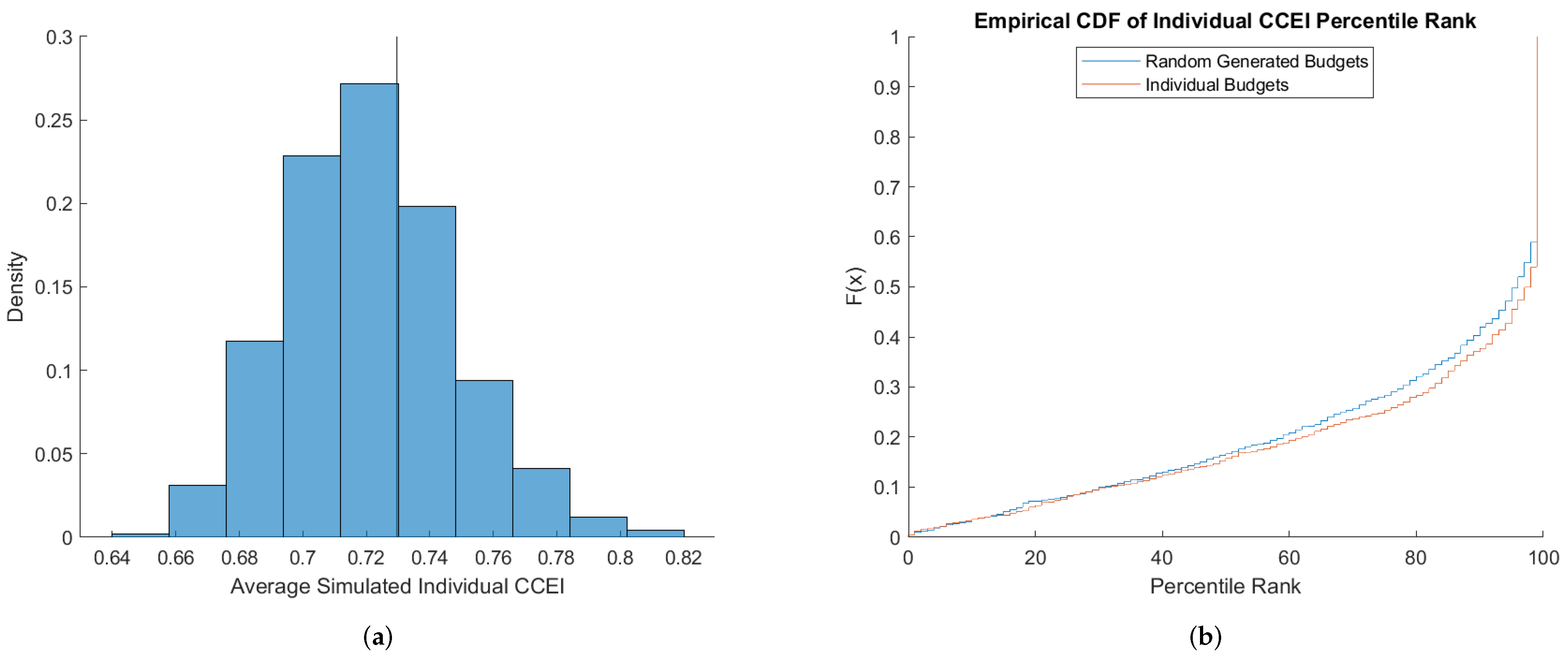
Figure 4 shows how the two benchmarks compare with respect to the CCEI. The histogram in Figure 4a shows that the average CCEIs under the individual budgets benchmark range from 0.64 to 0.82. The distribution of the individual budgets benchmark has more mass below the average CCEI from the random budgets benchmark. This downward bias suggests subjects are slightly more rational than suggested by the random budgets benchmark. This fact is evidenced by the empirical distribution of subject’s percentile ranks in Figure 4b. Percentile ranks under the individual budgets benchmarks are slightly higher on average. The two distributions are significantly different as indicated by a Wilcoxon signed-rank matched pairs test having a p-value .
Figure 5 shows the comparison with respect to HMI. We find qualitatively similar results to those from CFGK. Average HMI under the individual budgets benchmarks range from 17.5 to 21 as shown in Figure 5a. The average of the distribution of the random budgets benchmark is higher than most of the individual budget benchmarks. Thus, on average, the random budget simulations generate fewer violations of GARP. This means that subjects are, on average, more rational than captured by the random budget benchmark. This can also be seen by observing that the percentile ranks of individual subjects with respect to the individual budgets benchmarks first order stochastically dominates the percentiles under the random budgets benchmarks in Figure 5b. The two distributions are significantly different as indicated by a Wilcoxon signed-rank matched pairs test having a p-value . We note that the step function of the random generated budget benchmark occurs here since there is little variation in the HMI across random budgets which leads to a clustering in the percentile ranks.
Correlation with Observable Characteristics
Several revealed preference experiments using random budgets have tried to find correlations between measures of choice consistency and observable socio-economic indicators. For example, Choi et al. [1] establish a relationship between measures of wealth and choice consistency. Cettolin et al. [2] find measures of choice consistency are related to stress. Li et al. [3] compare choice consistency across medical students and the general population. One concern with using the random budgets method when looking for these correlations is that it is possible that observable characteristics might be picking up the random difference of power to reject GARP that results from different budgets. We expect this to be an issue when either there are a small number of budget sets or a small number of individuals. Thus, one should control for this variation when looking for correlations of choice consistency with observable characteristics. Dean and Martin [17] raise a similar point in using raw values for comparing measures of choice consistency. Using household consumption data, they show that accounting for this variation in budgets (by means of the measure of predictive success of [10]) can lead to more pronounced correlations and/or reverse the signs of the relationship.
To check whether the random budget method introduces noise picked up by observable characteristics, we conduct a regression analysis in a similar fashion to that of CMKS. We examine whether a subject’s choice consistency is correlated with their corresponding individual budget benchmark average. We also study whether or not this correlation can affect the relationship between an individual’s socio-economic indicators and choice consistency. We recall that this study has 1182 individuals and 25 budget sets. Thus, we are examining whether 25 random budget sets is enough to ensure the noise from random budgets ability to detect GARP violations is small.
Table 1 shows OLS regression results for CCEI. Omitted categorical variables include: male; ages below 35; low education; household income below €2500; occupation retired; no partner and no children. Column 1 regresses a subject’s CCEI on the average of the simulated CCEIs following the individual budgets benchmark. As expected, we observe a strong positive correlation: the more permissive the budget sets faced by a subject, the higher their CCEI. Column 2 regresses a subject’s CCEI on their socio-economic indicators. Column 3 expands on column 2 by controlling for the simulated CCEIs. We find the same strong positive correlation between an individual’s CCEI and the simulated CCEI. Furthermore, we observe virtually no change in the coefficients for all demographic variables nor in their statistical significance. Coefficients on Female, Age 50–64, Age 65+, High Education, Income €5000+, Housework and Partner all have p-values less than 0.05 in both Columns 2 and 3. This makes sense seeing how the simulated CCEIs are essentially random noise and are thus uncorrelated with any of the demographic indicators.
Table 1 shows OLS regression results for CCEI. Omitted categorical variables include: male; ages below 35; low education; household income below €2500; occupation retired; no partner and no children. Column 1 regresses a subject’s CCEI on the average of the simulated CCEIs following the individual budgets benchmark. As expected, we observe a strong positive correlation: the more permissive the budget sets faced by a subject, the higher their CCEI. Column 2 regresses a subject’s CCEI on their socio-economic indicators. Column 3 expands on column 2 by controlling for the simulated CCEIs. We find the same strong positive correlation between an individual’s CCEI and the simulated CCEI. Furthermore, we observe virtually no change in the coefficients for all demographic variables nor in their statistical significance. Coefficients on Female, Age 50–64, Age 65+, High Education, Income €5000+, Housework and Partner all have p-values less than 0.05 in both Columns 2 and 3. This makes sense seeing how the simulated CCEIs are essentially random noise and are thus uncorrelated with any of the demographic indicators.
Table 2 shows the results using the same regression specifications for HMI. The omitted variables are the same as those in the other regressions. Qualitatively, the results are the same. We observe a strong positive correlation between an individual’s HMI and the simulated average. Furthermore, controlling for the simulated average has no effect on any existing correlation between the HMI and the demographic indicators. Coefficients on Female, Age 50–64, Age 65+, High Education, Paid work, House work, Other and Partner all have p-values less than 0.05 in both Columns 2 and 3.
5. Conclusions
We provide a method to account for the variation in the budget sets when comparing measures of choice consistency across subjects in revealed preference experiments using random budgets and apply this methodology to two existing experimental datasets. Our results suggest that the random budgets method results in a bias when evaluating how rational individual choices appear. We also show that the variation from random budgets does not affect any correlations with demographic variables as predicted by theory.
One thing which is interesting to note is that the average measure of choice consistency from the random budgets benchmark does not fall near the average of the individual budgets benchmark. The reason for this is that while there is a large number of budgets sampled, there is only one choice sampled from each budget. Thus, there is a small sample issue since we are getting a biased sense of the power of each set of budgets drawn. An alternative method which would alleviate this problem is to draw more simulated choices from each set of random budgets. However, we note that this is not the method that has been used in the previous research and would still involve comparing individual choice consistency to the power of budgets that individuals were unlikely to face.
Another thing of note is that some of these issues could be eliminated by changing the method used to generate budgets. For example, an ex-ante random budget method where budgets are randomly drawn according to some criteria ex-ante and that are the same for all individuals would not have this problem. The reason for this is that all individuals would have the same budgets and the power of the test would be guaranteed to be the same. One could filter out situations like that of Figure 1b in the budget selection criteria to improve the power of the random budgets. We note that other papers (see e.g., Andreoni and Miller [21], Andreoni and Harbaugh [22]) have chosen non-randomly budgets ex-ante to be the same across subjects to examine certain comparative statics. We note that the ex-ante random budget method could still facilitate an analysis of comparative statics. For example, the criteria in the ex-ante randomization could first pick a random endowment point, then select five different prices that pivot around the endowment, and finally pick enough endowment points to achieve a power that the researcher deems high enough.
There are a couple of avenues for future research. Firstly, it remains to be seen how sensitive the individual budgets benchmark is to the number of budgets being simulated. Secondly, our benchmark is based on using the method of uniform random sampling Bronars [5] to conduct simulations. Recently, Andreoni et al. [11] develop additional power measures that use the observed choice data to construct the distribution for the data generating process. It is relatively straightforward to incorporate their methodology into our benchmark.
Author Contributions
Both authors have contributed equally to this manuscript. All authors have read and agreed to the published version of the manuscript.
Funding
This research received no external funding.
Institutional Review Board Statement
Not applicable.
Informed Consent Statement
Not applicable.
Data Availability Statement
Restrictions apply to the availability of these data. Data was obtained from the journal repositories and are available at https://0-doi-org.brum.beds.ac.uk/10.1257/aer.97.5.1921 (CFGK) and https://0-doi-org.brum.beds.ac.uk/10.1257/aer.104.6.1518. (CKMS). The code for the analysis is available upon request from the authors.
Acknowledgments
We thank P. J. Healy and three anonymous referees for helpful comments. Any remaining errors are our own. John Rehbeck is supported in part by the National Science Foundation grant NSF-2049749. Opinions, findings, conclusions or recommendations offered here are those of the authors and do not necessarily reflect the views of the National Science Foundation.
Conflicts of Interest
The authors declare no conflict of interest.
References
- Choi, S.; Kariv, S.; Müller, W.; Silverman, D. Who is (more) rational? Am. Econ. Rev. 2014, 104, 1518–1550. [Google Scholar] [CrossRef] [Green Version]
- Cettolin, E.; Dalton, P.S.; Kop, W.; Zhang, W. Cortisol meets GARP: The effect of stress on economic rationality. Exp. Econ. 2019, 23, 554–574. [Google Scholar] [CrossRef] [Green Version]
- Li, J.; Dow, W.H.; Kariv, S. Social preferences of future physicians. Proc. Natl. Acad. Sci. USA 2017, 114, E10291–E10300. [Google Scholar] [CrossRef] [PubMed] [Green Version]
- Choi, S.; Fisman, R.; Gale, D.; Kariv, S. Revealing preferences graphically: An old method gets a new tool kit. Am. Econ. Rev. 2007, 97, 153–158. [Google Scholar] [CrossRef] [Green Version]
- Bronars, S.G. The power of nonparametric tests of preference maximization. Econometrica 1987, 55, 693–698. [Google Scholar] [CrossRef]
- Choi, S.; Fisman, R.; Gale, D.; Kariv, S. Consistency and heterogeneity of individual behavior under uncertainty. Am. Econ. Rev. 2007, 97, 1921–1938. [Google Scholar] [CrossRef] [Green Version]
- Afriat, S.N. The construction of utility functions from expenditure data. Int. Econ. Rev. 1967, 8, 67–77. [Google Scholar] [CrossRef] [Green Version]
- Houtman, M.; Maks, J. Determining all maximal data subsets consistent with revealed preference. Kwant. Methoden 1985, 19, 89–104. [Google Scholar]
- Crawford, I.; De Rock, B. Empirical Revealed Preference. Annu. Rev. Econ. 2014, 6, 503–524. [Google Scholar] [CrossRef] [Green Version]
- Beatty, T.K.; Crawford, I.A. How demanding is the revealed preference approach to demand? Am. Econ. Rev. 2011, 101, 2782–2795. [Google Scholar] [CrossRef] [Green Version]
- Andreoni, J.; Gillen, B.J.; Harbaugh, W.T. The power of revealed preference tests: Ex-post evaluation of experimental design. 2013; unpublished manuscript. [Google Scholar]
- Demuynck, T. Statistical inference for measures of predictive success. Theory Decis. 2015, 79, 689–699. [Google Scholar] [CrossRef] [Green Version]
- Costa-Gomes, M.; Cueva, C.; Gerasimou, G.; Tejiščák, M. Choice, deferral and consistency. Quantitative Economics, forthcoming.
- Varian, H.R. The nonparametric approach to demand analysis. Econometrica 1982, 50, 945–973. [Google Scholar] [CrossRef]
- Varian, H.R. Goodness-of-fit in optimizing models. J. Econom. 1990, 46, 125–140. [Google Scholar] [CrossRef] [Green Version]
- Echenique, F.; Lee, S.; Shum, M. The money pump as a measure of revealed preference violations. J. Political Econ. 2011, 119, 1201–1223. [Google Scholar] [CrossRef] [Green Version]
- Dean, M.; Martin, D. Measuring rationality with the minimum cost of revealed preference violations. Rev. Econ. Stat. 2016, 98, 524–534. [Google Scholar] [CrossRef]
- Demuynck, T.; Rehbeck, J. Computing Revealed Preference Goodness-of-Fit Measures with Integer Programming; Working Paper; ECARES: Brussels, Belgium, 2021. [Google Scholar]
- Murphy, J.H.; Banerjee, S. A caveat for the application of the critical cost efficiency index in induced budget experiments. Exp. Econ. 2015, 18, 356–365. [Google Scholar] [CrossRef]
- Fisman, R.; Jakiela, P.; Kariv, S.; Markovits, D. The distributional preferences of an elite. Science 2015, 349. [Google Scholar] [CrossRef] [PubMed] [Green Version]
- Andreoni, J.; Miller, J. Giving according to GARP: An experimental test of the consistency of preferences for altruism. Econometrica 2002, 70, 737–753. [Google Scholar] [CrossRef] [Green Version]
- Andreoni, J.; Harbaugh, W. Unexpected Utility: Experimental Tests of Five Key Questions about Preferences over Risk; University of Oregon: Eugene, OR, USA, 2009. [Google Scholar]
Figure 1.
Example Budget Sets. (a) Set 1, (b) Set 2.

Figure 2.
Simulation results for CCEI (CFGK). (a) Histogram, (b) Percentile Ranks.

Figure 3.
Simulation results for HMI (CFGK). (a) Histogram, (b) Percentile Ranks.

Figure 4.
Simulation results for CCEI (CKMS). (a) Histogram, (b) Percentile Ranks.

Figure 5.
Simulation Results for HMI (CKMS). (a) Histogram, (b) Percentile Ranks.


Table 1.
Regressions with CCEI.
| (1) | (2) | (3) | |
|---|---|---|---|
| CCEI | CCEI | CCEI | |
| Sim CCEI Avg | 0.38 | 0.39 | |
| (0.15) | (0.15) | ||
| Female | −0.024 | −0.024 | |
| (0.0089) | (0.0089) | ||
| Age 35–49 | −0.016 | −0.017 | |
| (0.011) | (0.011) | ||
| Age 50–64 | −0.052 | −0.053 | |
| (0.011) | (0.011) | ||
| Age 65+ | −0.052 | −0.054 | |
| (0.020) | (0.020) | ||
| Medium education | 0.0090 | 0.0086 | |
| (0.011) | (0.011) | ||
| High education | 0.026 | 0.026 | |
| (0.011) | (0.011) | ||
| Income 2500–3499 | 0.026 | 0.025 | |
| (0.012) | (0.012) | ||
| Income 3500–4999 | 0.020 | 0.020 | |
| (0.013) | (0.013) | ||
| Income 5000+ | 0.033 | 0.033 | |
| (0.014) | (0.014) | ||
| Paid work | 0.028 | 0.027 | |
| (0.018) | (0.018) | ||
| House work | 0.046 | 0.045 | |
| (0.021) | (0.021) | ||
| Other | 0.037 | 0.036 | |
| (0.019) | (0.019) | ||
| Partner | −0.026 | −0.026 | |
| (0.011) | (0.011) | ||
| # Children | 0.00069 | 0.00039 | |
| (0.0042) | (0.0042) | ||
| Constant | 0.61 | 0.89 | 0.61 |
| (0.11) | (0.022) | (0.11) | |
| Observations | 1182 | 1182 | 1182 |
| Adjusted | 0.00 | 0.06 | 0.06 |
Robust standard errors in parentheses.
Table 2.
Regressions with HMI.
| (1) | (2) | (3) | |
|---|---|---|---|
| HMI | HMI | HMI | |
| Sim HMI Avg | 0.50 | 0.47 | |
| (0.17) | (0.16) | ||
| Female | −0.39 | −0.37 | |
| (0.14) | (0.14) | ||
| Age 35–49 | −0.28 | −0.27 | |
| (0.20) | (0.20) | ||
| Age 50–64 | −0.93 | −0.91 | |
| (0.19) | (0.19) | ||
| Age 65+ | −0.75 | −0.71 | |
| (0.31) | (0.31) | ||
| Medium education | 0.31 | 0.33 | |
| (0.17) | (0.17) | ||
| High education | 0.69 | 0.72 | |
| (0.18) | (0.18) | ||
| Income 2500–3499 | 0.19 | 0.20 | |
| (0.19) | (0.19) | ||
| Income 3500–4999 | 0.11 | 0.097 | |
| (0.20) | (0.20) | ||
| Income 5000+ | 0.28 | 0.25 | |
| (0.22) | (0.21) | ||
| Paid work | 0.62 | 0.62 | |
| (0.27) | (0.27) | ||
| House work | 0.98 | 0.96 | |
| (0.31) | (0.31) | ||
| Other | 0.86 | 0.90 | |
| (0.29) | (0.29) | ||
| Partner | −0.39 | −0.36 | |
| (0.18) | (0.18) | ||
| # Children | −0.023 | −0.024 | |
| (0.070) | (0.070) | ||
| Constant | 12.6 | 22.2 | 13.1 |
| (3.20) | (0.36) | (3.18) | |
| Observations | 1182 | 1182 | 1182 |
| Adjusted | 0.01 | 0.07 | 0.07 |
Robust standard errors in parentheses.
Publisher’s Note: MDPI stays neutral with regard to jurisdictional claims in published maps and institutional affiliations. |
© 2022 by the authors. Licensee MDPI, Basel, Switzerland. This article is an open access article distributed under the terms and conditions of the Creative Commons Attribution (CC BY) license (https://creativecommons.org/licenses/by/4.0/).
Share and Cite
MDPI and ACS Style
Mahmood, M.A.; Rehbeck, J. Correcting for Random Budgets in Revealed Preference Experiments. Games 2022, 13, 30. https://0-doi-org.brum.beds.ac.uk/10.3390/g13020030
AMA Style
Mahmood MA, Rehbeck J. Correcting for Random Budgets in Revealed Preference Experiments. Games. 2022; 13(2):30. https://0-doi-org.brum.beds.ac.uk/10.3390/g13020030
Chicago/Turabian StyleMahmood, Mir Adnan, and John Rehbeck. 2022. "Correcting for Random Budgets in Revealed Preference Experiments" Games 13, no. 2: 30. https://0-doi-org.brum.beds.ac.uk/10.3390/g13020030
Note that from the first issue of 2016, this journal uses article numbers instead of page numbers. See further details here.