Imitation Dynamics in Oligopoly Games with Heterogeneous Players

Abstract

We investigate the role and performance of imitative behavior in a class of quantity-setting, Cournot games. Within a framework of evolutionary competition between rational, myopic best-response and imitation heuristics with differential heuristics’ costs, we found that the equilibrium stability depends on the sign of the cost differential between the unstable heuristic (Cournot best-response) and the stable one (imitation) and on the intensity of the evolutionary pressure. When this cost differential is positive (i.e., imitation is relatively cheaper vis a vis Cournot), most firms use this heuristic and the Cournot equilibrium is stabilized for market sizes for which it was unstable under Cournot homogeneous learning. However, as the number of firms increases $(n=7)$, instability eventually sets in. When the cost differential is negative (imitation is more expensive than Cournot), complicated quantity fluctuations, along with the co-existence of heuristics, arise already for the triopoly game.

1. Introduction

Ref. [1] remarkably shows that, when firms compete on quantity using the [2] adjustment process1, the Cournot-Nash equilibrium becomes unstable if the number of firms exceeds two. In fact, with linear demand and constant marginal costs, the Cournot-Nash equilibrium loses stability and bounded but perpetual oscillations arise already for a triopoly. For more than three firms oscillations grow unbounded, but they are limited once the non-negativity price and demand constraints bind.

Whereas [1] focused only on the homogeneous (Cournot) adjustment process, more recent research extends to models of heterogeneous expectations2. For instance, Ref. [3] focus on the Cournot heuristic in competition with rational firms, under replicator dynamics. Ref. [4] extend the framework in which these heuristics compete in a quantity-setting oligopoly with arbitrary number of firms and for general monotone selection dynamics. Each firm chooses a behavioral rule from a finite set of different rules, which are assumed to be commonly known. When making a choice concerning the behavioral rules, a firm takes the past performance of the rules, i.e., the past realized profit net of the cost associated with the behavioral rules to compare fitness. Both past performance and costs associated with the behavioral rules are publicly available. This implies that successful heuristics will continue to be used, while unsuccessful behavioral rules are dropped.

Experimental evidence for the (in)stability and homogeneous learning in Cournot games, even in linear environments, is rather mixed. Ref. [5] discuss a linear Cournot oligopoly experiment with four firms. They do not find that quantities explode as the [1] model predicts, instead the time average quantities converge to the Cournot-Nash equilibrium quantity, although there is substantial volatility of the actual period-by-period around the Cournot-Nash equilibrium quantity. Ref. [6] run laboratory experiments on two types of linear Cournot oligopolies, the one that displays an unique, stable interior Nash equilibrium (Type I) and a Type II oligopoly for which the interior equilibrium is unstable and two additional, stable boundary Nash equilibria emerge (with one firm acting as a de facto monopolist). Subjects learn to play the Type I, interior stable equilibrium, but not the unstable, or even the stable, boundary ones in the Type II oligopoly. Importantly, on the equilibration path, they reject prediction of homogeneous learning theories such as Cournot adjustment, fictitious play or best-reply to the average of opponents’ entire past play3. The experimental rejection of the homogeneous learning theories above, naturally leads us to consider alternative heuristics and, more generally, heterogenous learning, with rules updating.

Among the alternative heuristics, there is an increasing interest, both theoretical and experimental, in understanding the performance of imitative players. Ref. [8] show that Cournot markets with players imitating the past successful strategy of their opponents converge to the Walrasian equilibrium. However, the hypothesis that players actually use the imitate-the-best heuristics in Counot games is invalidated, experimentally, by [9]. They posit that (naive) imitate-the-best players may realize that past period “success” may be purely drive by a particular realization of opponents’ types. Ref. [10] adds myopic optimizers (Cournot best-responders) to [8] population of imitate-the-best players, and finds that in stationary distribution of the stochastic process, the imitators are better off. Moreover, Ref. [11] prove that imitation can be unbeatable if imitate-the-best heuristic is not subjected to a money pump (i.e., game is not of the circular best-reply, Rock-Scissors-Paper type). Subsequently, Ref. [12] show that unconditional imitation, of the tit-for-tat variety, is essentially unbeatable in class of potential games. Ref. [13] analyze a Cournot duopoly, subjects earn on average higher profits when playing against “best-response” computers than against “imitate-the-successful” computers. Ref. [5] find that a process where participants mix between the Cournot adjustment heuristic an imitating the previous period’s average quantity gives the best description of behavior. Our choice of modelling imitation as imitate-the-average lagged strategy in the population is informed, on the one hand, by this experimental result, and, on the other hand, by the evidence against imitate-the-most successful past period strategy in [9]. The imitate-the-average heuristic will be tested, firstly, against the standard Cournot heuristic, i.e., firms best-respond to average population past play, and secondly, against ‘rational’ players, i.e., players that understand that they are facing a distribution of updating players types (heuristics) and, consequently, they respond optimally to the expected configuration of types in the market. We show that, even if the imitate-the-average tends to stabilize the Cournot equilibrium (the thresholds for which instability sets in is typically higher, ceteris paribus, in comparison to models of heterogeneous learning without imitation), the differential costs of the more sophisticated heuristic over the simpler one rest critical for the instability threshold number of players, as well as for the non-equilibrium dynamics around Cournot-Nash equilibrium.

Outside the oligopoly realm, learning rules evolution has also been investigated in two-person, strategic games. Ref. [14] look at the interplay of three heuristics—best-response, imitate-the-majority, imitate-the-minority—and show that it may generate complex, non-Nash equilibrium attractors, such as limit cycles, even in simple, $2\times 2$ Coordination games. Ref. [15] finds that, in a coordination game with endogenous updating of myopic best-response imitate-the best heuristic, the efficient equilibrium is selected. Ref. [16] also considers $2\times 2$ coordination games, but with a threewise ecology of best-reply, better-reply and imitate-the best action among the sample of past play and prove that the risk-dominant equilibrium is selected for small sample sizes. Ref. [17] studies the evolution of bargaining rules (i.e., pie-sharing demands rules) via an external stability argument, by which incumbent rules should do better than mutant demands, reminiscent of the concept of ESS of [18]. To this rule evolution literature, we contribute the study of a threewise ecology of heuristics—naive best-reply, equilibrium (rational) play and imitate-the-average past play—which, to the best of our knowledge, has not been investigated before. It would be a direct exercise to apply our methodology to the simple $2\times 2$ coordination games that the previous work on heterogenous learning rules has focused on.

A somewhat parallel stream of literature deals with the evolution of preferences4 as the underlying factor upon which selection acts and which, in turns determines the actual strategy choice in the game played. Pioneered by [19], who shows that utility-maximization (homo economicus) may be just one among many preferences types selected by evolution in the quest of adaptation to environment, this “indirect evolutionary approach” was developed further in the context of two-person games by, e.g., [20,21]. They look at stable configurations of preferences-game equilibria and document the striking possibility that non-Nash outcomes and non-maximizing preferences can be stable, evolutionarily. In the IO literature, Ref. [22] use this indirect approach to show that owners’ preferences overs managers’ incentives do not always converge to profit-maximization, but may favor sales maximization, in Cournot competition or even sales minimization, in differentiated Bertrand oligopolies. Relatedly, Ref. [23] prove that oligopolists’ preferences may evolve towards total surplus (producer and consumer) maximization, rather than the (narrow) profit-maximization, assumed by the rational producer theory.

Our approach is largely driven by the quest for understanding the behaviour of boundedly rational players, disciplined by the evolutionary selection operating at the level of behavioral rules. In particular, the question of whether learning converges to the Counot equilibrium, in an environment with competing and costly learning rules. Therefore, we put forth, three ecologies of heterogeneous heuristics (Cournot vs. Imitation, Rational vs. Imitation, Rational vs. Cournot vs. Imitation). Both the fixed fractions and evolutionary switching between heuristics scenarios, are discussed. Our concern is, first and foremost, the role and performance of the imitate-the-average heuristic within a given menu of heuristics, and, secondly, if for a given configuration of heuristics, the Cournot-Nash equilibrium is (un)stable. Unlike, for instance, Ref. [10], our imitate-the-average rule does not always outperforms Cournot, or sophisticated (rational) play, but may co-exist with other heuristics in equilibrium. In contrast to the strong convergence result in [8], complicated, non-Cournotian equilibrium limit sets (two-cycles, strange attractors) may emerge once learning heterogeneity is endogenized.

Main findings are that, first, the stability of Cournot equilibrium critically depends on the cost advantage of the ‘stable’ heuristic (imitation) vis-a-vis the unstable one (Cournot myopic best-reply): when the (relatively) cheaper behavioral rule is imitation, the dynamics converge to a situation where most firms use this behavioral rule and all firms produce the Cournot-Nash equilibrium quantity, for market sizes for which homogeneous Cournot play is known to destabilize the interior equilibrium (e.g., triopoly). However, instability eventually sets in, if the number of firms passes a higher threshold $(n=7)$. In the case when the relatively cheaper heuristic is unstable, complicated endogenous fluctuations may already occur for $n=3,$ in particular, when the evolutionary pressure is high. The nonlinearity causing this erratic behavior comes from the endogenously updating of the fractions, because in our leading example the oligopoly specifications were linear. Secondly, when rational firms compete with imitators, in the particular scenario of linear inverse demand and constant marginal cost, the system is always stable regardless of the game and behavioral parameters. Last, in the case when rational firms, Cournot firms and imitators compete, the stability depends on the differential cost of the rational plays versus the Cournot and imitation heuristics, as well as on the magnitude of the evolutionary pressure. For very large intensity of selection ($\beta \to \infty )$ and for costly rational choice and costless Cournot and imitation rules, we are able to recover analytically the $n=7$ instability threshold in the pairwise contest Cournot vs. imitation.

The remainder of this paper is organized as follows, in Section 2 the theoretical framework is introduced, namely the quantity-setting oligopoly, the menu of heuristics and the population evolutionary dynamics. In Section 3 the evolutionary dynamics will be investigated under exogenous population fractions whereas in Section 4 the stability of systems made of two learning rules will be investigated, under endogenous population dynamics. In Section 5 the model extended to a three heuristics environment, with rational players, Cournot and imitators competing and switching learning heuristics, according to their relative performance. Finally, we conclude in Section 6.

2. Set-Up

Consider a finite population of firms who are competing on the market for a certain good, each discrete-time period all producers have to decide their production plans for the next period. However, instead of simultaneously choosing the supplied quantities directly, the firms act according to behavioral rules that exactly prescribe the quantity to be supplied. Before the evolutionary model is studied a brief review of the traditional, static Cournot model will be given.

Consider a symmetric Cournot oligopoly game, where $q_i$ denotes the quantity supplied by firm $i, \mathrm{where}i=1,\dots n$. Next to that let $Q={\sum }_{i=1}^n{q}_i$ be the aggregated production. Furthermore let $P\left(Q\right)$ denote the twice differentiable, nonnegative and non-increasing inverse demand function and let $C\left(q_i\right)$ denote the twice differentiable non-decreasing cost function, which is the same for all firms. For firm i the resulting profit function from the above described model is given by

$${\pi }_i(q_i,Q_{-i})=P(q_i+Q_{-i})q_i-C\left(q_i\right),i=1,\dots n$$

(1)

where $Q_{-i}={\sum }_{j\ne i}{q}_j$. Assume that the profit function of a firm is strictly concave in its own output $q_i$. The profit maximizing strategy of firm i, taking the quantity supplied by the competitors as given, results in the well-known best-reply function for firm i, which is given by

$$q_i=R_i\left(Q_{-i}\right)=\underset{q_i}{Argmax}[P(q_i+Q_{-i})q_i-C\left(q_i\right)].$$

Due to symmetry, all firms have the same best-reply function $R(·)$. Moreover, the symmetric Cournot-Nash equilibrium quantity $q^{*}$ corresponds to the solution of

$$q^{*}=R\left((n-1)q^{*}\right).$$

In the sequel, we will restrict the analysis to oligopolies displaying an unique, interior Nash equilibrium, the so called Type I oligopoly in [6]5. This very general class includes, as special cases, oligopolies with linear demand and (i) constant, (ii) increasing and (iii) even decreasing marginal costs, as long as marginal costs do not decrease too fast, compared to the demand function. In Type I duopolies most learning processes (Cournot best-reply, adaptive dynamics, fictititous play, etc) are known to converge to the unique, interior fixed point. This is not the case for the Type II duopolies6. It is the main reason why we focus on the Type I oligopolies, as we want to isolate the instability built into the the oligopoly game itself from the destabilizing forces that reside in the heuristics’ of choice and their updating mechanism.

The original Cournot specification of [1] falls within the class of Type I oligopoly and will be used as leading example: an oligopoly game with linear inverse demand and linear costs, given by

$$P(q_i+Q_{-i})=a-b(q_i+Q_{-i})\mathrm{and}C\left(q_i\right)=c{q}_i,i=1,\dots n$$

respectively. First, in order to have a strictly concave profit function assume that $b>0$. Furthermore, for strictly positive prices we assume that $q_i<\frac{a}{nb}$ (so that aggregate output $Q<\frac{a}{b}$ and $P\left(Q\right)>0)$. For these specifications of the inverse demand function and cost function the reaction function is given by

$$q_i=R\left(Q_{-i}\right)=\frac{a-c}{2b}-\frac{1}{2}{Q}_{-i}=q^{*}-\frac{1}{2}(Q_{-i}-(n-1)q^{*}).$$

(2)

Note that if the other firms produce on average more (less) than the Cournot-Nash equilibrium quantity, firm i reacts by producing less (more) than that quantity.

Straightforward calculations show that in this case the Cournot-Nash equilibrium quantity, aggregated production, price and profit are equal to $q^{*}=\frac{a-c}{b(n+1)}$, $Q^{*}=\frac{a-c}{b}\frac{n}{n+1}$, $P^{*}=\frac{a+nc}{n+1}\mathrm{and}{\pi }^{*}=\pi (q_i^{*},Q_{-i}^{*})=\frac{{(a-c)}^2}{b{(n+1)}^2}$.

Traditional Cournot analysis refers to a static environment. However, in a dynamic setting the reaction function introduced above can be used to study the so called Cournot-dynamics where firms best-reply to their expectations

$$q_{i,t}=R\left(Q_{-i,t}^e\right),i=1,\dots n$$

where $q_{i,t}$ denotes the quantity supplied by player i in period t and $Q_{-i,t}^e$ stands for player’s i expectations about her opponents’s total output at time t. The symmetric Cournot-Nash equilibrium where all firms produce $q^{*}$ is stable under the Cournot-dynamics if $(n-1)|R^{\prime *}\left)\right|<1$.

Main interest is on how firm i decides to play $q^{*}$ and, more specifically, what does firm i believe about $Q_{-i}$ when the production decision has to be made. Our key assumption is that firms are choosing their expectation-formation rule (heuristic) based on its performance.

2.1. Learning Heuristics

In the Cournot oligopoly game the producers have to form expectations about opponents’ production plans. Based on this expectation firms decide how much to produce the next period. One approach is to assume complete information, i.e., rational firms with common knowledge of rationality. This implies that firms have perfect foresight about competitors’ aggregated production plan, i.e., $Q_{-i,t+1}^e=Q_{-i,t+1}.$ This results in the following production plan:

$$q_{i,t+1}=R\left(Q_{-i,t+1}\right),i=1,\dots n.$$

Alternatively one may consider rules that require less information, for example $Q_{-i,t+1}^e=Q_{-i,t}.$ This results in the following production plan:

$$q_{i,t+1}=R\left(Q_{-i,t}\right),i=1,\dots n$$

(3)

where firms expect that aggregated production in the next period equals current aggregated production. This is the so called Cournot adjustment heuristic. It is an straightforward exercice to show that, if all firms use the Cournot heuristic, the Cournot-Nash equilibrium is a locally asymptotically stable7 fixed point of system (3) whenever

$$\lambda \left(n\right)\equiv (n-1)\left|R^{\prime *}\right|<1,$$

(4)

where $\lambda \left(n\right)$ is defined as the largest eigenvalue of the Jacobian, evaluated at the equilibrium.

Leading example. From Equation (2) it can easily be seen that $R^{\prime }\left(Q_{-i}^{*}\right)=-\frac{1}{2}$, meaning that if others’ aggregated output increases by one unit, the Cournot-Nash firms decrease their output by $\frac{1}{2}$ units. From stability condition (4) it follows that the Cournot-Nash equilibrium is stable for this specification only when $n=2$ and unstable when $n>3$ (and neutrally stable, resulting in bounded oscillations, for $n=3$). The reason for this instability is ‘overshooting’: if aggregated output is above (below) the Cournot-Nash equilibrium quantity, firms react by reducing (increasing) their output. For $n>3$ this aggregated reduction (increase) in output is so large that the resulting deviation of aggregated output from the equilibrium quantity is larger in the next period than in the current, and so on.

It is a broadly supported idea that not all producers best-reply to their expectations. Experiments [5] show that people often imitate others’ behavior. A heuristic that possibly seizes this production plan is the so called imitation-the-average heuristic. Imitators believe that “everyone else can’t be wrong” and will therefore produce the average of the other players’ production in the next period, i.e.,

$$q_{i,t+1}=\frac{Q_{-i,t}}{n-1},i=1,\dots ,n.$$

(5)

Local stability of the Cournot-Nash equilibrium with only imitation firms depends on the eigenvalues of the Jacobian matrix of the system of Equation (5) evaluated at that Cournot-Nash equilibrium $q^{*}$. This Jacobian matrix is given by

$${\left.J\right|}_{q^{*}}=\left(\begin{array}{cccc}0& \frac{1}{n-1}& \cdots & \frac{1}{n-1}\\ \frac{1}{n-1}& 0& & ⋮\\ ⋮& & \ddots & \frac{1}{n-1}\\ \frac{1}{n-1}& \cdots & \frac{1}{n-1}& 0\end{array}\right).$$

(6)

Imitators only respond to other firms’ production and do not respond to their own production, therefore all diagonal elements are equal to zero. If one competitor increases current production by one unit, an imitator will increase next production with $\frac{1}{n-1}$ unit, therefore all off-diagonal elements are equal to $\frac{1}{n-1}$. The Jacobian matrix (6) thus has $n-1$ eigenvalues equal to $-\frac{1}{n-1}$ and one eigenvalue equal to $(n-1)\frac{1}{n-1}=1$ which is the largest in absolute value. Therefore it follows immediately that the Cournot-Nash equilibrium is neutrally stable independent of n and game structure (demand and cost function). The reason for this is that if one producer changes his production plan the economy will stabilize to a new equilibrium unequal to $q^{*}$ and will remain at this new equilibrium until one producer deviates again. In fact this system has infinitely many neutrally stable equilibria, namely if $q_i=q^{†}\forall i,$ the system is neutrally stable for all $q^{†}.$

2.2. Population Dynamics

In the previous section it was shown how the supplied quantities evolve over time under the Cournot and the imitation heuristic. In this section it will be explained how the population fractions evolve over time. Let us first introduce the vector ${\eta }_t$ which has entries equal to ${\eta }_{k,t}$, which is the fraction of the population that uses heuristic k at time t. Thus for every time t, ${\eta }_t$ denotes the K-dimensional vector of fractions for each strategy/heuristic and belongs to the K-dimensional simplex ${\Delta }^K=\{{\eta }_t\in {\mathbb{R}}^K:{\sum }_{k=1}^K{\eta }_{k,t}=1;0\le {\eta }_{k,t}\le 1\forall k\}$. We will now describe how the fractions ${\eta }_{k,t}$ evolve over time. It is assumed that the choice of a behavioral rule is based on its past performance, capturing the idea that more successful rules will be used more frequently.

Evolutionary game theory deals with games played within a (large) population over a long time horizon. Its main ingredients are its underlying game, e.g., the Cournot one-shot game, and the evolutionary dynamic class which defines a dynamical system on the state of the population. The evolutionary dynamical system depends on current fractions ${\eta }_t$ and current fitness $U_t$. In general, such an evolutionary dynamic in discrete time, describing how the population fractions evolve, is given by

$${\eta }_{k,t+1}=K(U_t,{\eta }_t)$$

(7)

with $U_t={(U_{1,t},\dots ,U_{K,t})}^{\prime }$ the vector of average utilities and ${\eta }_t={({\eta }_{1,t},\dots ,{\eta }_{K,t})}^{\prime }$ the factor of fractions. To make sure that the population dynamics is well-behaved in terms of dynamic implications we assume that $K(·,·)$ is continuous, nondecreasing in $U_{k,t}$, and such that the population state remains in the K-dimensional unit simplex ${\Delta }^K$. One widely used evolutionary dynamic in the literature on learning in games is the Logit Dynamics (see, e.g., [26] for an extensive treatment). It can be derived from discrete choice/random utility models and it specifies that fractions of different heuristics are updated according to

$${\eta }_{k,t+1}=\frac{e^{\beta U_{k,t}}}{{\displaystyle \sum _{j=1}^K{e}^{\beta U_{j,t}}}},k=1,\dots ,K.$$

(8)

The parameter $\beta$ represents the intensity of selection, and it captures the idea of boundedly rational play, since individuals do not necessarily select the rule that yields the highest utility. Notice that in the extreme case where $\beta =0$ we have completely random behavior: the noise is so large that observed average utility is equal for all behavioral rules. Each behavioral rule is thus chosen with equal probability: ${\eta }_{k,t}=\frac{1}{K}\forall k$. In the other extreme case, when $\beta \to \infty$, everybody switches to the most profitable strategy each period8.

In case of equal costs of the heuristics, equilibrium fractions are thus given by ${\eta }_k^{*}=\frac{1}{K}\forall k$, since production is equal and thus profits are equal.

In the leading examples we will focus on the Logit evolutionary dynamics. Firstly, because the Logit rule is a standard tool in economics for modelling boundedly rational choice, and, secondly, because it displays nice regularity/continuity conditions $(0\le {\eta }_k\le 1)$.

3. Heterogeneity in Behavior in Cournot Oligopolies

In this Section we introduce heterogeneity in production decision’ heuristics. In a population game set-up, n firms are randomly picked, from a large population of firms in which a fraction ${\eta }_k$ plays according to heuristic k. We first focus on pairwise competition between two heuristics, Cournot vs. Imitation and Rational vs. Imitation, respectively, under the no switching scenario. The assumption of fixed shares $\eta$ for each period will be relaxed in Section 4.

3.1. Cournot vs. Imitation Firms with Fixed Fractions

In order to facilitate studying the aggregate behavior of a heterogeneous set of interacting quantity-setting-heuristics we study the Cournot model as a population game. Consider a large population of firms from which in each period groups of n firms are sampled randomly and matched to play the one-shot n-player Cournot game. We assume that a fixed fraction of $\eta$ of the large population of firms uses the Cournot heuristic and the others use the imitation heuristic. After each one-shot Cournot game, the random matching procedure is repeated, leading to new combinations types of firms. The distribution of possible samples follows a binomial distribution with parameters $n,$ and $\eta$. Below the example Cournot vs. Imitation firms will be discussed again but now under the assumption of random matching.

Suppose that a fraction of $\eta$ of the population of the firms uses the Cournot heuristic and observes the population-wide average quantity ${\overline{q}}_t$ and best responds to it, $q_{t+1}^C=R\left((n-1){\overline{q}}_t\right)$, where $q_t^C$ is the quantity produced by each Cournot firm in period t. Consequently a fraction of $\eta$ firms of the large population makes use of the the imitation heuristic. Making use of the law of large numbers, the average quantity played in period t can be expressed as

$${\overline{q}}_t=\eta q_t^C+(1-\eta )q_t^I.$$

Recall that imitate-the-average firms produce, in the next period, the other firms’ average quantity, produced in the current period $q_{i,t+1}^I=\frac{Q_{-i,t}}{n-1}$. Again, by a law of large numbers we obtain $\frac{Q_{-i,t}}{n-1}\to {\overline{q}}_t\mathrm{when}n\to \infty$. Therefore we obtain the following quantity dynamics

$$\begin{array}{cc}\hfill q_{t+1}^C& =R\left((n-1)(\eta q_t^C+(1-\eta )q_t^I)\right)\hfill \\ \hfill q_{t+1}^I& =\eta q_t^C+(1-\eta )q_t^I.\hfill \end{array}$$

(9)

Note that this is a 2-dimensional dynamical system which dimension cannot be reduced. Furthermore the Cournot-Nash equilibrium is not the unique equilibrium of the homogeneous, imitation rule, in fact all quantities are. The Cournot-Nash equilibrium is, however, still the unique equilibrium quantity of the heterogeneous heuristics dynamical system (9).

Proposition 1.

The Cournot-Nash equilibrium, where all firms produce the Cournot-Nash quantity $(q^{*},q^{*})$, is a locally stable fixed point for the model with exogenous fractions of Cournot and imitation firms if and only if

$$|1-\eta +\eta (n-1)\left(R^{\prime *}\right)|<1.$$

(10)

Proof. 

It can easily be shown that the Jacobian matrix, evaluated at the Cournot-Nash equilibrium $(q^{*},q^{*})$, is given by

$$\left(\begin{array}{cc}(n-1)\eta R^{\prime *}& (n-1)(1-\eta )R^{\prime *}\\ \eta & 1-\eta \end{array}\right).$$

(11)

The corresponding eigenvalues are ${\lambda }_1=0$ and ${\lambda }_2=1-\eta +\eta (n-1)R^{\prime *}$. Here ${\lambda }_2$ is the largest eigenvalue in absolute value. Thus the system is stable if $|{\lambda }_2|\hspace{0.17em}<1$, this is the condition stated in the proposition. □

Leading example. Here $R^{\prime *}=-\frac{1}{2}$ substituting this in Equation (10) gives, after some simplification

$$n<\frac{4-\eta }{\eta }.$$

(12)

Meaning that an economy with as much Cournot firms as imitators $(\eta =\frac{1}{2})$ is stable if $n<7$. Next to that as found earlier, an economy with only Cournot firms $(\eta =1)$ is stable if $n<3$. Furthermore, an economy where close to all firms use the imitation heuristic, but some Cournot firms exist ($\eta$ close to zero), the economy is always stable.

3.2. Rational vs. Imitation Firms with Fixed Fractions

In this section we focus on the dynamics when there is competition between rational and imitation firms. We set the fraction of rational firms equal to $\eta$. A fully rational firm is assumed to know the fraction of imitation firms. Moreover, it knows exactly how much all firms will produce. However, we assume that it does not know the composition of firms in its market (or has to make a production decision before observing this). The rational quantity dynamics therefore have the following structure

$$q^R=\underset{q_i}{Argmax}E[P(q_i+Q_{-i})q_i-C\left(q_i\right)].$$

It forms expectations over all possible mixtures of heuristics resulting from randomly drawing $n-1$ other players from a large population, of which each with chance $\eta$ is a rational firm too, and with chance $1-\eta$ is an imitator. Rational firm i therefore chooses quantity $q_i$ such that his objective function, its own expected utility

$$U_t^R\left(q_{i,t}\right|q_t^R,q_t^I,\eta )={\sum }_{k=0}^{n-1}\left(\genfrac{}{}{0.0pt}{}{n-1}{k}\right){\eta }^k{(1-\eta )}^{n-1-k}[P((n-1-k)q_t^I+k{q}_t^R+q_{t,i})q_{t,i}-C\left(q_{t,i}\right)],$$

(13)

is maximized given the production of the other players and the population fractions. Here $q_t^R$ is the symmetric output level of all of the other rational firms in period t, and $q_t^I$ is the output level of all of the imitation firms. The first order condition for an optimum is characterized by equality between marginal cost an expected marginal revenue. Typically, marginal revenue in the realized market will differ from marginal costs.

Given the value of $q_t^I$ and the fraction $\eta$, all rational firms coordinate on the same output level $q_t^R$. This gives the first order condition

$$\frac{\delta U_t^R\left(q_{i,t}\right|q_t^R,q_t^I,\eta )}{\delta q_{i,t}}=0,$$

which equals to:

$$\begin{array}{c}\sum _{k=0}^{n-1}\left(\genfrac{}{}{0.0pt}{}{n-1}{k}\right){\eta }^k{(1-\eta )}^{n-1-k}\times \\ \left[P\right((n-1-k)q_t^I+(k+1)q_t^R)+q_t^R{P}^{\prime }((n-1-k)q_t^I+(k+1)q_t^R)-C^{\prime }\left(q_t^R\right)]=0.\end{array}$$

(14)

Let the solution9 to Equation (14), the rational play quantity be given by $q_t^R=H^R(q_t^I,\eta )$, the full system of equations is thus given by

$$\begin{array}{cc}\hfill q_{t+1}^R& =H^R(q_{t+1}^I,\eta )=H^R(\eta q_t^R+(1-\eta )q_t^I,\eta )\hfill \\ \hfill q_{t+1}^I& =\eta q_t^R+(1-\eta )q_t^I.\hfill \end{array}$$

(15)

It is easily checked that if the imitators play the Cournot-Nash equilibrium quantity $q^{*}$, or if all firms are rational, the rational firms will play the Cournot-Nash equilibrium quantity, that is $H^R(q^{*},\eta )=q^{*}$, for all $\eta$ and $H^R(q^I,1)=q^{*}$ for all $q^I$. Moreover, if a rational firm is certain it will only meet imitation firms (that is $\eta =0$), it plays a best response to the currently average played quantity, that is $H^R(q_t^I,0)=R\left((n-1)q_t^I\right)$, for all $q_t^I$. In the remainder we will denote the partial derivatives of $H^R(q,\eta )$ with respect to q and $\eta$ by $H_q^R(q,\eta )$ and $H_{\eta }^R(q,\eta )$ respectively.

Proposition 2.

The Cournot-Nash equilibrium, where all firms produce the Cournot-Nash quantity $(q^{*},q^{*})$, is a locally stable fixed point for the model with exogenous fractions of rational and imitation firms if and only if

$$|\eta H_q(q*,\eta )+1-\eta |<1.$$

(16)

Proof. 

In order to determine the local stability of the equilibrium $(q^{*},q^{*})$ where all firms produce the Cournot-Nash quantity, we need to determine the eigenvalues of the Jacobian matrix of system (15), evaluated at the equilibrium. It can be shown that this Jacobian matrix is given by

$${\left.J\right|}_{q^{*},q^{*}}=\left(\begin{array}{cc}\eta H_q(q^{*},\eta )& (1-\eta )H_q(q^{*},\eta )\\ \eta & 1-\eta \end{array}\right),$$

(17)

which has eigenvalues ${\lambda }_1=\eta H_q(q^{*},\eta )+1-\eta$ and ${\lambda }_2=0$. Consequently the system is locally stable when $|{\lambda }_1|\hspace{0.17em}<1$, this is exactly the condition stated. □

Leading example. In the leading example the implicit function defining $q_t^R$ (Equation (14)) when using that

$$\sum _{k=0}^{n-1}\left(\genfrac{}{}{0.0pt}{}{n-1}{k}\right){\eta }^k{(1-\eta )}^{n-1-k}=1\mathrm{and}\sum _{k=0}^{n-1}\left(\genfrac{}{}{0.0pt}{}{n-1}{k}\right){\eta }^k{(1-\eta )}^{n-1-k}k=(n-1)\eta$$

boils down to

$$q_{t+1}^R=H^R(q_{t+1}^I,\eta )=\frac{a-c}{b(2+(n-1\left)\eta \right)}-\frac{(n-1)(1-\eta )}{2+(n-1)\eta }(\eta q_t^R+(1-\eta )q_t^I).$$

The system of equations for the leading example is given by

$$\begin{array}{cc}\hfill q_{t+1}^R& =H^R(q_{t+1}^I,\eta )=\frac{a-c}{b(2+(n-1\left)\eta \right)}-\frac{(n-1)(1-\eta )}{2+(n-1)\eta }(\eta q_t^R+(1-\eta )q_t^I)\hfill \\ \hfill q_{t+1}^I& =\eta q_t^R+(1-\eta )q_t^I.\hfill \end{array}$$

(18)

The eigenvalues of this system are given by ${\lambda }_1=0$ and ${\lambda }_2=1-\eta -\frac{(n-1)(1-\eta )\eta }{2+(n-1)\eta }$, thus the system is stable if $|{\lambda }_2|\hspace{0.17em}<1$. Since $0\le \frac{(n-1)(1-\eta )\eta }{2+(n-1)\eta }<1,$ this stability condition always holds and the economy is always stable in the linear-linear oligopoly.

4. Evolutionary Competition between Two Heuristics

In this Section we develop an evolutionary version of the model outlined in Section 3, i.e., relaxing the assumption that $\eta$ is fixed. As before in ever period t, n firms play the n-player Cournot game. We now assume that the fractions of firms using a heuristic $\eta$ evolves over time according to a general monotone selection dynamic, capturing the idea that heuristics that perform relatively better are more likely to spread through the population. Under the assumption of random interactions, the fitness of heuristic k is determined by averaging the payoffs from from each interaction with weights given by the chance of that specific state minus the information cost of using the heuristic. Denoting with ${\mathrm{\Pi }}_t$ the expected payoff vector in period t, its entries—individual payoff or fitness in biological terms—of strategy 1 is given by:

$$\begin{array}{c}{\mathrm{\Pi }}_{1,t}=F(q_{1,t},q_{2,t},{\eta }_t)=\\ {\displaystyle \sum _{k=0}^{n-1}\frac{(n-1)!}{k!(n-1-k)!}{\eta }_t^k{(1-{\eta }_t)}^{n-1-k}P((k+1)q_{1,t}+(n-1-k)q_{2,t})q_{1,t}-C\left(q_{1,t}\right),}\end{array}$$

(19)

and with expected profits for heuristic 2 given by ${\mathrm{\Pi }}_2=F(q_2,q_1,1-\eta )$. If the population of firms and the number of groups of n firms drawn from that population are large enough, average profits will be approximated well by these expected profits, which we will use therefore as a proxy for average profits from now on.

There might be a substantial difference in sophistication between different heuristics. As a consequence some heuristics may require more information or effort to implement than others. Therefore we allow for the possibility that heuristics involve information cost $C_k\ge 0$, $k\in \{C,I\}$, that may differ across heuristics. Fitness of a heuristic is then given by the average profits generated in the game minus the information costs of acquiring heuristic k, $U_k={\mathrm{\Pi }}_k-C_k$. We only use the realized profit to determine the fitness measure of a behavioral rule. The fitness measure can be generalized by weighting the utility of the past M periods, yielding similar results [27]. We assume that the above fitness measures $U_k$ are publicly observable.

Having the fitness measure we are ready to introduce the population dynamics. Let the fraction of firms using the first heuristic be given by $\eta$ in period t. This fraction evolves endogenously according to an evolutionary dynamic which is an increasing function in the difference between the current fitness of the two heuristics and current fraction, that is

$${\eta }_{t+1}=K(U_{1,t}-U_{2,t})=K(\Delta U_{1,t}).$$

The map $K:\mathbb{R}\to [0,1]$ is a continuously differentiable, monotonically increasing function with $K\left(0\right)=\frac{1}{2}$, $K\left(x\right)+K(-x)=1$, meaning that it is symmetric around $x=0$, ${\lim }_{x\to -\infty }K\left(x\right)=0$ and ${\lim }_{x\to \infty }K\left(x\right)=1$.

In the following two subsections we will derive two dynamical versions of the two models discussed in Section 3 and investigate their stability. First we investigate the stability of the Cournot-Nash equilibrium for the model with endogenous fractions of Cournot and imitation firms and second we investigate the stability of the Cournot-Nash equilibrium for the model with endogenous fractions of rational and imitation firms.

4.1. Cournot vs. Imitation Firms with Endogenous Switching

The dynamics in this section consists of three equations, two equations describing the quantity dynamics: the production of the Cournot firms and the production of the imitation firms. Next to that we need one equation to describe the dynamics of the population fraction. The population and quantity dynamics look like the following system of three equations:

$$\begin{array}{cc}\hfill q_{t+1}^C& =R\left((n-1)({\eta }_t{q}_t^C+(1-{\eta }_t)q_t^I)\right),\hfill \\ \hfill q_{t+1}^I& ={\eta }_t{q}_t^C+(1-{\eta }_t)q_t^I\hfill \\ \hfill {\eta }_{t+1}& =K(\Delta U_t),\hfill \end{array}$$

(20)

where $\Delta U_t=U_{C,t}-U_{I,t}.$ Note that this is a 3-dimensional dynamical system which dimensions cannot be reduced. Furthermore, the Cournot-Nash equilibrium quantity $q^{*}$ is the unique equilibrium quantity of the complete dynamical system. Let ${\eta }^{*}$ be the unique equilibrium fraction of Cournot players, such that ${\eta }^{*}=K(-C)$, with $C=C_C-C_I,$ the differential cost of the Cournot over the Imitation heuristic. For the general, monotone selection population dynamics $K(·)$ we obtain the result stated in the proposition below.

Proposition 3.

For $C\ge 0,$ i.e., costlier Cournot than Imitation heuristic, the Cournot-Nash equilibrium $(q^{*},q^{*})$ along with the equilibrium fractions ${\eta }^{*}=K(-C),$ is a locally asymptotically stable, fixed point for the model with endogenous fractions of Cournot and imitators where all firms produce the Cournot-Nash quantity, firms if and only if

$$\left|{\eta }^{*}{R}^{\prime }\left((n-1)q^{*}\right)(n-1)+1-{\eta }^{*}\right|<1$$

(21)

Proof. 

See Appendix A. □

Leading example. The equilibrium quantities are given by $q^{*}$. Here $R^{\prime *}=-\frac{1}{2}$, filling this in Equation (21) gives the stability condition for the leading example. Thus the equilibrium $(q^{*},q^{*},{\eta }^{*})$ is stable when $n<\frac{4-{\eta }^{*}}{{\eta }^{*}}$. In the equilibrium, when all firms produce the same quantity, profits are equal and therefore the equilibrium fraction under Logit dynamics simplifies to ${\eta }^{*}=\frac{e^{-\beta C}}{e^{-\beta C}+1}$. For $C>0$ (strictly positive cost differential of Cournot over imitation heuristic) and very large intensity of selection $\beta \to \infty ,$ ${\eta }^{*}\to \frac{1}{2}$ and, therefore stability threshold becomes $n<7$10. The same critical instability threshold n obtains for $C=0$ coupled with any level of the intensity of selection $\beta$.

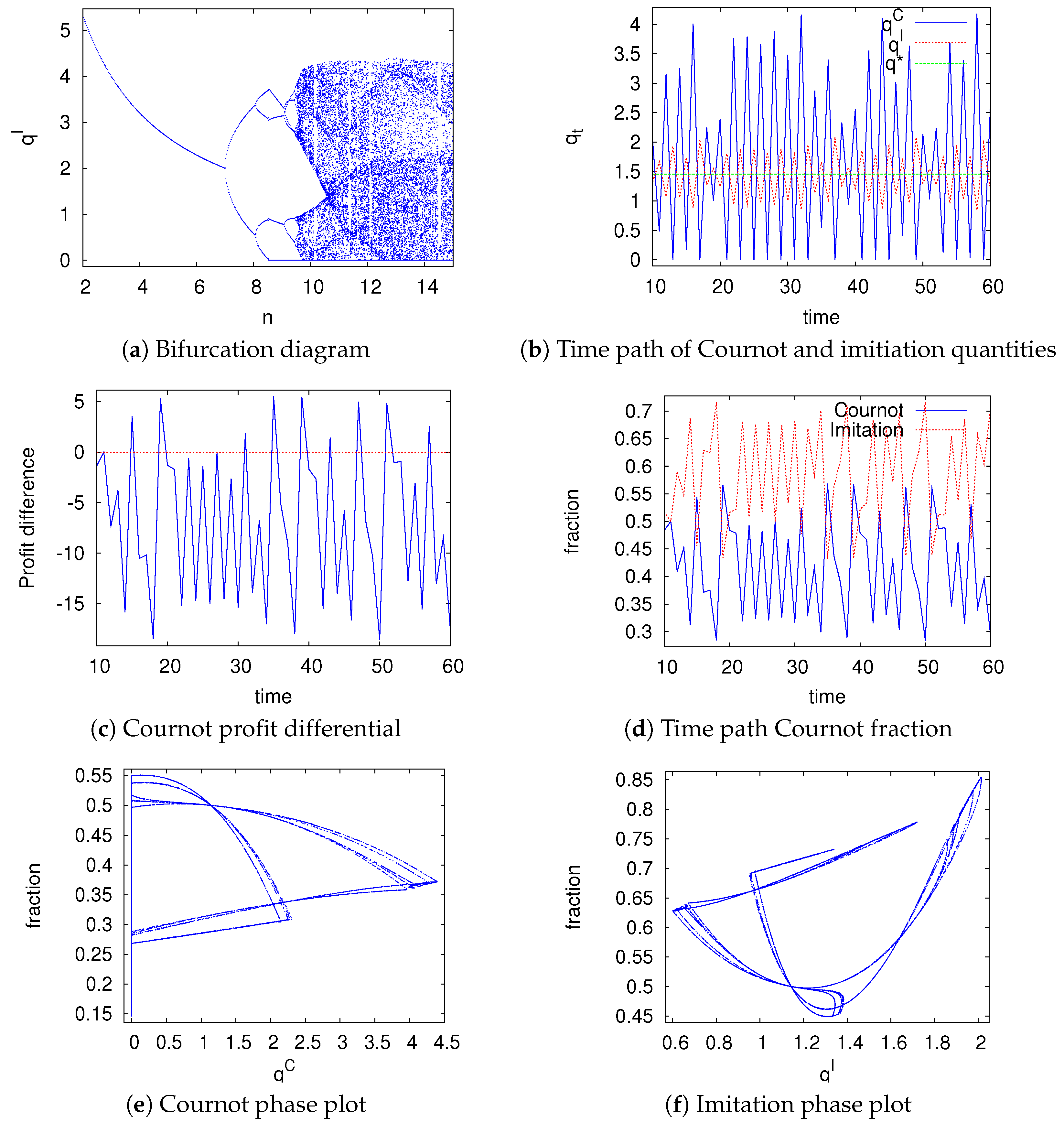
In Figure 1 the model is simulated under Logit-dynamics with intensity of choice parameter $\beta$, as in [26]. Panel (a) depicts a period-doubling route to chaotic quantity dynamics as the number of firms n increases. The first period-doubling bifurcation is for $n=7$ as calculated analytically. Panel (b) displays oscillating time series of produced quantity by the Cournot and imitation firms and the equilibrium quantity fraction $q^{*}$. As one can see the Cournot quantities are fluctuating more than the imitation quantities. The stabilizing effect of the imitation firms is here clearly visible, when Cournot firms produce more (less) then the Cournot-Nash equilibrium quantity, the imitation firms produce less (more) than the Cournot-Nash equilibrium quantity and therefore decrease the aggregated deviation from the equilibrium. Panel (c) displays the resulting Cournot profit differential ${\mathrm{\Pi }}^C-{\mathrm{\Pi }}^I$. Panel (d) displays the resulting oscillating time series of the Cournot and imitation fractions. In Panel (e) a phase portrait is shown for the Cournot heuristic whereas in Panel (f) a phase portrait for the imitation heuristic is shown. In Panel (g) the largest Lyapunov exponent for an increasing number of firms is shown. Game and behavioural parameters are equal set to: $n=10$, $a=17$, $b=1$, $c=1$, $C^C=0$, $C^I=0$, $\beta =0.05$. Initial conditions are set equal to: $q_0^C=0.8$, $q_0^I=0.8$, ${\eta }_0=0.5.$ When the evolutionary pressure increases, the system evolves to an equilibrium different from the Cournot-Nash equilibrium where the imitation firms produce more than the Cournot-Nash equilibrium whereas the Cournot firms produce less. Imitation profits are therefore much higher and as a consequence the complete population switches to the imitation heuristic.

The bifurcation diagram is re-plotted in Figure 2 under the same game and behavioral parameters and initial conditions, the only difference is that now $\beta =3$. When $1.7<n<2.8$ the imitation firms produce more then the Cournot-Nash equilibrium quantity while the Cournot firms produce less. This results in higher profits for the imitators and therefore the complete populations switches to imitators $(\eta =0)$. When $2.8\le n\le 3.2$ all firms produce the Cournot-Nash equilibrium quantity again, therefore profits and thus fractions are equal. When $n>3.2,$ the imitation firms produce again more then the equilibrium quantity while the Cournot firms produce less, except when n is close to $3.65$, then all firms produce the Cournot-Nash equilibrium quantity. Finally, when $n>5.6$ the imitation firms produce so much that the Cournot firms decide to produce nothing $(q^C=0)$.

4.2. Rational vs. Imitation Firms with Switching

As in the previous section, we need a 3-dimensional system to describe the dynamics of the model. The rational firms produce each period such that their expected profit is maximized whereas an imitator produces in the next period the currently average played quantity.

The rational quantity dynamics therefore have the following structure

$$q_t^R=\underset{q_i}{Argmax}E[P(q_{i,t}+Q_{-i,t})q_i-C\left(q_{i,t}\right)].$$

It forms expectations over all possible mixtures of heuristics resulting from randomly drawing $n-1$ other players from a large population, of which each with chance ${\eta }_t$ is a rational firm too, and with chance $1-{\eta }_t$ is a imitator. Rational firm i therefore chooses quantity $q_i$ such that his objective function, its own expected utility

$$U_t^R\left(q_{i,t}\right|q_t^R,q_t^I,{\eta }_t)={\sum }_{k=0}^{n-1}\left(\genfrac{}{}{0.0pt}{}{n-1}{k}\right){\eta }_t^k{(1-{\eta }_t)}^{n-1-k}[P((n-1-k)q_t^I+k{q}_t^R+q_{t,i})q_{t,i}-C\left(q_{t,i}\right)],$$

(22)

is maximized given the production of the other players and the population fraction. Here $q_t^R$ is the symmetric output level of each of the other rational firms in period t, and $q_t^I$ is the output level of each of the imitator firms in period t. The first order condition for an optimum is characterized by equality between marginal cost an expected marginal revenue.

Given the value of $q_t^I$ and the fraction ${\eta }_t$, all rational firms coordinate on the same output level $q_t^R$. This gives the first order condition

$$\frac{\delta U_t^R\left(q_{i,t}\right|q_t^R,q_t^I,{\eta }_t)}{\delta q_{i,t}}=0,$$

which equals to

$$\begin{array}{c}\sum _{k=0}^{n-1}\left(\genfrac{}{}{0.0pt}{}{n-1}{k}\right){\eta }_t^k{(1-{\eta }_t)}^{n-1-k}\times \\ \left[P\right((n-1-k)q_t^I+(k+1)q_t^R)+q_t^R{P}^{\prime }((n-1-k)q_t^I+(k+1)q_t^R)-C^{\prime }\left(q_t^R\right)]=0.\end{array}$$

(23)

Let the solution to Equation (23) be given by $q_t^R=H^R(q_t^I,{\eta }_t)$, the full system of equations is thus given by

$$\begin{array}{cc}\hfill q_{t+1}^R& =H^R(q_{t+1}^I,{\eta }_{t+1})\hfill \\ \hfill q_{t+1}^I& ={\eta }_t{q}_t^R+(1-{\eta }_t)q_t^I\hfill \\ \hfill {\eta }_{t+1}& =K(\Delta U_t).\hfill \end{array}$$

(24)

where $\Delta U_t=U_t^R-U_t^I$. It is easily checked that if the imitators play the Cournot-Nash equilibrium quantity $q^{*}$, or if all firms are rational, then the rational firms will play the Cournot-Nash equilibrium quantity, that is $H^R(q^{*},\eta )=q^{*}$, for all $\eta$ and $H^R(q^I,1)=q^{*}$ for all $q^I$. Moreover, if a rational firm is certain it will only meet imitation firms (that is $\eta =0$), it plays a best response to the currently average played quantity, that is $H^R(q_t^I,0)=R\left((n-1)q_t^I\right)$, for all $q_t^I$. In the remainder we will denote the partial derivatives of $H^R(q,\eta )$ with respect to q and $\eta$ by $H_q^R(q,\eta )$ and $H_{\eta }^R(q,\eta )$ respectively.

Proposition 4.

The Cournot-Nash equilibrium $(q^{*},q^{*})$ is a locally stable fixed point for the model with endogenous fractions of rational and imitation firms, where all firms produce the Cournot-Nash quantity, if and only if

$$|{\eta }^{*}{H}_q(q^{*},{\eta }^{*})+1-{\eta }^{*}|\hspace{0.17em}<1.$$

(25)

Proof. 

See Appendix A. □

Leading example. Since the stability condition is the similar to the condition derived in Section 3.2, the equilibrium quantities $(q^{*},q^{*})$ and rational play fraction ${\eta }^{*}$ is stable for all n in this linear specification.

5. Rational vs. Cournot vs. Imitation with Switching Heuristics

In this section we combine the ideas that we gathered in Section 4. We will investigate the dynamics when the three heuristics discussed before compete. As before every round n firms are drawn from a large pool of firms to play the one-shot Cournot game. From this large pool of firms a fraction ${\eta }_t^R$ plays according to the rational strategy in period t, a fraction ${\eta }_t^C$ plays according to the Cournot heuristic in period t and consequently the fraction of imitators in period t is determined by $1-{\eta }_t^R-{\eta }_t^C$. As in Section 4 the fitness of a heuristic is determined by the average payoff minus the information cost of using that heuristic. Again the average profits will be approximated by the expected profits but in contrast to Section 4 the distribution of states now follows a multinomial distribution instead of a binomial distribution. In general the average profit of a firm producing $q_1$ and competing with other firms that produce either $q_2$ or $q_3$ given the fractions ${\eta }_1$ and ${\eta }_2$ is stated below, in this average profit approximation the profit in each state is weighted by the chance of this state.

$$\begin{array}{c}{\mathrm{\Pi }}_{1,t}=F(q_{1,t},q_{2,t},q_{3,t},{\eta }_{1,t},{\eta }_{2,t})=\\ {\displaystyle \sum _{\Delta }\frac{(n-1)!}{k_1!k_2!(n-k_1-k_2-1)!}{\eta }_{1,t}^{k_1}{\eta }_{2,t}^{k_2}{(1-{\eta }_{1,t}-{\eta }_{2,t})}^{n-k_1-k_2-1}\times }\\ P((k_1+1)q_{1,t}+k_2{q}_{2,t}+(n-1-k_1-k_2)q_{3,t})q_{1,t}-C\left(q_{1,t}\right).\end{array}$$

(26)

The summation is over all possible combinations of $k_1$ and $k_2$, which stand for the number of other firms producing $q_1$ and $q_2$ respectively, that is: $\Delta =\{k_1,k_2\in {\mathbb{I}}^2:0\le k_1\le n-1;0\le k_2\le n-1;0\le k_1+k_2\le n-1\}.$ Expected profits for heuristic 2 in period t are given by $F(q_{2,t},q_{1,t},q_{3,t},{\eta }_{2,t},{\eta }_{1,t})$, expected profits for heuristic 3 in period t are given by $F(q_{3,t},q_{2,t},q_{1,t},1-{\eta }_{1,t}-{\eta }_{2,t},{\eta }_{2,t})$.

The complete dynamical system consists of five equations, three for the quantity dynamics and two to describe how the fractions evolve. As in all previous sections, the Cournot firms play in the next period a best-response to the current aggregated output of the others, imitators play in the next period the average produced quantity by the others in the current period. Rational players produce every period the quantity that maximizes expected payoff given the fractions and production plans of all other firms (imitators, Cournot players but rational players too). The rational firms produce expectations over all possible mixtures of heuristics resulting from randomly drawing the $n-1$ other players from the large population of firms. In this setting the rational objective function, its own expected utility is of the following form:

$$\begin{array}{cc}\hfill U_t^R\left(q_{i,t}\right|\mathbf{x})=& {\displaystyle \sum _{\Delta }{f}_{k_1,k_2}(n-1,{\eta }^R,{\eta }^C)\times }\hfill \\ \hfill & P(k_1{q}_t^R+k_2{q}_t^C+(n-1-k_1-k_2)q_t^I+q_{i,t})q_{i,t}-C\left(q_{i,t}\right),\hfill \end{array}$$

(27)

with $f_{k_1,k_2}(n-1,{\eta }^R,{\eta }^C)=\frac{(n-1)!}{k_1!k_2!(n-k_1-k_2-1)!}{{\eta }_t^R}^{k_1}{{\eta }_t^C}^{k_2}{(1-{\eta }_t^R-{\eta }_t^C)}^{n-k_1-k_2-1}$ denotes the multinomial distribution of three heuristics in the population of firms and $\mathbf{x}=(q_t^R,q_t^I,q_t^C,{\eta }_t^R,{\eta }_t^C)$ the system’s state variables. The first order condition for an optimum of (27) is characterized by equality between marginal cost an expected marginal revenue.

Given the value of $q_t^C$$q_t^I$${\eta }_t^R$${\eta }_t^C$, all rational firms coordinate on the same output level $q_t^R$. Differentiating Equation (27) with respect to $q_{i,t}$ gives the first order condition, which is equal for all rational firms. This first order condition is given by:

$$\frac{\delta U_t^R\left(q_{i,t}\right|\mathbf{x})}{\delta q_{i,t}}=0$$

which equals to:

$$\begin{array}{c}{\displaystyle \sum _{\Delta }{f}_{k_1,k_2}(n-1,{\eta }^R,{\eta }^C)\times }\\ \left[P\right((k_1+1)q_t^R+k_2{q}_t^C+(n-1-k_1-k_2)q_t^I)+\\ P^{\prime }((k_1+1)q_t^R+k_2{q}_t^C+(n-1-k_1-k_2)q_t^I)q_t^R-C^{\prime }\left(q_t^R\right)]=0.\end{array}$$

(28)

Let the solution to this be given by $q_t^R=H^R(q_t^C,q_t^I,{\eta }_t^R,{\eta }_t^C)$. The system of quantity dynamics is thus given by

$$\begin{array}{cc}\hfill q_{t+1}^R& =H^R(q_{t+1}^C,q_{t+1}^I,{\eta }_{t+1}^R,{\eta }_{t+1}^C)\hfill \\ \hfill q_{t+1}^C& =R((n-1)({\eta }_t^R{q}_t^R+{\eta }_t^C{q}_t^C+(1-{\eta }_t^R-{\eta }_t^C)q_t^I)\hfill \\ \hfill q_{t+1}^I& ={\eta }_t^R{q}_t^R+{\eta }_t^C{q}_t^C+(1-{\eta }_t^R-{\eta }_t^C)q_t^I\hfill \end{array}$$

(29)

Note that rational player plays such that expected marginal revenue equals marginal cost at $t+1$ and a Cournot firm plays such that its marginal revenue (of period t) equals marginal cost (at period t). Therefore the Cournot heuristic is a lagged version of the rational heuristic if and only if

$$\begin{array}{c}{P}^{\prime R}{q}^R+{\eta }^C{q}^C+(1-{\eta }^R-{\eta }^C)q^I)+q^C)=\\ {\displaystyle \sum _{\Delta }{f}_{k_1,k_2}(n-1,{\eta }^R,{\eta }^C)P^{\prime }((k_1+1)q^R+k_2{q}^C+(n-1-k_1-k_2)q^I).}\end{array}$$

(30)

Thus the Cournot heuristic is only a lagged version of the rational heuristic if the inverse demand is linear. In this specific case the analysis become easier because this gives the possibility to lower the dimension of the dynamical system.

It is easily checked that if the imitation and Cournot firms play the Cournot-Nash equilibrium quantity $q^{*}$, or if all firms are rational, the rational firms will play the Cournot-Nash equilibrium quantity, that is $H^R(q^{*},q^{*},{\eta }_t^R,{\eta }_t^C)=q^{*}$, for all ${\eta }^R$ and ${\eta }^C$ and $H^R(q_{t+1}^C,q_{t+1}^I,1,0)=q^{*}$ for all $q^C$, $q^I$. In the remainder we will denote by $H_{q^R}^R$, $H_{q^C}^R$, $H_{q^I}^R$, $H_{{\eta }^R}^R$ and $H_{{\eta }^C}^R$ the partial derivatives of $H^R(q^C,q^I,{\eta }^R,{\eta }^C)$ with respect to $q^R$, $q^C$, $q^I$, ${\eta }^R$ and ${\eta }^C$ respectively, evaluated at the equilibrium $(q^{*},q^{*},q^{*},{\eta }^{R^{*}}{\eta }^{C^{*}})$, which we will denote by $x^{*}$ in the remainder of this chapter for notational convenience.

Now that we have the quantity dynamics we can turn to the population dynamics. These are related to the population dynamics from Section 4 but differ significantly since we are in a three heuristic environment now. The population dynamics, as in Section 4, depend on relative fitness. Let the fraction dynamics be given by

$$\begin{array}{cc}\hfill {\eta }_{R,t+1}& =K^R(\Delta U_t^R,\Delta U_t^C)\hfill \\ \hfill {\eta }_{C,t+1}& =K^C(\Delta U_t^R,\Delta U_t^C),\hfill \end{array}$$

(31)

where ${\eta }_{t+1}^R$ is the fraction of rational firms in period $t+1$ whereas ${\eta }_{t+1}^C$ is the fraction of Cournot firms in that period. Denoting the rational, Cournot and imitation heuristics’ costs by $C^R,$ $C^C,C^I,$ respectively, we obtain $\Delta U_t^R=({\mathrm{\Pi }}_t^R-C^R)-({\mathrm{\Pi }}_t^C-C^C)$, the difference in average fitness of the rational and the Cournot heuristic, and, $\Delta U_t^C=({\mathrm{\Pi }}_t^C-C^C)-({\mathrm{\Pi }}_t^I-C^I)$ the difference in average fitness of the Cournot and the imitation heuristic. Note that $K^R$ and $K^C$ are ${\mathbb{R}}^2\to [0,1]$ are continuously differentiable functions where the difference in fitness of the rational and Cournot heuristics and the difference in fitness of the Cournot and imitation heuristic are used as input. The difference in fitness of the rational and imitation heuristic is not used as an input variable since this information is captured implicitly in the other two differences. Note that $K^R$ is a monotonically increasing function in the first and second element whereas $K^C$ is decreasing in the first element but increasing in the second element. Furthermore, $K^R(0,0)=K^C(0,0)=\frac{1}{3}$. In the remainder of this chapter we denote $K_1^R$ and $K_2^R$ the partial derivatives of $K^R$ with respect to the first and the second element respectively and with $K_1^C$ and $K_2^C$ the partial derivatives of $K^C$ with respect to the first and the second element respectively.

The full system of quantity and population dynamics is given by:

$$\begin{array}{cc}\hfill q_{t+1}^R={\varphi }^1& =H^R({\varphi }^2,{\varphi }^3,{\varphi }^4,{\varphi }^5)\hfill \\ \hfill q_{t+1}^C={\varphi }^2& =R((n-1)({\eta }_t^R{H}^R(q_t^C,q_t^I,{\eta }_t^R,{\eta }_t^C)+{\eta }_t^C{q}_t^C+(1-{\eta }_t^R-{\eta }_t^C)q_t^I)\hfill \\ \hfill q_{t+1}^I={\varphi }^3& ={\eta }_t^R{q}_t^R+{\eta }_t^C{q}_t^C+(1-{\eta }_t^R-{\eta }_t^C)q_t^I\hfill \\ \hfill {\eta }_{t+1}^R={\varphi }^4& =K^R(\Delta U_t^R,\Delta U_t^C)\hfill \\ \hfill {\eta }_{t+1}^C={\varphi }^5& =K^C(\Delta U_t^R,\Delta U_t^C).\hfill \end{array}$$

(32)

Since a dynamical system can only depend on lagged variables we substituted ${\varphi }^2,{\varphi }^3,{\varphi }^4,{\varphi }^5$ into $H^R(·)$. In order to determine the local stability of the unique, interior equilibrium ${\mathbf{x}}^{*},$ we need to determine the eigenvalues of the Jacobian matrix evaluated at that equilibrium. The Jacobian of the general oligopoly-general selection dynamic $K(·)$ has very complicated eigenvalues which cannot be expressed in useful functions (see Appendix A, Proof of Proposition 5, for the full Jacobi matrix), therefore we will restrain the subsequent analysis to the linear-demand, linear-cost oligopoly with Logit Dynamics.

Leading example. We know that the Cournot heuristic is a lagged version of the rational heuristic in this leading example since the inverse demand function is linear, therefore the dimension of the dynamical system can be reduced by one. Note that only the Cournot production is a lagged version of the rational production. The Cournot profits and resulting fractions are in general not lagged rational profits and fractions. Therefore, the restriction of the complete, 5-dim dynamical system to the linear-linear oligopoly with Logit Dynamics becomes 4-dim

$$\begin{array}{cc}\hfill q_{t+1}^C& ={\varphi }^1\left({\mathbf{x}}_t\right)=\frac{1}{2+{\eta }^R(n-1)}\left(\frac{a-c}{2b}-\frac{1}{2}(n-1)({\eta }_t^C{q}_t^C+(1-{\eta }^R-{\eta }^C)q_t^I)\right)\hfill \\ \hfill q_{t+1}^I& ={\varphi }^2\left({\mathbf{x}}_t\right)={\eta }_t^R{\varphi }^1\left(x\right)+{\eta }_t^C{q}_t^C+(1-{\eta }^R-{\eta }^C)q_t^I\hfill \\ \hfill {\eta }_{t+1}^R& ={\varphi }^3\left({\mathbf{x}}_t\right)=\frac{e^{\beta \Delta U_t^R}}{e^{\beta \Delta U_t^R}+1+e^{-\beta \Delta U_t^C}}\hfill \\ \hfill {\eta }_{t+1}^C& ={\varphi }^4\left({\mathbf{x}}_t\right)=\frac{e^{\beta \Delta U_t^C}}{e^{\beta (\Delta U_t^R+\Delta U_t^C)}+e^{\beta \Delta U_t^C}+1}.\hfill \end{array}$$

(33)

This system has one unique equilibrium where all firms produces the Cournot-Nash quantity $q^{*}$. Since production is equal at the equilibrium, profits are equal at the equilibrium. The equilibrium fractions are therefore a function of the information costs and the evolutionary pressure, given by

$${{\eta }^R}^{*}=\frac{e^{\beta (C^C-C^R)}}{e^{\beta (C^C-C^R)}+1+e^{-\beta (C^I-C^C)}}\mathrm{and}{{\eta }^C}^{*}=\frac{e^{\beta (C^I-C^C)}}{e^{\beta (C^I-C^R)}+e^{-\beta (C^I-C^C)}+1}.$$

For general heuristics’ costs—and, therefore, general fractions ${{\eta }^R}^{*}$ and ${{\eta }^C}^{*}$—the eigenvalues of the corresponding Jacobian at the rest point are convoluted expressions of model’s parameters, which cannot be meaningfully simplified. Nevertheless, because the rational heuristic is more informationally- and computationally-intensive than the Cournot and the imitation heuristics, it is reasonable to assume a strictly positive cost $C^R>0$ associated to its use, while setting the costs of the other two heuristics $C^C=C^I=0$. We obtain the following result:

Proposition 5.

For costly, rational heuristic $(C^R>0)$ and, costless, Cournot and imitation heuristics $(C^C=C^I=0),$ the interior, Cournot-Nash equilibrium $(q^{*},q^{*},q^{*})$ along with equilibrium fractions ${\eta }^{R*}=\frac{e^{-\beta C^R}}{e^{-\beta C^R}+2}$$,{{\eta }^C}^{*}={{\eta }^I}^{*}=\frac{1}{e^{-\beta C^R}+2},$ is a locally stable fixed point for the model with endogenous fluctuations between of rational, Cournot and imitation firms, if and only if

$$n<\psi \left({C^R}^{*}\beta \right)=\frac{7e^{C^R\beta }+1}{e^{C^R\beta }-1}.$$

(34)

From Equation (34) we notice first that, when information cost of the rational play $C^R$ approaches zero, the system is stable for all market sizes $n.$ If the cost differential of rational vs. Cournot and imitation play is strictly positive $(C^R>0)$ and intensity of selection $\beta \to \infty ,$ the equilibrium is stable for $n<7.$ For, intermediate, finite $\beta$, the equilibrium fractions $({\eta }^{R*},{{\eta }^C}^{*},{{\eta }^I}^{*})$, as well as the instability threshold n are a function of both $C^R$ and $\beta .$ In the simulations below, $C^R=1$ and $\beta =3$, the equilibrium $\left(\frac{a-c}{b(n+1)},\frac{a-c}{b(n+1)},\frac{e^{-3}}{e^{-3}+2},\frac{1}{e^{-3}+2}\right)$ is stable when $n<7.42$. When $n=7.42$, the system undergoes its first bifurcation. The largest eigenvalue is equal to $-1$ at the bifurcation, indicating that the first bifurcation is a period-doubling bifurcation. This is confirmed by the simulations below.

The leading example is simulated in Figure 3. Panel (a) depicts the bifurcation diagram for increasing number of firms n. The first period-doubling bifurcation appears, as calculated analytically for $n=7.42$. For $n=11.85$, the system undergoes a Hopf-bifurcation which creates highly non-linear dynamics. For $13\le n\le 14.4$, the system is in a 10-cycle whereas for $n>14.4$ the system becomes chaotic again. Panel (b) displays oscillating time series of produced quantity by the Cournot and imitation firms and the equilibrium quantity fraction $q^{*}$. Since the rational quantity in period $t+1$ equals the Cournot quantity in period t this time series is not included. Panel (c) displays the resulting profits. Note that ${\mathrm{\Pi }}_t^I>{\mathrm{\Pi }}_t^R\forall t$ and ${\mathrm{\Pi }}_t^I\ge {\mathrm{\Pi }}_t^C\forall t$. Panel (d) displays the resulting oscillating time series of the fraction fractions. Due to the information cost the sophisticated rational firms do not perform better than the Cournot and imitation firms resulting in low fractions of rational firms. Moreover, since the imitation profit is at least as high as the Cournot profit, the resulting imitation fraction is at least as high as the Cournot fraction. In Panel (e) the largest Lyapunov exponent for increasing number of firms is shown whereas in Panel (f) the largest Lyapunov exponent for increasing $\beta$ is shown. Game and behavioural parameters are set equal to: $n=19$, $a=17$, $b=1$, $c=1$, $C^R=1$, $C^C=0$, $C^I=0$, $\beta =3$. Initial conditions are set equal to: $q_0^R=0.3$, $q_0^C=0.1$, $q_0^I=0.25$, ${\eta }_0^R=0.5$, ${\eta }_0^C=0.2$.

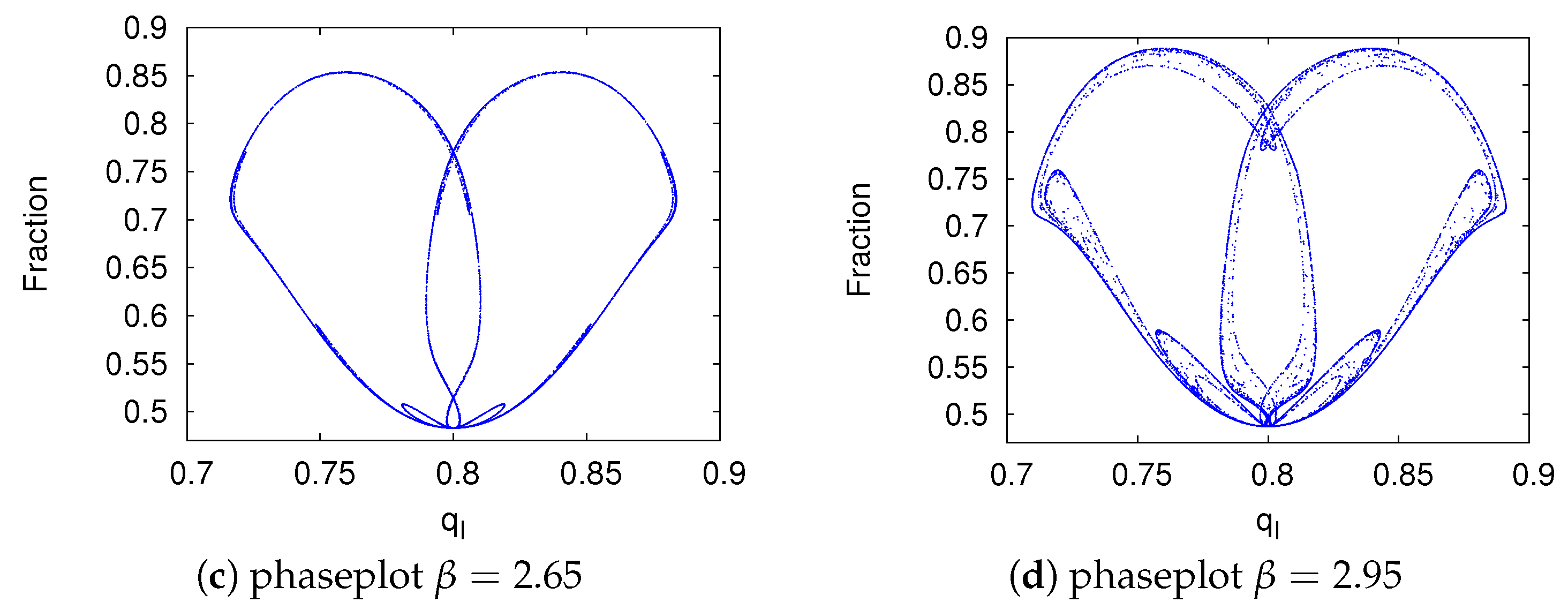
Last, Figure 4 shows some attractors of the evolutionary model for increasing evolutionary pressure, with (quasi-)periodic motion just after the second bifurcation and breaking of the invariant circles into a strange attractor as the number of firms further increases. Similar ‘breaking of the invariant circles’ route to chaos appears for the rational and Cournot series.

6. Concluding Remarks

In this paper we set out to filling a gap in the literature on heterogenous heuristics in a Cournot oligopoly with boundedly rational players. Partly motivated by the experimental evidence for imitate-the-average behaviors in oligopoly games, our focus is on better understanding the role this specific imitation rule plays in a competitive Cournot environment, populated by myopic best-reply and rational (equilibrium) firms. In a population game framework- random re-matching of players, with fitness approximated by the expected payoffs accruing in all possible realizations of opponents’ heuristic types—the interplay between two model’s parameters—differential cost C between heuristics and intensity of evolutionary selection acting upon heuristics $\beta$-determines the critical market size for which the unique, interior Cournot-Nash equilibrium of the underlying oligopoly loses stability.

For the pairwise, evolutionary contests between heuristics we first showed that in the case when Cournot firms compete with imitators, if $C>0$ (imitation heuristic enjoys a strict cost advantage over the myopic Cournot adjustment) and intensity of selection $\beta$ is very large ($\beta \to \infty$ limit), then the Cournot equilibrium is locally stable for $n<7.$ Absent the information costs’ differential (i.e., $C=C_C-C_I=0),$ the threshold on the number of firms that changes the system from stable to unstable remains 7, irrespective of the magnitude of the evolutionary pressure $\beta .$ In contrast with the model comprising Cournot players only (Cournot equilibrium already unstable for $n=3)$, the addition of players using the relatively cheaper imitate-the-average heuristic, stabilizes the equilibrium. Secondly, in the situation when rational firms compete with imitators, the system is always stable, regardless of the information costs of the more sophisticated, rational choice.

For the full ecology of behavioral rules—rational firms, Cournot firms and imitators—we are able to derive the (in)stability threshold on the number of firms for the linear inverse demand-linear costs oligopoly with Logit Dynamics and for a particular configuration of heuristics costs: costly rational heuristic $(C^R\ge 0)$ and costless Cournot and imitation rules $(C^C=C^I$$=0)$. On one hand, if rational plays is costless, the equilibrium is stable, for all possible market sizes $n$. On the other hand, even for small, strictly positive $C^R,$ the interior, Cournot equilibrium loses stability for $n=7$ (in the $\beta \to \infty$ limit) and for larger market sizes $n>7$ (in the case of finite $\beta$). Complicated endogenous fluctuations (two-cycles, strange attractors) in the quantities played and the fractions of various heuristics may occur, in particular, when the evolutionary pressure is high.

By deriving the stability conditions for our pairwise and threewise evolutionary model, we conclude that introducing imitators tends to stabilize the dynamics, provided that imitation is the least costly heuristics in the menu of potential learning rules.

At least two avenues seem promising for future research: firstly, our analysis deals with Cournot oligopolies that display an unique, interior Cournot-Nash equilibrium, and, therefore, we conjecture that our local stability analysis also holds globally. This is, of course, not valid for the Type II oligopolies that display multiple—interior and boundary—Nash equilibria. How the (in)stability of these equilibria, along with the relative size of their basins of attraction, vary with the market size n, under the full ecology of three, switching heuristics proposed in this paper, remains an unexplored question.

Secondly, related to the implications of imitative behavior in heterogenous heuristics environments, it would be worth considering alternative models of imitation. Our way of modelling imitation favors the average play (imitate the average behavior in the population) but other imitation rules well-studied in the literature may be envisaged. For instance, a version of the imitation heuristic that copies the past production decision of the most profitable firm from the entire population or one that imitates the successful players only among the m closest neighbors (in a location model, à la Hotelling). In these alternative imitation scenarios, coordination on a non-Cournot equilibrium—for instance, on the Walrasian equilibrium as in [8] under the homogeneous, imitate-the-best play—may arise.

References

- Theocharis, R.D. On the stability of the Cournot solution on the oligopoly problem. Rev. Econ. Stud. 1960, 27, 133–134. [Google Scholar] [CrossRef]
- Cournot, A. Researches into the Mathematical Principles of the Theory of Wealth; Bacon, N.T., Translator; Macmillan Co.: New York, NY, USA, 1897. [Google Scholar]
- Droste, E.; Hommes, C.; Tuinstra, J. Endogenous fluctuations under evolutionary pressure in Cournot competition. Games Econ. Behav. 2002, 40, 232–269. [Google Scholar] [CrossRef]
- Hommes, C.; Ochea, M.; Tuinstra, J. Evolutionary Competition between Adjustment Processes in Cournot Oligopoly: Instability and Complex Dynamics. Dyn. Games Appl. 2018, 8, 822–843. [Google Scholar] [CrossRef]
- Huck, S.; Normann, H.T.; Oechssler, J. Stability of the Cournot process experimental evidence. Int. J. Game Theory 2002, 31, 123–136. [Google Scholar] [CrossRef]
- Cox, J.C.; Walker, M. Learning to play Cournot duopoly strategies. J. Econ. Behav. Organ. 1998, 36, 141–161. [Google Scholar] [CrossRef]
- Moreno, D.; Walker, M. Two problems in applying Ljung’s ‘projection algorithms’ to the analysis of decentralized learning. J. Econ. Theory 1994, 62, 420–427. [Google Scholar] [CrossRef]
- Vega-Redondo, F. The evolution of Walrasian behavior. Econometrica 1997, 65, 275–284. [Google Scholar] [CrossRef]
- Bosch-Domenech, A.; Vriend, N. Imitation of succesful behaviour in cournot markets. Econ. J. 2003, 113, 495–524. [Google Scholar]
- Schipper, B. Imitators and optimizers in Cournot oligopoly. J. Econ. Dyn. Control 2009, 33, 1981–1990. [Google Scholar] [CrossRef]
- Duersch, P.; Oechssler, J.; Schipper, B.C. Unbeatable imitation. Games Econ. Behav. 2012, 76, 88–96. [Google Scholar] [CrossRef]
- Duersch, P.; Oechssler, J.; Schipper, B.C. When is tit-for-tat unbeatable? Int. J. Game Theory 2014, 43, 25–36. [Google Scholar] [CrossRef]
- Duersch, P.; Kolb, A.; Oechssler, J.; Schipper, B. Rage Against the Machines: How Subjects Learn to Play Against Computers. Econ. Theory 2010, 43, 407–430. [Google Scholar] [CrossRef]
- Kaniovski, Y.; Kryazhimskii, A.V.; Young, H.P. Adaptive Dynamics in Games Played by Heterogeneous Populations. Games Econ. Behav. 2000, 31, 50–96. [Google Scholar] [CrossRef]
- Juang, W.-T. Rule Evolution and Equilibrium Selection. Games Econ. Behav. 2002, 39, 71–90. [Google Scholar] [CrossRef]
- Josephson, J. Stochastic adaptation in finite games played by heterogeneous populations. J. Econ. Dyn. Control 2009, 33, 1543–1554. [Google Scholar] [CrossRef]
- Khan, A. Evolutionary stability of behavioural rules in bargaining. J. Econ. Behav. Organ. 2021, 187, 399–414. [Google Scholar] [CrossRef]
- Maynard Smith, J.; Price, J. The logic of animal conflict. Nature 1973, 246, 15–18. [Google Scholar] [CrossRef]
- Frank, R. If Homo Economicus Could Choose His Own Utility Function, Would He Want One with a Conscience? Am. Econ. Rev. 1987, 77, 593–604. [Google Scholar]
- Güth, W.; Yaari, M. An Evolutionary Approach to Explaining Reciprocal Behavior in a Simple Strategic Game. In Explaining Process and Change; Witt, U., Ed.; The University of Michigan Press: Ann Arbor, MI, USA, 1992. [Google Scholar]
- Dekel, E.; Ely, J.C.; Yilankaya, O. Evolution of Preferences. Rev. Econ. Stud. 2007, 74, 685–704. [Google Scholar] [CrossRef]
- Fershtman, C.; Judd, K.L. Equilibrium Incentives in Oligopoly. Am. Econ. Rev. 1987, 77, 927–940. [Google Scholar]
- Kopel, M.; Lamantia, F.; Szidarovszky, F. Evolutionary competition in a mixed market with socially concerned firms. J. Econ. Dyn. Control 2014, 48, 394–409. [Google Scholar] [CrossRef]
- Szidarovszky, F.; Yakowitz, S. A new proof of the existence and uniqueness of the Cournot equilibrium. Int. Econ. Rev. 1977, 18, 783–789. [Google Scholar] [CrossRef]
- Wiggins, S. Introduction to Applied Nonlinear Dynamical Systems and Chaos; Springer: New York, NY, USA, 2003. [Google Scholar]
- Brock, W.; Hommes, C.H. A rational route to randomness. Econometrica 1997, 65, 1059–1095. [Google Scholar] [CrossRef]
- Tuinstra, J. Price Dynamics in Equilibrium Models. Ph.D. Thesis, Tinbergen Institute, Amsterdam, The Netherlands, 1999. [Google Scholar]
Figure 1.
Linear n-player Cournot game with endogenous fraction dynamics.
Figure 2.
Bifurcation diagram with .
Figure 3.
Linear n-player Cournot competition between rational, Cournot and imitation firms with endogenous fraction dynamics.
Figure 4.
Phaseplots (qI, ηI), for increasing evolutionary pressure.
Disclaimer/Publisher’s Note: The statements, opinions and data contained in all publications are solely those of the individual author(s) and contributor(s) and not of MDPI and/or the editor(s). MDPI and/or the editor(s) disclaim responsibility for any injury to people or property resulting from any ideas, methods, instructions or products referred to in the content. |
© 2024 by the authors. Licensee MDPI, Basel, Switzerland. This article is an open access article distributed under the terms and conditions of the Creative Commons Attribution (CC BY) license (https://creativecommons.org/licenses/by/4.0/).
Share and Cite
MDPI and ACS Style
Lindeman, D.; Ochea, M.I. Imitation Dynamics in Oligopoly Games with Heterogeneous Players. Games 2024, 15, 8. https://0-doi-org.brum.beds.ac.uk/10.3390/g15020008
AMA Style
Lindeman D, Ochea MI. Imitation Dynamics in Oligopoly Games with Heterogeneous Players. Games. 2024; 15(2):8. https://0-doi-org.brum.beds.ac.uk/10.3390/g15020008
Chicago/Turabian StyleLindeman, Daan, and Marius I. Ochea. 2024. "Imitation Dynamics in Oligopoly Games with Heterogeneous Players" Games 15, no. 2: 8. https://0-doi-org.brum.beds.ac.uk/10.3390/g15020008
Note that from the first issue of 2016, this journal uses article numbers instead of page numbers. See further details here.