Closed-Form Formulation of the Thermodynamically Consistent Electrochemical Model Considering Electrochemical Co-Oxidation of CO and H₂ for Simulating Solid Oxide Fuel Cells

Abstract

Achieving efficient solid oxide fuel cell operation and simultaneous prevention of degradation effects calls for the development of precise on-line monitoring and control tools based on predictive, computationally fast models. The originality of the proposed modelling approach originates from the hypothesis that the innovative derivation procedure enables the development of a thermodynamically consistent multi-species electrochemical model that considers the electrochemical co-oxidation of carbon monoxide and hydrogen in a closed-form. The latter is achieved by coupling the equations for anodic reaction rates with the equation for anodic potential. Furthermore, the newly derived model is capable of accommodating the diffusive transport of gaseous species through the gas diffusion layer, yielding a computationally efficient quasi-one-dimensional model. This resolves a persistent knowledge gap, as the proposed modelling approach enables the modelling of multi-species fuels in a closed form, resulting in very high computational efficiency, and thus enable the model’s real-time capability. Multiple validation steps against polarisation curves with different fuel mixtures confirm the capability of the newly developed model to replicate experimental data. Furthermore, the presented results confirm the capability of the model to accurately simulate outside the calibrated variation space under different operating conditions and reformate mixtures. These functionalities position the proposed model as a beyond state-of-the-art tool for model supported development and control applications.

1. Introduction

Solid oxide fuel cells (SOFCs) are a promising and emerging technology with high efficiency and very versatile fuel flexibility. Besides their instrumental role in the envisaged uptake of a hydrogen economy, they are also one of the key components in future thermochemical conversion processes, which will also have a strong role in future energy systems. Either through gasification or combustion, thermochemical conversion processes are expected to represent an important supportive technology required to preserve energy supply stability and to enable the conversion of challenging energy carriers such as the steadily increasing anthropogenic waste. The latter is also addressed with gasification, resulting in synthesis gas, one of the most promising second-generation fuels. The composition of the synthesis gas produced is highly dependent on the type of waste biomass and on the gasification technology [1,2]. It can also be controlled by operational conditions [3,4] or altered using catalysts [5,6]. Even though the utilisation of synthesis gas in internal combustion engines offers relatively high efficiency [7], SOFCs provide several advantages over these traditional energy conversion systems, namely high efficiency, relatively low levels of emissions, and long-term stability and fuel flexibility. Exactly this aforementioned fuel flexibility, which can be achieved with an appropriate pre-treatment system with the aim of avoiding intensified degradation from carbon deposition, exposure to tar, hydrogen sulphide, hydrogen chloride, and alkali metals on the SOFC anode [8], enables the utilisation of various fuels ranging from synthesis gasses to hydrogen as well as multiple other fuels. In combination with very high conversion efficiency to electric energy, these properties characterise SOFCs as a very promising component of future energy systems.

The simultaneous reduction in production costs and the extension of service life while maintaining high system efficiency are considered major challenges in their wider market adoption. Reaching these objectives calls for the application of advanced virtual tools over the entire product lifecycle management. Therefore, this paper addresses a specific challenging aspect of developing an advanced system level model featuring physicochemical consistency with detailed mechanistic models. These advanced system level models ensure high accuracy while featuring sufficiently short computational times. Such models can be used in the left arm of the V-development process due to their mechanistic basis ensuring high accuracy and extrapolation capability. When such models also feature real-time capability, they can be applied in the right arm of the V-development process in control, digital twin, and hardware-in-the-loop (HiL) applications, where good extrapolation capabilities also significantly enhance the applicability and accuracy of the model, as it can be parametrised on smaller data sets. Fast running mechanistic models enable the introduction of new functionalities such as advanced State of X—SoX (e.g., state of operational conditions (SoOC), state of health (SoH), and State of Function (SoF)) observers, further pushing the boundaries of performance and service life optimisations as well as predictive maintenance and failure analysis.

Considering the listed objectives, the data-driven models of SOFC operation relying on, e.g., neural network modelling [9,10], or Hammerstein–Wiener models [11] that are commonly utilised in the system level analyses have limited applicability, since their accuracy does not reach, in general, beyond the calibration space of parameters. The latter proves to be especially cumbersome for FC applications due to the effects of the curse of dimensionality [12]. These deficiencies motivate the use of computationally fast Reduced Dimensionality Electrochemical Models (RDEM) featuring a more profound physicochemically consistent mechanistic basis, as for example derived in [13] for single fuel Proton-exchange membrane (PEM) fuel cells. Such types of models can be parametrised by experimental data or based on 3D Computational Fluid Dynamics (CFD) results or other models with higher fidelity. RDEMs possess better extrapolation capabilities for operational points outside the calibration space of the model, as they use a more consistent physicochemical basis, e.g., [13]. The literature offers multiple types of physicochemically inspired reduced dimensionality models considering a single fuel [13,14,15] that are derived in a closed-form, which is crucial to achieving very low computational efforts as well as HiL compliance.

However, the present system level models of SOFCs, for example [16,17,18,19,20,21,22,23,24,25,26] that are applied in performance [16,17,18,20,21,23,24,25] and service life [19,22] predictions, and optimisations do not feature both of these requirements, i.e., the derivation of activation losses and utilisation ratios for multiple fuel species in a closed-form, and physicochemical consistency. Models, such as [16,17,18,19,20,21,22,23,26], model from the electrochemical point of view of only a single reactant component fuel (hydrogen) and neglect the CO, and calculate its effects only via energy balances or via the water–gas shift reaction (WGSR) without addressing the kinetics of electrochemical co-oxidation. On the other end, these models aiming to address multi-component kinetics observed in SOFC are also being developed [24,25,27,28,29,30,31,32,33,34,35,36,37]; however, they are usually embedded in higher fidelity models [27,28,29,30,31,32,33,34,35,36,37], ranging from 1D+1D [25] over 2D [28,29,31,32,34,35,36,37] to 3D [29,30]. For a more in-depth review of these and other models, the reader is referred to the review article published by Bao et al. [38]. In References [24,25,39,40,41,42,43], the authors model multi-reactant fuel electrochemistry on the system level and are thus physicochemically consistent. However, the electrochemical models utilised in [24,25,39,40,41,43] obtain the overall voltage and over-potentials with a linearised Tafel equation or in an iterative manner, which inherently leads to increased computational times, preventing their use in SoX and HiL applications. In contrast, in [42,44], the approximate solution is obtained by decoupling the charge and mass transfer and by neglecting the effect of species concentration on electrochemical kinetics. This missing combination of physicochemically consistent treatment of multiple fuels in a closed-form model thus represents a clear knowledge gap that is tackled in this paper.

An additional knowledge gap in need of addressing in the area of reduced dimensionality performance models, where models are commonly modelled by the Butler–Volmer (BV) equation with the aim of achieving high prediction capability in the entire current range and thus the entire range of net reaction rates, is obtaining the inverse of the BV equation with the respect to the voltage. Some authors address this issue by utilising fully empirical models in [19], the Tafel equation in [16,29,31,45], a linearised Tafel equation [36,37,40,41], and a modified Tafel equation with the natural logarithm replacement with a sinus hyperbolicus [18,20,21,23,28]. The overall assumption needed for the derivation of electrochemical models based on the Tafel equation is that the the reaction from reactants to products overshadows the backwards reaction, i.e., the reaction from products to reactants. This assumption proves to be justified for high activation over-potentials and consequential high current densities or molar fluxes but has a significant deficiency in the region with low activation over-potentials, where the approximation error increases exponentially when current density or molar flux approaches zero, which inevitably means that the activation losses cannot be determined with sufficient accuracy.

To resolve this persisting knowledge gap and to present significant progress in the aforementioned area, this paper introduces an innovative framework of a computationally fast multi-species thermodynamically consistent RDEM of SOFC with co-oxidation of CO and H${}_2$ based on the closed-form solution using the BV equation. The latter is derived from the anodic and cathodic reaction rates over the BV equation to the final form using a mathematically consistent substitution of the two exponential functions with a sinus hyperbolicus function. The obtained anodic reaction rates are afterwards coupled using an equation for anode potential, enabling the division of the closed-form solution. For the first time, a model is also capable of evaluating the anode open circuit voltage and over-potential for a two component fuel consisting of H${}_2$ and CO. The obtained expression is easily invertible, and owing to its thermodynamically consistent basis, all of the calibration parameters are uniquely identifiable. Consequentially, the modelling framework can be successfully parametrised using known values of the parameters from the literature without the need to calibrate the model. These features characterise the model as a suitable candidate for crossing the system level part of the V-development process; for control applications, as a modelling basis of digital twins; and for model-based design of experiments (DoEs) [46].

2. SOFC Electrochemical Model

This section presents the derivation of the main steps for the closed-form SOFC electrochemical model using both H${}_2$ and CO on the anode side as species that are utilised in electrochemical co-oxidation. In the case of synthesis gas utilisation, other hydrocarbons and impurities are considered with the steam reforming reaction, which is considered infinitely fast in this framework. On the other electrode, the oxygen reduction reaction is considered an electrochemical reaction, whereas other gasses, e.g., nitrogen and water vapour, are considered electrochemically inert species.

2.1. Derivation of Basic Governing Equations

The observed SOFC voltage is a composite function of several individual phenomena that can be approximated with five individual terms [47]. These terms are the open circuit voltages on the cathode—$U_c^{OC}$ and anode side—$U_a^{OC}$, which are often written as a single term $U^{OC}$, and three voltage drop terms, which can be attributed to the ohmic resistance—$RI$, the reaction kinetics over-potential on the cathode—${\eta }_c$, and on the anode ${\eta }_a$ [48]:

$$U=U_c^{OC}+{\eta }_c-RI-U_a^{OC}-{\eta }_a.$$

(1)

Based on the reaction orders of the reactions taking place on both electrodes, the derivation starts with the set of equations describing reduction and oxidation based on the Arrhenius expressions obtained from a summation of finite series describing thermally accessible states of molecules with a Boltzmann distribution. As the aforementioned derivation is described in many of electrochemical books, i.e., [49], and can be utilised in general to describe the kinetics of any electrochemical reactions taking place in the FC [48], it can be reworked to successfully describe the kinetics of the anode and cathode reactions as well:

$$\begin{array}{c}\hfill j_{\mathrm{RDc}}={\tilde{C}}_{{\mathrm{O}}_2}^{{\omega }_{{\mathrm{O}}_2}}·{\tilde{C}}_{e^{-}}^{{\omega }_{e^{-}}}·k_{r_{{\mathrm{O}}_2}}^{*}·e^{\left(-\frac{A}{k_{B}T}\right)},\end{array}$$

(2)

$$\begin{array}{c}\hfill j_{\mathrm{OXc}}={\tilde{C}}_{{\mathrm{O}}^{2-}}^{{\omega }_{{\mathrm{O}}^{2-}}}·k_{o_{{\mathrm{O}}_2}}^{*}·e^{\left(-\frac{A+\Delta g_{\mathrm{CO}}-U_c{e}_0{Z}_c}{k_{B}T}\right)},\end{array}$$

(3)

$$\begin{array}{c}\hfill j_{{\mathrm{RDa}}_{\mathrm{CO}}}={\tilde{C}}_{e^{-}}^{{\omega }_{e^{-}}}·{\tilde{C}}_{{\mathrm{CO}}_2}^{{\omega }_{{\mathrm{CO}}_2}}·k_{r_{\mathrm{CO}}}^{*}·e^{\left(-\frac{B+\Delta g_{\mathrm{CO}}-U_a{e}_0{Z}_a}{k_{B}T}\right)},\end{array}$$

(4)

$$\begin{array}{c}\hfill j_{{\mathrm{OXa}}_{\mathrm{CO}}}={\tilde{C}}_{\mathrm{CO}}^{{\omega }_{\mathrm{CO}}}·{\tilde{C}}_{{\mathrm{O}}^{2-}}^{{\omega }_{{\mathrm{O}}^{2-}}}·k_{o_{\mathrm{CO}}}^{*}·e^{\left(-\frac{B}{k_{B}T}\right)},\end{array}$$

(5)

$$\begin{array}{c}\hfill j_{{\mathrm{RDa}}_{{\mathrm{H}}_2}}={\tilde{C}}_{{\mathrm{H}}_2\mathrm{O}}^{{\omega }_{{\mathrm{H}}_2\mathrm{O}}}·{\tilde{C}}_{e^{-}}^{{\omega }_{e^{-}}}·k_{r_{{\mathrm{H}}_2}}^{*}·e^{\left(-\frac{D+\Delta g_{{\mathrm{H}}_2}-U_a{e}_0{Z}_a}{k_{B}T}\right)},\end{array}$$

(6)

$$\begin{array}{c}\hfill j_{{\mathrm{OXa}}_{{\mathrm{H}}_2}}={\tilde{C}}_{{\mathrm{H}}_2}^{{\omega }_{{\mathrm{H}}_2}}·{\tilde{C}}_{{\mathrm{O}}^{2-}}^{{\omega }_{{\mathrm{O}}^{2-}}}·k_{o_{{\mathrm{H}}_2}}^{*}·e^{\left(-\frac{D}{k_{B}T}\right)},\end{array}$$

(7)

where $j_{\mathrm{RDc}}$ is the reaction rate of the cathode reduction, $j_{\mathrm{OXc}}$ is the reaction rate of the cathode oxidation, $j_{{\mathrm{RDa}}_{\mathrm{CO}}}$ is the reaction rate of the CO reduction on the anode, $j_{{\mathrm{OXa}}_{\mathrm{CO}}}$ is the reaction rate of the CO oxidation on the anode, $j_{{\mathrm{RDa}}_{{\mathrm{H}}_2}}$ is the reaction rate of the H${}_2$ reduction on the anode, and $j_{{\mathrm{OXa}}_{{\mathrm{H}}_2}}$ is the reaction rate of the H${}_2$ oxidation on the anode. $k_{r_{{\mathrm{O}}_2}}^{*}$, $k_{o_{{\mathrm{O}}_2}}^{*}$, $k_{o_{\mathrm{CO}}}^{*}$, and $k_{o_{{\mathrm{H}}_2}}^{*}$ are the reaction rate constants, $k_B$ is the Boltzmann constant, T is the temperature, $e_0$ is the elementary charge, $\Delta g_{\mathrm{CO}}$ and $\Delta g_{{\mathrm{H}}_2}$ are the differences in specific Gibbs free energy between reactants and products for their respective species, and $Z_c$ and $Z_a$ represent the number of electrons transferred in the electrochemical reaction on the cathode and anode side. The values of ${\omega }_{{\mathrm{O}}_2}$, ${\omega }_{e^{-}}$, ${\omega }_{\mathrm{O}}$, ${\omega }_{{\mathrm{CO}}_2}$, and ${\omega }_{{\mathrm{H}}_2\mathrm{O}}$ represent the kinetic reaction orders of their respective species participating in the reaction. ${\tilde{C}}_{{\mathrm{O}}_2}$, ${\tilde{C}}_{e^{-}}$, ${\tilde{C}}_{{\mathrm{CO}}_2}$, ${\tilde{C}}_{\mathrm{CO}}$, ${\tilde{C}}_{{\mathrm{O}}^{2-}}$, ${\tilde{C}}_{{\mathrm{H}}_2\mathrm{O}}$, and ${\tilde{C}}_{{\mathrm{H}}_2}$ are the specific concentrations of oxygen, electrons, carbon dioxide, oxygen ions, water, and hydrogen, respectively. They are normalised by their reference concentrations. $U_a$ and $U_c$ represent electrical potentials on the anode and cathode sides. The transition state energies $A=A\left(U_c\right)$, $B=B\left(U_a\right)$, and $D=D\left(U_a\right)$ are functions of the electrical potentials and can be written as follows:

$$\begin{array}{c}\hfill A=A\left(U_c\right)=A_0+{\alpha }_c{U}_c{e}_0{Z}_c,\\ \hfill B=B\left(U_a\right)=B_0+{\alpha }_a{U}_a{e}_0{Z}_a,\\ \hfill D=D\left(U_a\right)=D_0+{\alpha }_a{U}_a{e}_0{Z}_a,\end{array}$$

(8)

where ${\alpha }_c$ and ${\alpha }_a$ are the charge transfer coefficients on the cathode and anode sides. $A_0$ represent the energy needed to arrive at the transition state at $U_c=0$ at the cathode side, $B_0$ and $D_0$ are the energies needed to arrive at the transition state at $U_a=0$ for the CO species and H${}_2$ species, respectively.

The terms ${\tilde{C}}_{e^{-}}^{{\omega }_{e^{-}}}$ and ${\tilde{C}}_{{\mathrm{O}}^{2-}}^{{\omega }_{{\mathrm{O}}^{2-}}}$ in Equations (2)–(7) represent the concentration of electrons and oxygen ions and are assumed to be approximately uniform in the electrodes. Therefore, they are effectively constants and, as such, can be merged with $k_{r_{{\mathrm{O}}_2}}^{*}$, $k_{o_{{\mathrm{O}}_2}}^{*}$, $k_{o_{\mathrm{CO}}}^{*}$, and $k_{o_{{\mathrm{H}}_2}}^{*}$ to form $k_{{\mathrm{r}}_{{\mathrm{O}}_2}}$, $k_{{\mathrm{o}}_{{\mathrm{O}}_2}}$, $k_{{\mathrm{o}}_{\mathrm{CO}}}$, and $k_{{\mathrm{o}}_{{\mathrm{H}}_2}}$, respectively. The cathodic and anodic reaction rates ($j_c$, $j_{a_{{\mathrm{H}}_2}}$ and $j_{a_{\mathrm{CO}}}$) can thus be written as follows:

$$j_c={\tilde{C}}_{{\mathrm{O}}_2}^{{\omega }_{{\mathrm{O}}_2}}·k_{{\mathrm{r}}_{{\mathrm{O}}_2}}·e^{\left(-\frac{A}{k_{B}T}\right)}-k_{{\mathrm{o}}_{{\mathrm{O}}_2}}·e^{\left(-\frac{A+\Delta g_c-U_c{e}_0{Z}_c}{k_{B}T}\right)},$$

(9)

$$j_{a_{\mathrm{CO}}}={\tilde{C}}_{{\mathrm{CO}}_2}^{{\omega }_{{\mathrm{CO}}_2}}·k_{{\mathrm{r}}_{\mathrm{CO}}}·e^{\left(-\frac{B+\Delta g_{\mathrm{CO}}-U_a{e}_0{Z}_a}{k_{B}T}\right)}-{\tilde{C}}_{\mathrm{CO}}^{{\omega }_{\mathrm{CO}}}·k_{{\mathrm{o}}_{\mathrm{CO}}}·e^{\left(-\frac{B}{k_{B}T}\right)},$$

(10)

$$j_{a_{{\mathrm{H}}_2}}={\tilde{C}}_{{\mathrm{H}}_2\mathrm{O}}^{{\omega }_{{\mathrm{H}}_2\mathrm{O}}}·k_{{\mathrm{r}}_{{\mathrm{H}}_2}}·e^{\left(-\frac{D+\Delta g_{{\mathrm{H}}_2}-U_a{e}_0{Z}_a}{k_{B}T}\right)}-{\tilde{C}}_{{\mathrm{H}}_2}^{{\omega }_{{\mathrm{H}}_2}}·k_{{\mathrm{o}}_{{\mathrm{H}}_2}}·e^{\left(-\frac{D}{k_{B}T}\right)}.$$

(11)

The expressions of the net reaction rates obtained are functions of the potential $U_c$ for the cathode and $U_a$ for the anode side. These potentials are functions of their respective over-potentials and open-circuit voltages that can be written as follows:

$$U_c=U_c^{\mathrm{OC}}+{\eta }_c,$$

(12)

$$U_a=U_{\mathrm{CO}}^{\mathrm{OC}}+{\eta }_{\mathrm{CO}}=U_{{\mathrm{H}}_2}^{\mathrm{OC}}+{\eta }_{{\mathrm{H}}_2}.$$

(13)

By inserting Equations (12) and (13) into Equations (9)–(11), an alternative expression for net reaction rates can be obtained:

$$j_c={\tilde{C}}_{{\mathrm{O}}_2}^{{\omega }_{{\mathrm{O}}_2}}·k_{{\mathrm{r}}_{{\mathrm{O}}_2}}·e^{\left(-\frac{A_0+{\alpha }_c(U_c^{\mathrm{OC}}+{\eta }_C)e_0{Z}_c}{k_{B}T}\right)}-k_{{\mathrm{o}}_{{\mathrm{O}}_2}}·e^{\left(-\frac{A_0+\Delta g_c-(1-{\alpha }_c)(U_c^{\mathrm{OC}}+{\eta }_C)e_0{Z}_c}{k_{B}T}\right)},$$

(14)

$$\begin{array}{c}\hfill j_{a_{\mathrm{CO}}}={\tilde{C}}_{{\mathrm{CO}}_2}^{{\omega }_{{\mathrm{CO}}_2}}·k_{{\mathrm{r}}_{\mathrm{CO}}}·e^{\left(-\frac{B_0-(1-{\alpha }_a)(U_{\mathrm{CO}}^{\mathrm{OC}}+{\eta }_{\mathrm{CO}})e_0{Z}_a+\Delta g_{\mathrm{CO}}}{k_{B}T}\right)}\\ \hfill -{\tilde{C}}_{\mathrm{CO}}^{{\omega }_{\mathrm{CO}}}·k_{{\mathrm{o}}_{\mathrm{CO}}}·e^{\left(-\frac{B_0+{\alpha }_a(U_{\mathrm{CO}}^{\mathrm{OC}}+{\eta }_{\mathrm{CO}})e_0{Z}_a}{k_{B}T}\right)},\end{array}$$

(15)

$$\begin{array}{c}\hfill j_{a_{{\mathrm{H}}_2}}={\tilde{C}}_{{\mathrm{H}}_2\mathrm{O}}^{{\omega }_{{\mathrm{H}}_2\mathrm{O}}}·k_{{\mathrm{r}}_{{\mathrm{H}}_2}}·e^{\left(-\frac{D_0-(1-{\alpha }_a)(U_{{\mathrm{H}}_2}^{\mathrm{OC}}+{\eta }_{{\mathrm{H}}_2})e_0{Z}_a+\Delta g_{{\mathrm{H}}_2}}{k_{B}T}\right)}\\ \hfill -{\tilde{C}}_{{\mathrm{H}}_2}^{{\omega }_{{\mathrm{H}}_2}}·k_{{\mathrm{o}}_{{\mathrm{H}}_2}}·e^{\left(-\frac{D_0+{\alpha }_a(U_{{\mathrm{H}}_2}^{\mathrm{OC}}+{\eta }_{{\mathrm{H}}_2})e_0{Z}_a}{k_{B}T}\right)}.\end{array}$$

(16)

When the fuel cell is disconnected from an electrical circuit and if sufficient time has passed so that all gradients in temperature, concentration, and potential fields disappear, the open circuit voltage is achieved. When this state is achieved, all over-potentials are 0, and by definition, the current is also zero ($j_c\to 0,{\eta }_c\to 0;{\eta }_{a_{\mathrm{CO}}}\to 0,j_{a_{\mathrm{CO}}}\to 0;{\eta }_{a_{{\mathrm{H}}_2}}\to 0,j_{a_{{\mathrm{H}}_2}}\to 0$). After minor rearranging, the expressions in Equations (14)–(16) give the Nernst equations for open circuit voltage on both electrodes, where the net reaction rates of reduction and oxidation on both electrodes are in equilibrium. Therefore the equations describing open-circuit voltage can be written as follows:

$$U_c^{\mathrm{OC}}=\frac{k_{B}T}{e_0{Z}_c}ln\left({\tilde{C}}_{{\mathrm{O}}_2}^{{\omega }_{{\mathrm{O}}_2}}\right)+\frac{k_{B}T}{e_0{Z}_c}ln\left(\frac{k_{{\mathrm{r}}_{{\mathrm{O}}_2}}}{k_{{\mathrm{o}}_{{\mathrm{O}}_2}}}\right)+\frac{\Delta g_c}{e_0{Z}_c},$$

(17)

$$\begin{array}{c}\hfill U_{a_{\mathrm{CO}}}^{\mathrm{OC}}=\frac{k_{B}T}{e_0{Z}_a}ln({\tilde{C}}_{\mathrm{CO}}^{{\omega }_{\mathrm{CO}}}·{\tilde{C}}_{{\mathrm{CO}}_2}^{-{\omega }_{{\mathrm{CO}}_2}})+\frac{k_{B}T}{e_0{Z}_a}ln\left(\frac{k_{{\mathrm{o}}_{\mathrm{CO}}}}{k_{{\mathrm{r}}_{\mathrm{CO}}}}\right)+\frac{\Delta g_{\mathrm{CO}}}{e_0{Z}_a},\end{array}$$

(18)

$$\begin{array}{cc}\hfill & U_{a_{{\mathrm{H}}_2}}^{\mathrm{OC}}=\frac{k_{B}T}{e_0{Z}_a}ln({\tilde{C}}_{{\mathrm{H}}_2}^{{\omega }_{{\mathrm{H}}_2}}·{\tilde{C}}_{{\mathrm{H}}_2\mathrm{O}}^{-{\omega }_{{\mathrm{H}}_2\mathrm{O}}})+\frac{k_{B}T}{e_0{Z}_a}ln\left(\frac{k_{{\mathrm{o}}_{{\mathrm{H}}_2}}}{k_{{\mathrm{r}}_{{\mathrm{H}}_2}}}\right)+\frac{\Delta g_{{\mathrm{H}}_2}}{e_0{Z}_a}.\hfill \end{array}$$

(19)

Inserting the expression for open circuit voltages obtained into Equations (14)–(16) and using the sinus hyperbolicus definition with the transfer coefficient $\alpha$ being 0.5, as proposed in [13] on the expressions obtained for net currents, gives the following:

$$\begin{array}{c}\hfill j_c=e^{\left(-\frac{A_0}{k_{B}T}\right)}{e}^{\left(-\frac{0.5\Delta g_c}{k_{B}T}\right)}{k}_{{\mathrm{r}}_{{\mathrm{O}}_2}}{\left(\frac{k_{{\mathrm{r}}_{{\mathrm{O}}_2}}}{k_{{\mathrm{o}}_{{\mathrm{O}}_2}}}\right)}^{-0.5}{\tilde{C}}_{{\mathrm{O}}_2}^{0.5{\omega }_{{\mathrm{O}}_2}}·2sinh\left(-\frac{e_0{Z}_c{\eta }_c}{k_{B}T}\right),\end{array}$$

(20)

$$\begin{array}{c}\hfill j_{a_{\mathrm{CO}}}=e^{\frac{-B_0}{k_{B}T}}{e}^{-\frac{0.5\Delta g_{A_{\mathrm{CO}}}}{k_{B}T}}{\left(\frac{k_{{\mathrm{o}}_{\mathrm{CO}}}}{k_{{\mathrm{r}}_{\mathrm{CO}}}}\right)}^{-0.5}{k}_{{\mathrm{o}}_{\mathrm{CO}}}{\left({\tilde{C}}_{\mathrm{CO}}^{0.5{\omega }_{\mathrm{CO}}}{\tilde{C}}_{{\mathrm{CO}}_2}^{0.5{\omega }_{{\mathrm{CO}}_2}}\right)}^{{\xi }_{a_{\mathrm{CO}}}}\\ \hfill ·2sinh\left(\frac{e_0{Z}_a{\eta }_a}{k_{B}T}\right),\end{array}$$

(21)

$$\begin{array}{c}\hfill j_{a_{{\mathrm{H}}_2}}=e^{\frac{-D_0}{k_{B}T}}{e}^{-\frac{0.5\Delta g_{a_{{\mathrm{H}}_2}}}{k_{B}T}}{\left(\frac{k_{{\mathrm{o}}_{{\mathrm{H}}_2}}}{k_{{\mathrm{r}}_{{\mathrm{H}}_2}}}\right)}^{-0.5}{k}_{{\mathrm{o}}_{{\mathrm{H}}_2}}{\left({\tilde{C}}_{{\mathrm{H}}_2}^{0.5{\omega }_{{\mathrm{H}}_2}}{\tilde{C}}_{{\mathrm{H}}_2\mathrm{O}}^{0.5{\omega }_{{\mathrm{H}}_2\mathrm{O}}}\right)}^{{\xi }_{a_{{\mathrm{H}}_2}}}\\ \hfill ·2sinh\left(\frac{e_0{Z}_a{\eta }_a}{k_{B}T}\right).\end{array}$$

(22)

The activation energy can be written for all three equations as follows:

$$E_{0_{{\mathrm{O}}_2}}=A_0+0.5\Delta g_c,$$

(23)

$$E_{0_{\mathrm{CO}}}=B_0+0.5\Delta g_{A_{\mathrm{CO}}},$$

(24)

$$E_{0_{{\mathrm{H}}_2}}=D_0+0.5\Delta g_{a_{{\mathrm{H}}_2}},$$

(25)

The intrinsic exchange flux is as follows:

$$j_c^0=k_{{\mathrm{r}}_{{\mathrm{O}}_2}}{\left(\frac{k_{{\mathrm{r}}_{{\mathrm{O}}_2}}}{k_{{\mathrm{o}}_{{\mathrm{O}}_2}}}\right)}^{-0.5},$$

(26)

$$j_{a_{\mathrm{CO}}}^0=k_{{\mathrm{o}}_{\mathrm{CO}}}{\left(\frac{k_{{\mathrm{o}}_{\mathrm{CO}}}}{k_{{\mathrm{r}}_{\mathrm{CO}}}}\right)}^{-0.5},$$

(27)

$$j_{a_{{\mathrm{H}}_2}}^0=k_{{\mathrm{o}}_{{\mathrm{H}}_2}}{\left(\frac{k_{{\mathrm{o}}_{{\mathrm{H}}_2}}}{k_{{\mathrm{r}}_{{\mathrm{H}}_2}}}\right)}^{-0.5}.$$

(28)

When used in Equations (20)–(22), this gives the following:

$$j_c=j_c^0·e^{\left(-\frac{E_{0_{{\mathrm{O}}_2}}}{k_{B}T}\right)}{\left({\tilde{C}}_{{\mathrm{O}}_2}^{{\omega }_{{\mathrm{O}}_2}}\right)}^{0.5}·2sinh\left(-\frac{e_0{Z}_c{\eta }_c}{k_{B}T}\right),$$

(29)

$$\begin{array}{c}\hfill j_{a_{\mathrm{CO}}}=\stackrel{{\xi }_{a_{\mathrm{CO}}}}{\overbrace{j_{a_{\mathrm{CO}}}^0·e^{\left(\frac{-E_{0_{\mathrm{CO}}}}{k_{B}T}\right)}\left({\tilde{C}}_{\mathrm{CO}}^{0.5{\omega }_{\mathrm{CO}}}{\tilde{C}}_{{\mathrm{CO}}_2}^{0.5{\omega }_{{\mathrm{CO}}_2}}\right)}}·2sinh\left(\frac{e_0{Z}_a{\eta }_a}{k_{B}T}\right),\end{array}$$

(30)

$$\begin{array}{c}\hfill j_{a_{{\mathrm{H}}_2}}=\stackrel{{\xi }_{a_{{\mathrm{H}}_2}}}{\overbrace{j_{a_{{\mathrm{H}}_2}}^0·e^{\left(\frac{-E_{0_{{\mathrm{H}}_2}}}{k_{B}T}\right)}\left({\tilde{C}}_{{\mathrm{H}}_2}^{0.5{\omega }_{{\mathrm{H}}_2}}{\tilde{C}}_{{\mathrm{H}}_2\mathrm{O}}^{0.5{\omega }_{{\mathrm{H}}_2\mathrm{O}}}\right)}}·2sinh\left(\frac{e_0{Z}_a{\eta }_a}{k_{B}T}\right).\end{array}$$

(31)

For two reactant species consumed at the anode side, the overall net flux can be written as a summation of those two individual fluxes:

$$\begin{array}{c}\hfill j_a=j_{a_{\mathrm{CO}}}+j_{a_{{\mathrm{H}}_2}}.\end{array}$$

(32)

At the same time, the potential of the anode side is the same for both species. Therefore, the following expression can be written:

$$\begin{array}{c}\hfill U_{a_{\mathrm{CO}}}=U_{a_{{\mathrm{H}}_2}},\\ \hfill {\eta }_{a_{\mathrm{CO}}}+U_{a_{\mathrm{CO}}}^{\mathrm{OC}}={\eta }_{a_{{\mathrm{H}}_2}}+U_{a_{{\mathrm{H}}_2}}^{\mathrm{OC}},\\ \hfill {\eta }_{a_{\mathrm{CO}}}={\eta }_{a_{{\mathrm{H}}_2}}+\underset{U_{\mathrm{Diff}}^{\mathrm{OC}}}{\underbrace{U_{a_{{\mathrm{H}}_2}}^{\mathrm{OC}}-U_{a_{\mathrm{CO}}}^{\mathrm{OC}}}}.\end{array}$$

(33)

If the difference between open circuit voltages is small enough, both species have approximately the same over-potentials. This follows directly from the fact that the term $U_{\mathrm{Diff}}^{\mathrm{OC}}$ is always smaller than 0.01 V when the CO molar fraction is 1% or less in a fuel consisting of only CO and H${}_2$, and the SOFC operating temperature is between 650 °C and 1086 °C.

In the next derivation step, Equations (30) and (31) are inserted into Equation (32), which can be written as follows:

$$j_a={\xi }_{a_{\mathrm{CO}}}sinh\left(\epsilon {\eta }_{\mathrm{CO}}\right)+{\xi }_{a_{{\mathrm{H}}_2}}sinh\left(\epsilon {\eta }_{{\mathrm{H}}_2}\right),$$

(34)

where ${\epsilon }_a=\frac{e_0{Z}_a}{k_{B}T}$. Using the expression from Equation (33) for interconnecting the over-potentials and, at the same time, utilising the trigonometric addition formulas give the following expression:

$$\begin{array}{c}\hfill j_a={\xi }_{a_{\mathrm{CO}}}(sinh\left({\epsilon }_a{\eta }_{{\mathrm{H}}_2}\right)cosh\left({\epsilon }_a{U}_{\mathrm{Diff}}^{\mathrm{OC}}\right)\pm cosh\left({\epsilon }_a{\eta }_{{\mathrm{H}}_2}\right)sinh\left({\epsilon }_a{U}_{\mathrm{Diff}}^{\mathrm{OC}}\right))\\ \hfill +{\xi }_{a_{{\mathrm{H}}_2}}sinh\left({\epsilon }_a{\eta }_{{\mathrm{H}}_2}\right).\end{array}$$

(35)

If the difference in $U^{\mathrm{OC}}$ is up to a few 10 mV, the expression given in Equation (35) simplifies with a small error of approximation using a Taylor series expansion and the first-order approximation of cosh and sinh functions with the $U_{\mathrm{Diff}}^{\mathrm{OC}}$ term. This approximation has a negligible effect when the CO fraction is equivalent or smaller than 1% (as shown in Figure A1b), which is common for steam reformates passed through watershift reactors [50].

$$j_a=sinh\left({\epsilon }_a{\eta }_{{\mathrm{H}}_2}\right)·({\xi }_{a_{{\mathrm{H}}_2}}+{\xi }_{a_{\mathrm{CO}}}).$$

(36)

The expression obtained represents an innovative contribution to system level multi-species electrochemical models since it is easily invertible to express the reaction kinetics over-potential for the anode side and, by this, omits the otherwise necessary iterative approach of calculating the aforementioned over-potential. Additionally, it retains the possibility of model parametrisation based on known values of reaction rates and activation energies from the literature due to its thermodynamically consistent modelling basis.

The aforementioned inversion of the expression (36) for the over-potential leads to the following:

$${\eta }_{{\mathrm{H}}_2}=\frac{1}{{\epsilon }_a}\mathrm{arcsinh}\left(\frac{j_a}{{\xi }_{a_{{\mathrm{H}}_2}}+{\xi }_{a_{\mathrm{CO}}}}\right),$$

(37)

Equivalently, by inverting the expression in (29), the expression for the cathode over-potential can be obtained:

$${\eta }_c=-\frac{1}{{\epsilon }_c}\mathrm{arcsinh}\left(\frac{j_c}{2j_c^0}{e}^{\left(\frac{E_{0_{{\mathrm{O}}_2}}}{k_{B}T}\right)}{\left({\tilde{C}}_{{\mathrm{O}}_2}^{{\omega }_{{\mathrm{O}}_2}}\right)}^{-0.5}\right).$$

(38)

Here, it is necessary to mention that Equations (29)–(31) return a net rate of the reaction on the cathode and anode sides. The expressions utilising current densities instead of the net rate of the reactions are fully analogous to the newly devised expressions if they are multiplied with the factor $\frac{ZF}{S}$, where Z is number of electrons transferred in the electrochemical reaction, F is Faraday constant, and S is the FC surface area. The same can be performed for the net current of the cathode and anode, when Equations (29)–(31) are multiplied by the factor $ZF$. Therefore, by inserting expressions from Equations (37) and (38) for over-potentials and from Equations (17) and (19) for open circuit voltage into Equation (1), the final voltage equation can be devised as follows:

$$\begin{array}{c}\hfill U=\frac{1}{{\epsilon }_c}ln\left({\tilde{C}}_{{\mathrm{O}}_2}^{{\omega }_{{\mathrm{O}}_2}}\right)+\frac{\Delta g_c}{e_0{Z}_c}+\frac{x_{{\mathrm{H}}_2}\Delta g_{{\mathrm{H}}_2}}{e_0{Z}_a}+\frac{x_{\mathrm{CO}}\Delta g_{\mathrm{CO}}}{e_0{Z}_a}+\frac{1}{{\epsilon }_c}ln\left(\frac{k_{r_{{\mathrm{O}}_2}}}{k_{o_{{\mathrm{O}}_2}}}\right)\\ \hfill -\frac{x_{\mathrm{CO}}}{{\epsilon }_a}ln({\tilde{C}}_{\mathrm{CO}}^{{\omega }_{\mathrm{CO}}}·{\tilde{C}}_{{\mathrm{CO}}_2}^{-{\omega }_{{\mathrm{CO}}_2}})-\frac{x_{{\mathrm{H}}_2}}{{\epsilon }_a}ln({\tilde{C}}_{{\mathrm{H}}_2}^{{\omega }_{{\mathrm{H}}_2}}·{\tilde{C}}_{{\mathrm{H}}_2\mathrm{O}}^{-{\omega }_{{\mathrm{H}}_2\mathrm{O}}})\\ \hfill +\frac{x_{{\mathrm{H}}_2}}{{\epsilon }_a}ln\left(\frac{k_{o_{{\mathrm{H}}_2}}}{k_{r_{{\mathrm{H}}_2}}}\right)+\frac{x_{\mathrm{CO}}}{{\epsilon }_a}ln\left(\frac{k_{o_{\mathrm{CO}}}}{k_{r_{\mathrm{CO}}}}\right)-RI\\ \hfill -\frac{1}{{\epsilon }_c}\mathrm{arcsinh}\left(\frac{I}{2I_c^0}{e}^{\left(\frac{E_{0_{{\mathrm{O}}_2}}}{k_{B}T}\right)}{\left({\tilde{C}}_{{\mathrm{O}}_2}^{{\omega }_{{\mathrm{O}}_2}}\right)}^{-0.5}\right)\\ \hfill -\frac{1}{{\epsilon }_a}\mathrm{arcsinh}\left(\frac{I}{ZF\left({\xi }_{a_{{\mathrm{H}}_2}}+{\xi }_{a_{\mathrm{CO}}}\right)}\right),\end{array}$$

(39)

where $x_{{\mathrm{H}}_2}$ and $x_{\mathrm{CO}}$ are molar ratios of hydrogen and carbon monoxide, respectively. Besides application in system level models, the obtained expression can be also applied as an electrochemical model in higher fidelity models such as 2D and 3D, since it offers a closed-form solution for the electrochemical co-oxidation of CO and H${}_2$.

2.2. Simplified 1D Transport of Gaseous Species in the GDL

The expression obtained in Equation (39) returns the voltage output appropriately if the concentrations are obtained on the 0D catalyst layer. To obtain the aforementioned concentrations, concentration fields throughout the SOFC should be taken into account. The latter influences the concentration losses that can be attributed to the transport of species in the GDL, which should be incorporated in Equation (39) if only the concentrations on the inlet of the SOFC are known. This can be performed via a simplified model for the transport of gaseous species in 1D, as presented in [13,47,51]. The main modelling idea in this simplified transport model is that the direct functional dependency can be defined. It connects the concentration of reactants on the catalyst layer ($C_{R_{CL}}$), the limiting current ($I_L$), and current (I) as follows:

$$C_{R_{CL}}=C_{R_{chan}}\left(1-\frac{I}{I_L}\right),$$

(40)

where $C_{R_{chan}}$ is the concentration of reactants in the channel. The limiting current can, on the other hand, be written as a function of constants and physical properties of the GDL:

$$I_L=ZFS{D}_{RR}\frac{C_{R_{chan}}}{{\delta }_{GDL}}=CD·C_{R_{chan}},$$

(41)

where $CD$ stands for the combined effective diffusivity parameter. For the anode side, the expression presented in Equation (40) is a bit more complicated since only part of the overall current comes from the utilisation of either hydrogen or carbon monoxide. To successfully model this phenomena, the ratio of utilisation of each of the reactant species is introduced in Equation (40), which results in the following expression:

$$C_{R_{CL}}=C_{R_{chan}}\left(1-\frac{{\zeta }_{R}I}{I_L}\right).$$

(42)

If the relation between the concentration in the channel and the concentration on the GDL–catalyst layer interface provided by Equation (42) is inserted into Equation (39) for SOFC voltage, the following equation is obtained:

$$\begin{array}{c}\hfill U=\frac{1}{{\epsilon }_c}ln\left({\left({\tilde{C}}_{{\mathrm{O}}_2}\left(1-\frac{I}{I_{L_c}}\right)\right)}^{{\omega }_{{\mathrm{O}}_2}}\right)+\frac{\Delta g_c}{e_0{Z}_c}+\frac{x_{{\mathrm{H}}_2}\Delta g_{{\mathrm{H}}_2}}{e_0{Z}_a}+\frac{x_{\mathrm{CO}}\Delta g_{\mathrm{CO}}}{e_0{Z}_a}\\ \hfill -\frac{x_{\mathrm{CO}}}{{\epsilon }_a}ln\left({\left({\tilde{C}}_{\mathrm{CO}}\left(1-\frac{{\zeta }_{\mathrm{CO}}I}{I_{L_{\mathrm{CO}}}}\right)\right)}^{{\omega }_{\mathrm{CO}}}{\left({\tilde{C}}_{{\mathrm{CO}}_2}\left(1+\frac{{\zeta }_{\mathrm{CO}}I}{I_{L_{\mathrm{CO}}}}\right)\right)}_{{\mathrm{CO}}_2}^{-{\omega }_{{\mathrm{CO}}_2}}\right)\\ \hfill -\frac{x_{{\mathrm{H}}_2}}{{\epsilon }_a}ln\left({\left({\tilde{C}}_{{\mathrm{H}}_2}\left(1-\frac{{\zeta }_{{\mathrm{H}}_2}I}{I_{L_{{\mathrm{H}}_2}}}\right)\right)}^{{\omega }_{{\mathrm{H}}_2}}{\left({\tilde{C}}_{{\mathrm{H}}_2\mathrm{O}}\left(1+\frac{{\zeta }_{{\mathrm{H}}_2}I}{I_{L_{{\mathrm{H}}_2}}}\right)\right)}^{-{\omega }_{{\mathrm{H}}_2\mathrm{O}}}\right)\\ \hfill +\frac{x_{{\mathrm{H}}_2}}{{\epsilon }_a}ln\left(\frac{k_{o_{{\mathrm{H}}_2}}}{k_{r_{{\mathrm{H}}_2}}}\right)+\frac{x_{\mathrm{CO}}}{{\epsilon }_a}ln\left(\frac{k_{o_{\mathrm{CO}}}}{k_{r_{\mathrm{CO}}}}\right)+\frac{1}{{\epsilon }_c}ln\left(\frac{k_{r_{{\mathrm{O}}_2}}}{k_{o_{{\mathrm{O}}_2}}}\right)-RI\\ \hfill -\frac{1}{{\epsilon }_c}\mathrm{arcsinh}\left(\frac{I}{2I_c^0}{e}^{\left(\frac{E_{0_{0_2}}}{k_{B}T}\right)}{\left({\tilde{C}}_{{\mathrm{O}}_2}\left(1-\frac{I}{I_{L_c}}\right)\right)}^{-0.5{\omega }_{{\mathrm{O}}_2}}\right)\\ \hfill -\frac{1}{{\epsilon }_a}\mathrm{arcsinh}\left(\frac{I}{ZF\left({\tilde{\xi }}_{a_{{\mathrm{H}}_2}}+{\tilde{\xi }}_{a_{\mathrm{CO}}}\right)}\right),\end{array}$$

(43)

where ${\zeta }_{{\mathrm{H}}_2}$ and ${\zeta }_{\mathrm{CO}}$ are the ratios of utilisation of hydrogen and carbon monoxide, respectively. Whereas the terms in Equations (30) and (31) ${\tilde{\xi }}_{a_{\mathrm{CO}}}$, ${\tilde{\xi }}_{a_{{\mathrm{H}}_2}}$ are enhanced to accommodate the 1D transport of species in the anode GDL:

$${\tilde{\xi }}_{a_{\mathrm{CO}}}=I_{a_{\mathrm{CO}}}^0·e^{\left(\frac{-E_{0_{\mathrm{CO}}}}{k_{B}T}\right)}{\left({\tilde{C}}_{\mathrm{CO}}\left(1-\frac{{\zeta }_{\mathrm{CO}}I}{I_{L_{\mathrm{CO}}}}\right)\right)}^{0.5{\omega }_{\mathrm{CO}}}{\left({\tilde{C}}_{{\mathrm{CO}}_2}\left(1+\frac{{\zeta }_{\mathrm{CO}}I}{I_{L_{\mathrm{CO}}}}\right)\right)}^{0.5{\omega }_{{\mathrm{CO}}_2}},$$

(44)

$${\tilde{\xi }}_{a_{{\mathrm{H}}_2}}=I_{a_{{\mathrm{H}}_2}}^0·e^{\left(\frac{-E_{0_{{\mathrm{H}}_2}}}{k_{B}T}\right)}{\left({\tilde{C}}_{{\mathrm{H}}_2}\left(1-\frac{{\zeta }_{{\mathrm{H}}_2}I}{I_{L_{{\mathrm{H}}_2}}}\right)\right)}^{0.5{\omega }_{{\mathrm{H}}_2}}{\left({\tilde{C}}_{{\mathrm{H}}_2\mathrm{O}}\left(1+\frac{{\zeta }_{{\mathrm{H}}_2}I}{I_{L_{{\mathrm{H}}_2}}}\right)\right)}^{0.5{\omega }_{{\mathrm{H}}_2\mathrm{O}}}.$$

(45)

The newly derived expression in Equation (43) incorporates simplified modelling of gaseous species transport in 1D, which enables the determination of concentrations on the catalyst layers and thus the appropriate determination of the concentration losses throughout all operating points of the SOFC.

2.3. Closed-Form Determination of Relative Reactant’s Utilisation Ratios

The relative reactant’s utilisation ratios (${\zeta }_{\mathrm{CO}}$ and ${\zeta }_{{\mathrm{H}}_2}$) is the ratio between the individual utilisation ratios defined in [52]; thus, they represent the CO and H${}_2$ contribution to the overall net rate on the anode side (Equation (36)). The utilisation ratios are a function of concentration fields, which are defined by net molar fluxes, which define the reactant utilisation ratios that forms a closed loop. This loop can be solved in a closed-form without any iterative approaches. The reasoning is that the proposed 1D transport of species, which is defined by limiting currents and utilisation ratios and was introduced in Equations (40) and (42), inherently defines the concentration fields, thus reducing the set of unknowns and leading to a relatively simple closed-form solution for reactant utilisation ratios:

$$\begin{array}{c}\hfill {\zeta }_{{\mathrm{H}}_2}=\frac{I_{\mathrm{CO}}^0(I-I_{L_{\mathrm{CO}}})I_{L_{{\mathrm{H}}_2}}{p}_{{\mathrm{CO}}_{an}}-I_{{\mathrm{H}}_2}^0{I}_{L_{\mathrm{CO}}}(I+I_{L_{{\mathrm{H}}_2}})p_{{\mathrm{H}}_{2_{an}}}+\sqrt{{\gamma }_1+{\gamma }_2}}{2I(I_{\mathrm{CO}}^0{I}_{L_{{\mathrm{H}}_2}}{p}_{{\mathrm{CO}}_{an}}-I_{{\mathrm{H}}_2}^0{I}_{L_{\mathrm{CO}}}{p}_{{\mathrm{H}}_{2_{an}}})},\end{array}$$

(46)

$$\begin{array}{c}\hfill {\zeta }_{\mathrm{CO}}=\frac{I_{\mathrm{CO}}^0(I+I_{L_{\mathrm{CO}}})I_{L_{{\mathrm{H}}_2}}{p}_{{\mathrm{CO}}_{an}}+I_{{\mathrm{H}}_2}^0{I}_{L_{\mathrm{CO}}}(I_{L_{{\mathrm{H}}_2}}-I)p_{{\mathrm{H}}_{2_{an}}}-\sqrt{{\gamma }_1+{\gamma }_2}}{2I(I_{\mathrm{CO}}^0{I}_{L_{{\mathrm{H}}_2}}{p}_{{\mathrm{CO}}_{an}}-I_{{\mathrm{H}}_2}^0{I}_{L_{\mathrm{CO}}}{p}_{{\mathrm{H}}_{2_{an}}})},\end{array}$$

(47)

where ${\gamma }_1$ and ${\gamma }_2$ are abbreviation functions defined as follows:

$${\gamma }_1=4I_{{\mathrm{H}}_2}^{0}I{I}_{L_{\mathrm{CO}}}{I}_{L_{{\mathrm{H}}_2}}{p}_{{\mathrm{H}}_{2_{an}}}(I_{\mathrm{CO}}^0{I}_{L_{{\mathrm{H}}_2}}{p}_{{\mathrm{CO}}_{an}}-I_{{\mathrm{H}}_2}^0{I}_{L_{\mathrm{CO}}}{p}_{{\mathrm{H}}_{2_{an}}}),$$

(48)

$${\gamma }_2={(I_{\mathrm{CO}}^0(I_{L_{\mathrm{CO}}}-I)I_{L_{{\mathrm{H}}_2}}{p}_{{\mathrm{CO}}_{an}}+I_{{\mathrm{H}}_2}^0{I}_{L_{\mathrm{CO}}}(I+I_{L_{{\mathrm{H}}_2}})p_{{\mathrm{H}}_{2_{an}}})}^2.$$

(49)

The solution obtained presents a competitive advantage with respect to other known system-level multi-reactant species electrochemical models from the literature, since it enables not only the calculation of the over-potential for multi-reactant species and determines the reactant utilisation ratios in a closed-form but also incorporates 1D transport of gaseous species through the GDL, which enables faster and easier parametrisation and poses a significantly smaller computational burden in comparison with full blown modelling of the transport of species with a standard ODE approach.

3. Material and Methods

The determination of the optimal set of calibration parameters is one of the key prerequisites both for calibrating the time reduction in the system level obtained that is thermodynamically consistent with a reduced dimensionality multi-reactant species electrochemical model and for ensuring high-quality model calibration. This section therefore presents the determination of the optimal set of calibration parameters and the calibration procedure of the model against the experimental data.

3.1. Determination of Calibration Parameters

First, known data from the literature such as known physical constants and operating conditions were inserted into the newly obtained expression presented in Equation (43). This step is instrumental to avoiding over-calibrating the model and to achieving the highest possible prediction capability and generality within the given optimisation constraints. The aforementioned over-calibration should be avoided as it can easily result in reduced generality of the newly derived model and thus hinder its extrapolation capabilities. The remaining undefined parameters represent the set of calibration parameters ($k_{r_{{\mathrm{O}}_2}}$, $k_{o_{{\mathrm{O}}_2}}$, $k_{o_{\mathrm{CO}}}$, $k_{r_{\mathrm{CO}}}$, $k_{o_{{\mathrm{H}}_2}}$, $k_{r_{{\mathrm{H}}_2}}$, $E_{0_{{\mathrm{O}}_2}}$, $E_{0_{\mathrm{CO}}}$, $E_{0_{{\mathrm{H}}_2}}$, R, $C{D}_{{\mathrm{O}}_2}$, $C{D}_{\mathrm{CO}}$, $C{D}_{{\mathrm{H}}_2}$). Even though the values of these parameters can be found in the literature and their values are presented in Appendix B, these values serve only as an initial estimate of the parameter values in the optimisation procedure (presented in detail in Section 3.4). If the electrochemical model, provided with Equation (39) was to be utilised in a 3D CFD environment, only parametrisation with known values of the reaction rates and activation energies from the literature would be needed, while providing a closed-form solution for the electrochemical model utilising both CO and H${}_2$ in the electrochemical reaction. However, as high fidelity models do not comply with the low computational time requirement, this manuscript proposes an advanced 1D model solved in closed-form to capture the main physicochemical phenomena in the direction perpendicular to the catalytic layer. The model incorporates a simple 1D steady state model for the transport of species, which extends Equation (39) to showcase the electrochemical model capabilities and results in Equations (43)–(47). For this kind of utilisation, some calibration is needed to accommodate for the reduced dimensionality of the model. The calibration needs to take into account the variation of parameters along the channels and in the GDLs, which change with varying operating conditions and fuel composition. However, it should be pointed out that it is extremely important that the model parameters feature very small variations, which confirms the hypothesis from the previous sentence. Additionally, all sets of model parameters still comply with the ranges of parameters provided in the literature, which proves the adequate thermodynamic basis of the model. Furthermore, owing to the aforementioned thermodynamically consistent basis of the multi-species RDEM, the calibration parameters exhibit direct correlation with the intrinsic parameters of the SOFC. $C{D}_{{\mathrm{O}}_2}$, $C{D}_{\mathrm{CO}}$, and $C{D}_{{\mathrm{H}}_2}$ have direct correlations to the transport properties of the GDL such as porosity and tortuosity; R directly correlates to the effective membrane conductivity; and $k_{r_{{\mathrm{O}}_2}}$, $k_{o_{{\mathrm{O}}_2}}$, $k_{o_{\mathrm{CO}}}$, $k_{r_{\mathrm{CO}}}$, $k_{o_{{\mathrm{H}}_2}}$, $k_{r_{{\mathrm{H}}_2}}$, $E_{0_{{\mathrm{O}}_2}}$, $E_{0_{\mathrm{CO}}}$, and $E_{0_{{\mathrm{H}}_2}}$ correlate to the intrinsic exchange current densities as defined in Equations (29)–(31), which directly correlates to electrochemically active surface area. More detail on the mapping between the calibration parameters and intrinsic parameters of the FC are provided in [53].

3.2. Parameter Sensitivity Analysis and Error of Calibration

The set of calibration parameters determined in the previous section enables the application of a parametrised version of the newly devised electrochemical model, which can be based on the functional dependencies written as the following equation:

$$U=f(\mathbf{\theta },\mathbf{u}),$$

(50)

where the model output is the voltage U and $\mathbf{u}$ is the vector of inputs to the model:

$$\mathbf{u}={\left[\begin{array}{cccccc}{\overline{C}}_{{\mathrm{O}}_2}& {\overline{C}}_{{\mathrm{H}}_2}& {\overline{C}}_{{\mathrm{H}}_2\mathrm{O}}& {\overline{C}}_{\mathrm{CO}}& {\overline{C}}_{{\mathrm{CO}}_2}& T\end{array}\right]}^T.$$

(51)

The calibration parameter vector for the model is as follows:

$$\mathbf{\theta }={\left[\begin{array}{cccccccc}{k}_{r_{{\mathrm{O}}_2}}& k_{o_{{\mathrm{O}}_2}}& k_{o_{\mathrm{CO}}}& k_{r_{\mathrm{CO}}}& k_{o_{{\mathrm{H}}_2}}& k_{r_{{\mathrm{H}}_2}}& E_{0_{{\mathrm{O}}_2}}& ...\\ ...& E_{0_{\mathrm{CO}}}& E_{0_{{\mathrm{H}}_2}}& R& C{D}_{{\mathrm{O}}_2}& C{D}_{\mathrm{CO}}& C{D}_{{\mathrm{H}}_2}\end{array}\right]}^T.$$

(52)

As the measurement errors ${ϵ}_U$ are assumed to be Gaussian, the obtained estimate of the parameter vector is a stochastic variable, which means that, if the estimator is consistent, the expected value of the calibration parameter estimation is equal to the intrinsic parameter ($E(\widehat{\mathbf{\theta }})=\mathbf{\theta }$). In reality, it is often impossible to numerically approximate $E(\widehat{\mathbf{\theta }})$ as it requires a vast amount of experimental data. Therefore, in order to evaluate the confidence of the estimated parameters obtained on the given data set, it is necessary to determine the associated parameter covariance ${\sigma }_{\mathbf{\theta }}$ using the Cramér–Rao inequality [54]:

$$\mathrm{Cov}(\widehat{\mathbf{\theta }})\ge {\mathbf{F}}^{-1},$$

(53)

where $\mathbf{F}$ is the Fisher information matrix, which is determined as follows:

$$\mathbf{F}=\frac{1}{{\sigma }_{ϵ}^2}\sum _{k=1}^N{\mathbf{F}}_k=\frac{1}{{\sigma }_{ϵ}^2}\sum _{k=1}^N{\mathbf{\varphi }}_k^T{\mathbf{\varphi }}_k,$$

(54)

as the present model is static. Therefore, the parametric output sensitivity can be written as follows:

$$\begin{array}{cc}\hfill {\mathbf{\varphi }}_k& =\frac{\partial y_k}{\partial \mathbf{\theta }}=\left[\begin{array}{ccc}\frac{\partial f(\mathbf{\theta },{\mathbf{u}}_k)}{\partial {\theta }_1}& \dots & \frac{\partial f(\mathbf{\theta },{\mathbf{u}}_k)}{\partial {\theta }_n}\end{array}\right],\hfill \end{array}$$

where N is the number of experimental data points $\{{\mathbf{u}}_k,y_k\}$ and k is formally an element of the interval $k\in [1,\dots ,N]$.

3.3. Experimental Data

Ideally, the experimental data used in any parametrisation procedure would contain information about all calibration parameters of the model to enable their determination with high certainty. Even though theoretically this kind of data set exists in the case of a model with uniquely determinable calibration parameters, in reality, it is almost impossible to obtain due to the time and effort required to perform all the necessary experiments. Therefore, the models are usually parametrised on experimental data obtained with several different variations of most influential operating parameters. With the aim of demonstrating the capabilities of the newly developed model to replicate experimental data obtained under a vast variety of operating conditions, a previously published experimental data set in [45] was digitalised and used in the parametrisation procedure. Experimental data were obtained on a single cell with the porous cathode interlayer made from a composite of 50 wt% strontium-doped lanthanum cobalite-LSC (La${}_{1-x}$SrxCoO${}_{3-\delta }$, x = 0.3–0.7) and 50 wt% Sm-doped CeO${}_2$ (SDC). The thickness of the interlayer after firing was 20 $\mathsf{\mu }$m. On the anode side, the Ni+YSZ interlayer was 20 $\mathsf{\mu }$m thick. The effective electrode area was 1.1 cm${}^2$ [45]. The experimental data consisted of 13 polarisation curves and were acquired at 800 °C, under atmospheric pressure and at predetermined constant total flow rates of fuel or a fuel mixture and of air. The fuel flow rate was maintained at 140 mL/min, and the air flow rate was maintained at 550 mL/min in all experiments [45]. The only operating condition that was varied was the fuel and fuel mixture compositions provided in the mole fraction of the gaseous species presented in

Table 1. Fuel mixture compositions in mole fractions of gaseous species.

No.	${\mathit{x}}_{{\mathbf{H}}_2}$	${\mathit{x}}_{\mathbf{CO}}$	${\mathit{x}}_{{\mathbf{H}}_2\mathbf{O}}$	${\mathit{x}}_{{\mathbf{CO}}_2}$
1	0.86	0.14	0.00	0.00
2	0.68	0.32	0.00	0.00
3	0.54	0.46	0.00	0.00
4	0.45	0.55	0.00	0.00
5	0.32	0.68	0.00	0.00
6	0.20	0.80	0.00	0.00
7	0.00	0.32	0.00	0.68
8	0.00	0.44	0.00	0.56
9	0.00	1.00	0.00	0.00
10	0.20	0.00	0.80	0.00
11	0.34	0.00	0.66	0.00
12	0.50	0.00	0.50	0.00
13	0.85	0.00	0.15	0.00

.

3.4. Calibration Procedure

The described experimental data retains certain information about the calibration parameters. To extract this information, the calibration procedure is utilised by means of minimalisation of the cost function value. The cost function used is the sum of the squared difference between the model output and the measured data. The initial values of the calibration parameters were obtained from the literature (provided in Appendix B). Calibration is needed as, in general, literature data cannot lead to a nearly full agreement with experimental data due to some differences in the performances of the components, e.g., catalysts, membranes, and GDLs. To address this challenge, which is generic and not related only to this specific model, a comprehensive model parametrisation methodology in combination with the developed model is proposed, which forms a beyond state-of-the-art tool chain. It enables us to obtain a closer agreement of simulation and experimental data, where the model parameters that were obtained though the parametrisation procedure still fall in literature-provided parameter ranges due to the physically plausible constraints introduced on the calibration parameters. This further supports the applicability of the proposed tool chain and the adequacy of the proposed thermodynamically consistent model. Since the innovative model is highly nonlinear, a global optimisation algorithm was applied in the first step of the optimisation. The algorithm used was differential evolution (DE) [55], which was parallelised to reduce computational time. DE is an evolutionary algorithm that does not need the optimisation to be differentiable. This inherently means that it is less prone to becoming stuck in local minima. After 500 generations with a population size ten times that of the length of the calibration parameter vector, the DE was replaced with the Nelder–Mead method (’fminsearch’ [56]), which is a usually a faster approach in the vicinity of the global minima, since it relies on the gradient descent approach. With the latter, the final values of calibration parameters were obtained.

4. Results and Discussion

The physicochemically consistent derivation of the electrochemical model and the determination of calibration parameters and their values ensures a consistent analytically derived expression for the polarisation curve throughout all operating regimes and current density regions. However, to achieve the highest possible generality of the model and consequentially its prediction capability, the model parameters have to be optimised with the most suitable optimisation algorithm not only to obtain the best possible fit quality but also to unlock its full potential in the area of convergence speed optimisation.

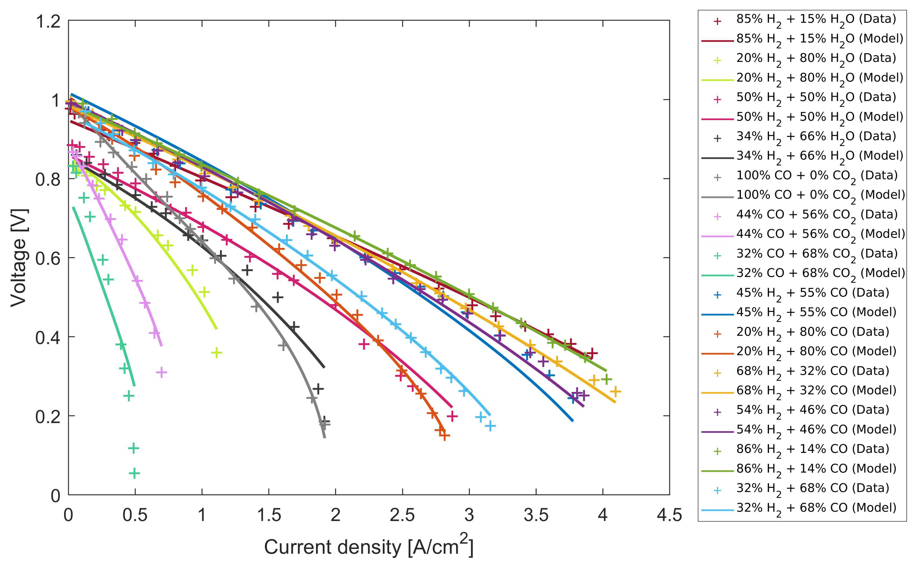
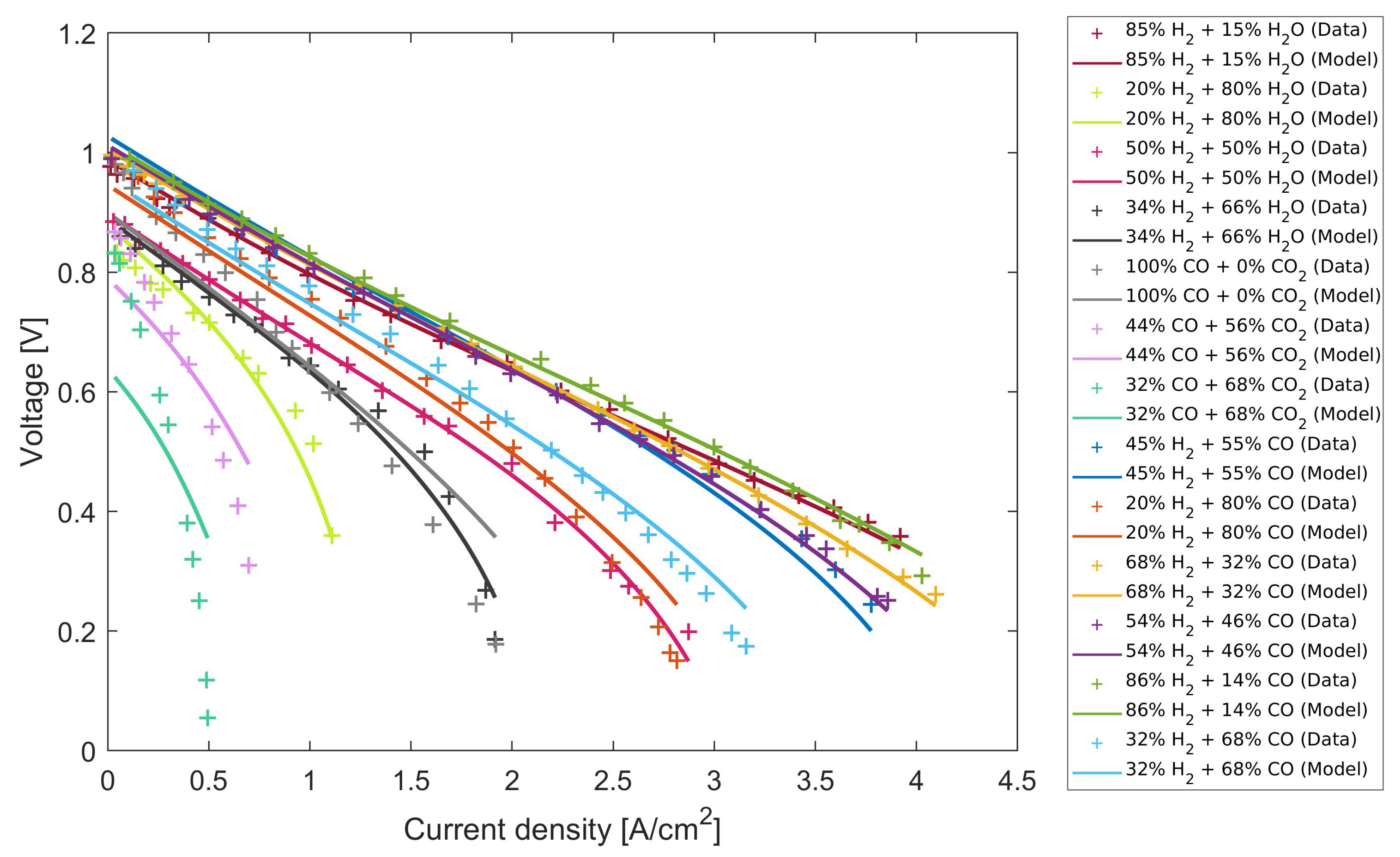
4.1. Calibrating the Model to Experimental Data

The results of the calibrated thermodynamically consistent RDEM show very good agreement with multiple experimental data set used for calibration at once, as shown in Figure 1. The model was calibrated on all 13 polarisation curves obtained with different fuel compositions with a single set of calibration parameter values. Overall, the R${}^2$ obtained in this procedure has a very high value of 0.9976 and the root mean square deviation (RMSD) value is low at only 0.00815. In comparison with other developed models utilising the same set of experimental data set for validation [25,26,39,42,43,44], the newly devised thermodynamically consistent RDEM obtains a significantly better fit quality, as discussed in detail in Section 4.4. The aforementioned quality of replication of experimental data is especially high in the area of activation losses (low current density regions), where the thermodynamically consistent modelling basis taking into account both forward and backward reactions plays an instrumental role in an appropriate description of the underlying phenomena. Additionally, the results also clearly indicate that the majority of the small deviations between experimental data and the output of the model are in the area of concentration losses (high current density region) where the model’s dimensionality plays an important role due to the channel/rib distributions and ratios, which are not taken into account in this work for the sole purpose of achieving a low computational burden due to intended application of the model. This reasoning is confirmed by higher but still reasonable deviations from known values from the literature (

Table A1. List of model calibration parameters obtained from the literature.

Parameter	Value	Units	Description	Source
d${}_{{cl}_c}$	20	$\mathsf{\mu }$m	Thickness of interlayer	[45]
d${}_{{cl}_a}$	10	$\mathsf{\mu }$m	Thickness of interlayer	[45]
S	1.1	cm${}^2$	Effective electrode area	[45]
$ϵ$	0.54	unitless	Porosity	[45]
$\tau$	[ here. 4.89–9]	unitless	Tortuosity	[45]
AV	70 × 10${}^6$	m${}^2$m${}^{-3}$	EASA-to-volume-ratio	[59]
K${}_{e{q}_{{\mathrm{H}}_2}}$	1.66 × 10${}^8$	atm${}^{-0.5}$	H_2 equilibrium constant	[32]
K${}_{e{q}_{\mathrm{CO}}}$	1.07 × 10${}^8$	atm${}^{-0.5}$	CO equilibrium constant	[32]
K${}_{{\mathrm{H}}_2}$	2.1 × 10${}^{11}$ RT/F	A/cm${}^2$	Reaction rate H${}_2$	[32]
K${}_{\mathrm{CO}}$	0.84 × 10${}^{11}$ RT/F	A/cm${}^2$	Reaction rate CO	[32]
K${}_{{\mathrm{O}}_2}$	0.25 × 10${}^{10}$RT/F	A/cm${}^2$	Reaction rate O${}_2$	[32]
E${}_{0_{{\mathrm{H}}_2}}$	130,000	units RT	Activation energy H${}_2$	[32]
E${}_{0_{\mathrm{CO}}}$	120,000	units RT	Activation energy CO	[32]
E${}_{0_{{\mathrm{O}}_2}}$	120,000	units RT	Activation energy O${}_2$	[32]
D${}_{{\mathrm{H}}_2}$	[3.858–5.677]	cm${}^2$s${}^{-1}$	Difussion coefficient H${}_2$	[45]
D${}_{\mathrm{CO}}$	0.958	cm${}^2$s${}^{-1}$	Difussion coefficient CO	[45]
D${}_{{\mathrm{O}}_2}$	1.9844	cm${}^2$s${}^{-1}$	Difussion coefficient O${}_2$	[58]

) of the calibration parameters for diffusion coefficients, which can be observed in

Table 2. List of model calibration parameters and their values.

Parameter	Value	Units	Description
K${}_{{\mathrm{H}}_2}$	1.9284 × 10${}^{11}$ RT/F	A/cm${}^2$	Reaction rate H${}_2$
K${}_{\mathrm{CO}}$	0.7534 × 10${}^{11}$ RT/F	A/cm${}^2$	Reaction rate CO
K${}_{{\mathrm{O}}_2}$	0.21697 × 10${}^{10}$ RT/F	A/cm${}^2$	Reaction rate O${}_2$
E${}_{0_{{\mathrm{H}}_2}}$	136,167	units RT	Activation energy H${}_2$
E${}_{0_{\mathrm{CO}}}$	118,311	units RT	Activation energy CO
E${}_{0_{{\mathrm{O}}_2}}$	113,149	units RT	Activation energy O${}_2$
D${}_{{\mathrm{H}}_2}$	6.3843	cm${}^2$s${}^{-1}$	Difussion coefficient H${}_2$
D${}_{\mathrm{CO}}$	1.2438	cm${}^2$s${}^{-1}$	Difussion coefficient CO
D${}_{{\mathrm{O}}_2}$	0.7457	cm${}^2$s${}^{-1}$	Difussion coefficient O${}_2$

.

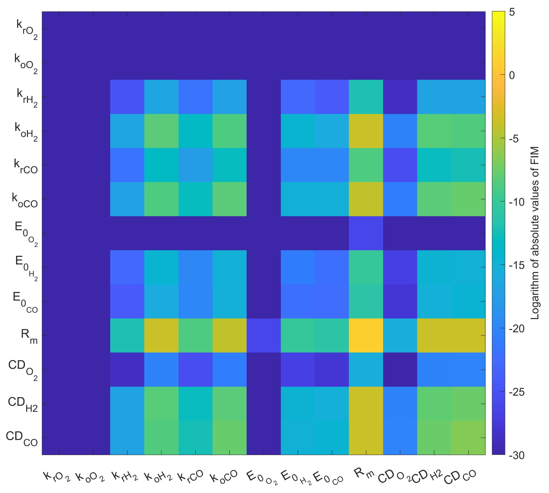
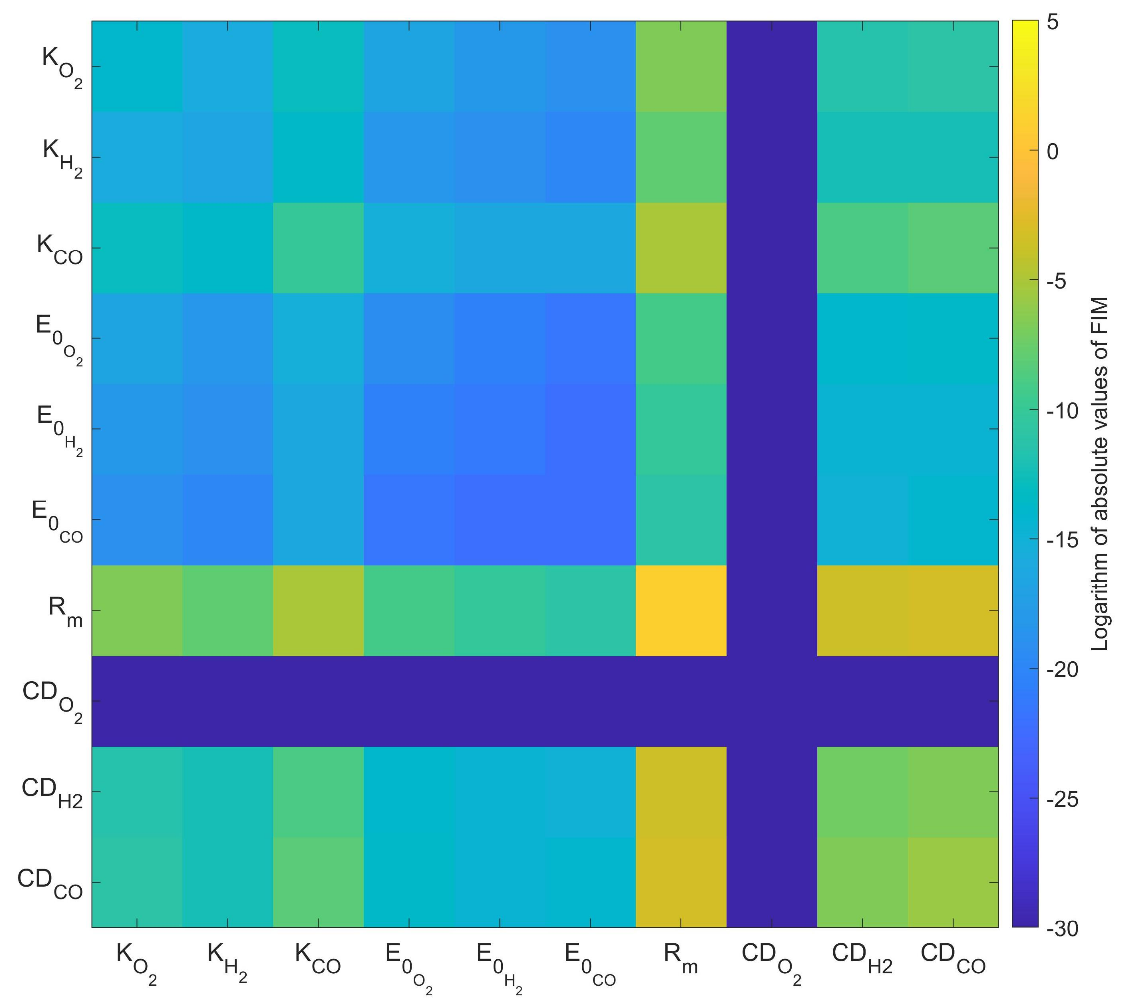
4.2. Parameter Sensitivity and the Standard Error of Parameter Values

The goodness of fit provides us with the information of how accurately the model replicates the training data set. It should be noted, though, that achieving a high goodness of fit does not necessary mean that the calibration parameter values are well defined, as each individual experimental data set possesses only a particular amount of information about the individual calibration parameters, which in return defines both parameter sensitivity and the standard error of the parameter’s values. The results of the FIM analysis are presented in Figure 2. After careful observation, it can be noticed that the cathode parameters are not uniquely determinable on the given data set. The reasoning for this behaviour can be explained by the fact that the experiments were carried out with a very high volume flow and thus stoichiometry, which leads to the decreased influence of these parameters on the overall output of the model. The other calibration parameter values are relatively well defined on the given data set, with the membrane ohmic resistivity being the best defined one. The latter is to be expected since the membrane ohmic resistivity has a linear dependence on the influential operating parameters and, as such, is easier to be determined in comparison with the other calibration parameters, which have highly non-linear contributions to the voltage output of the model. The FIM of results obtained is nearly singular and thus potential reductions of the model should be only considered if the model is utilised in these or similar operating conditions, as is shown.

Nonetheless, the inverse of the FIM can be obtained. Using the correlation between the variance and the standard error, the latter can be obtained for each individual calibration parameter. The results obtained are as follows:

$$\begin{array}{cc}\hfill {\mathbf{\Sigma }}_{\mathbf{\theta }}& ={\left[\begin{array}{cccccccc}{k}_{r_{{\mathrm{O}}_2}}& k_{o_{{\mathrm{O}}_2}}& k_{o_{\mathrm{CO}}}& k_{r_{\mathrm{CO}}}& k_{o_{{\mathrm{H}}_2}}& k_{r_{{\mathrm{H}}_2}}& E_{0_{{\mathrm{O}}_2}}& \dots \\ \dots & E_{0_{\mathrm{CO}}}& E_{0_{{\mathrm{H}}_2}}& R& C{D}_{{\mathrm{O}}_2}& C{D}_{\mathrm{CO}}& C{D}_{{\mathrm{H}}_2}\end{array}\right]}^T\hfill \\ & ={\left[\begin{array}{cccccccc}4.34\times {10}^7& 4.34\times {10}^7& 3.717& 3.717& 7.327& 7.327& 6.43\times {10}^6& \dots \\ \dots & 9.33\times {10}^4& 2.468& 0.2713& 5.812\times {10}^2& 0.4224& 0.8044\end{array}\right]}^T\hfill \end{array}$$

(55)

and show that the lowest standard errors are obtained for ohmic resistivity and the combined diffusivities of CO and H${}_2$, while they are significantly higher for the reaction rate parameters. Parameters that have a high standard error, namely the reaction rates on the cathode $k_{RDC}$, $k_{OXC}$ are hard to uniquely determine. This can be due to the fact that their influence on the output of the model is under the given operating conditions less significant or because they cannot be uniquely determined due to the calibration parameters’ mathematical inter-connectivity. In both cases, it is completely meaningful to propose the following reduction in the set of calibration parameters based on physical reasoning:

$${\mathrm{e}}^{-{\alpha }_c·ln\left(\frac{k_{RDC}}{k_{OXC}}\right)}{k}_{RDC}\to K_{O_2},$$

(56)

since for a common cathode material, the dissociation of adsorbed oxygen molecules is the rate-determining electrochemical reaction step [57]. Furthermore, analogue reductions can also be performed for both electrochemical co-oxidations on the anode side, thus replacing $k_{o_{\mathrm{CO}}}$, $k_{r_{\mathrm{CO}}}$, $k_{o_{{\mathrm{H}}_2}}$, and $k_{r_{{\mathrm{H}}_2}}$ with $K_{CO}$ and $K_{H_2}$. The aforementioned reductions lead to a reduced set of calibration parameters, which are more uniquely identifiable. This can be observed when comparing Figure 2 and Figure 3, where the FIM in Figure 2 has smaller values of FIM and thus higher standard errors in comparison with the Figure 3, which was obtained with the reduced set of calibration parameters, where the values of FIM and are significantly larger and thus the standard errors are lower. As before, these are obtained using the inverse of the FIM and the correlation between variance and the standard error.

The obtained results can be written as follows:

$$\begin{array}{cc}\hfill {\mathbf{\Sigma }}_{\mathbf{\theta }}& ={\left[\begin{array}{cccccc}{K}_{{\mathrm{O}}_2}& K_{{\mathrm{H}}_2}& K_{\mathrm{CO}}& E_{0_{{\mathrm{O}}_2}}& E_{{\mathrm{H}}_2}^0& \dots \\ \dots & E_{\mathrm{CO}}^0& R& C{D}_{{\mathrm{O}}_2}& C{D}_{\mathrm{CO}}& C{D}_{{\mathrm{H}}_2}\end{array}\right]}^T\hfill \\ & ={\left[\begin{array}{cccccc}0.8139& 2.206& 3.642& 1.896& 4.596& \dots \\ \dots & 11.56& 0.2713& 2.076\times {10}^2& 0.3376& 0.5100\end{array}\right]}^T.\hfill \end{array}$$

(57)

This confirms the higher unique identifiability of the calibration parameters. However, due to the reciprocity of estimator variance and the FIM, the increase in the FIM and, thus, information corresponds to the decrease in the variance and consequentially in the standard error. Furthermore, since the performed reduction is physically meaningful, the increase in the model output deviation from the experimental data is small, increasing the RMSD from 0.00815 to 0.0116 and decreasing the R${}^2$ value from 0.9976 to a still extremely high value of 0.9952. Based on the encouraging results of this analysis, the reduced version of the model was utilised in the rest of the performed tests.

Validation with Known Values of Calibration Parameters from the Literature

The reduced modelling basis obtained in the previous subsection is still thermodynamically consistent due to the physical reasoning of the reduction. Therefore, the model should return meaningful results when parametrised with known data from the literature. To test this, the values for reaction rates were taken from [32], the activation energies were taken from [32], and the diffusivities for each individual species were taken from [58]. Their values are presented in Appendix B, and as explained in the Section 3.4, they were used as a basis for the calibration procedure. However, even without using the calibration procedure, the model, using these values, achieved good agreement with the experimental data, with an R${}^2$ value of 0.9853 and an RMSD value of 0.0202, as shown in Figure 4. Therefore, the modelling framework is fully capable of utilising known parameter values from the literature for the reaction rates and the activation energies to produce physically meaningful results, which is a clear merit of this system level model. It should be pointed out that, if the model is utilised under untypical operating conditions, it could generate a higher error, as discussed in more detail in Appendix A.

4.3. Extrapolation Validation

Besides the possibility of adequately simulating the operating points outside of the calibration space of parameters, the enhanced extrapolation capabilities together with the good prediction capabilities and the generality of the model enable the use of significantly smaller data sets to determine the calibration parameters values with a low standard error. With the aim of testing the prediction and extrapolation capabilities of the model, the experimental data set was divided into a training data set and a validation data set. For the first test, the polarisation curves numbered 1 to 6 in Table 1 were used as the training data set and the polarisation curves from numbered 7 to 13 were used as the validation data set. In the second test, the last seven polarisation curves were used for training and the first six were used for validation.

The results of the first test of extrapolation validation are shown in Figure 5 and exhibit a slightly higher R${}^2$ value of 0.9982 in comparison with using all available experimental data, with a corresponding RMSD value of 0.007337 for the training data set and an R${}^2$ value of 0.9908 with a corresponding RMSD value of 0.1546 for the validation data set. An in depth analysis reveals slightly higher RMSD values for the H${}_2$ and H${}_2$O polarisation curves of 0.07439 and even a bit higher RMSD value for the CO and CO${}_2$ polarisation curves of 0.2365 in comparison with the trained values of 0.0108 and 0.0156. This is confirmed with lower R${}^2$ values of 0.9974 for the H${}_2$ and H${}_2$O polarisation curves and of 0.9832 for the CO and CO${}_2$ polarisation curves, which is an expected result based on the modelling assumptions and modelling depth of the framework at hand, especially since most of the deviations comes from the high current density region, where the model’s reduced dimensionality begins to show its limits.

To confirm the results obtained the extrapolation capabilities of the thermodynamically consistent RDEM were also assessed in the opposite direction with the second test. There, the model was calibrated on the polarisation curves obtained with mixtures of either H${}_2$ and H${}_2$O, or CO and CO${}_2$ and then used to simulate the six polarisation curves that were obtained with different mixtures of CO and H${}_2$. The results presented in Figure 6 show a very good replication of the experimental data for both cases. For the training data set, the R${}^2$ value is 0.9923 and the RMSD value is 0.01414, which confirms a better fit of the model to the experimental data in comparison with the first analysed case. The analysis of the extrapolation capabilities show extremely good results with an R${}^2$ value of 0.9974 and am RMSD value of 0.004014. The presented results confirm that the model is not only very accurate but also exhibits extremely good extrapolation and predictive capabilities.

4.4. Comparison with Other Known Models from the Literature

A literature review showed that several computationally fast, reduced dimensionality models are used in the system level applications. As the performance of these reduced dimensionality models depends also on the experimental data set utilised in the calibration procedure, it is meaningful to compare only the models that were validated and trained on the same experimental data set. Therefore, the comparison of the newly developed thermodynamically consistent multi-species electrochemical model was carried out with the six system level models [25,26,39,42,43,44], which utilised the experimental data provided in [45] as their validation data set. For each of the models, the fit quality was assessed by means of an RMSD value calculated on each of the polarisation curves. The results obtained in the scope of this analysis are presented in

Table 3. Comparison of RMSD values for individual polarisation curves obtained with known system level models of similar modelling depth from the literature.

Composition [%]	[43]	[42]	[44]	[25]	[39]	[26]	Our Model
85 H2-15 H2O	0.1099	0.1516	0.1587	/	0.1755	0.1361	0.02175
50 H2-50 H2O	0.1189	0.1010	0.1074	0.1529	0.1901	0.1928	0.04116
34 H2-66 H2O	0.1228	0.09958	0.1761	0.1399	0.2150	0.2114	0.02212
20 H2-80 H2O	0.1483	0.1813	0.3999	0.1625	0.1499	0.2041	0.04556
97 CO-3 CO2	0.1507	0.1572	0.1285	/	0.2267	/	0.02556
44 CO-56 CO2	0.2158	0.1731	0.1663	/	0.1634	/	0.03037
32 CO-68 CO2	0.1491	0.2629	0.3245	/	0.3714	/	0.1208
86 H2-14 CO	0.1541	0.1224	0.1593	/	0.3025	/	0.04165
68 H2-32 CO	/	0.3464	0.1532	/	0.2076	/	0.03675
54 H2-46 CO	/	/	/	/	0.2298	/	0.03629
45 H2-55 CO	0.1794	0.1314	0.1339	/	0.3478	/	0.01652
32 H2-68 CO	/	0.1780	0.3140	/	0.1771	/	0.02496
20 H2-80 CO	0.2914	0.1753	0.2229	/	0.2648	/	0.02117

. The results show that the newly developed thermodynamically consistent multi-species electrochemical model has the smallest deviations from the validation data set. The highest deviation is achieved when the SOFC is fuelled with 32% of CO and 68% of the CO${}_2$, where the model obtained in [43] obtains comparable RMSD values. For all of the other operating points, the newly developed model has smaller RMSD values than all known system level models from the literature, clearly positioning it as the current state-of-the-art.

5. Conclusions

The presented study fills the knowledge gap in the area of thermodynamically consistent reduced dimensionality multi-species electrochemical models. It provides, for the first time, the closed-form solution for the anode over-potential of multiple species with the electrochemical co-oxidation of CO and H${}_2$ and thus provides an easily invertible solution for the voltage or the net current of fuel cells fuelled with multi-species fuel. The expression obtained is valid for all current density regions and consistently features the reduction and oxidation reactions for both the cathode and the anode side of the SOFC. The presented results show the validation process of the model on polarisation curves obtained with different fuel mixtures resulting in an extremely high R${}^2$ value of 0.9952, thus confirming the capability of the newly developed model to replicate experimental data. A fitness function analysis further confirms that the thermodynamically consistent multi-species electrochemical model exhibits very good extrapolation capabilities for operating conditions outside the calibrated variation space of the parameters, thus proving its robustness. The model under these tests achieves an R${}^2$ value of 0.9994 when trained on the CO/CO${}_2$ and H${}_2$/H${}_2$O individually and validated on the mixture of CO and H${}_2$, and an R${}^2$ value of 0.9908 when trained on the mixture of CO and H${}_2$ and validated on the individual fuel. Furthermore, owing to its thermodynamically consistent basis, the modelling framework can be parametrised using solely known values of the calibration parameters from the literature, resulting in an extremely high R${}^2$ value of 0.9853 when validated on all 13 polarisation curves obtained with different fuel mixtures. The R${}^2$ value obtained is especially high for any non-calibrated reduced dimensionality model. Furthermore, the newly developed model obtains in comparison with the other known models from the literature on average for smaller RMSD values on the training data set. Therefore, the proposed modelling framework represents significant progress in the area of system-level electrochemical models for control applications. Furthermore, it can serve as a model basis of digital twins and model-based DoEs as well assists in the model supported development of SOFC. These key features confirm the modelling framework as a beyond state-of-the-art tool for the model-endorsed development of advanced clean energy conversion technologies. As such, it offers a good basis for the development of a tool for combined service and lifetime optimisations, when coupled with the intertwined degradation modelling framework, which proves to be incredibly demanding task and will be tackled in future research.

References

1. Bridgwater, A. The technical and economic feasibility of biomass gasification for power generation. Fuel 1995, 74, 631–653. [Google Scholar] [CrossRef]
2. Samiran, N.A.; Jaafar, M.N.M.; Ng, J.H.; Lam, S.S.; Chong, C.T. Progress in biomass gasification technique—With focus on Malaysian palm biomass for syngas production. Renew. Sustain. Energy Rev. 2016, 62, 1047–1062. [Google Scholar] [CrossRef]
3. Di Blasi, C. Combustion and gasification rates of lignocellulosic chars. Prog. Energy Combust. Sci. 2009, 35, 121–140. [Google Scholar] [CrossRef]
4. de Lasa, H.; Salaices, E.; Mazumder, J.; Lucky, R. Catalytic Steam Gasification of Biomass: Catalysts, Thermodynamics and Kinetics. Chem. Rev. 2011, 111, 5404–5433. [Google Scholar] [CrossRef]
5. Devi, L.; Ptasinski, K.J.; Janssen, F.J. A review of the primary measures for tar elimination in biomass gasification processes. Biomass Bioenergy 2003, 24, 125–140. [Google Scholar] [CrossRef]
6. Holladay, J.; Hu, J.; King, D.; Wang, Y. An overview of hydrogen production technologies. Catal. Today 2009, 139, 244–260. [Google Scholar] [CrossRef]
7. Kravos, A.; Seljak, T.; Rodman Oprešnik, S.; Katrašnik, T. Operational stability of a spark ignition engine fuelled by low H2 content synthesis gas: Thermodynamic analysis of combustion and pollutants formation. Fuel 2020, 261, 116457. [Google Scholar] [CrossRef]
8. Marcantonio, V.; Del Zotto, L.; Ouweltjes, J.P.; Bocci, E. Main issues of the impact of tar, H2S, HCl and alkali metal from biomass-gasification derived syngas on the SOFC anode and the related gas cleaning technologies for feeding a SOFC system: A review. Int. J. Hydrog. Energy 2021, 47, 517–539. [Google Scholar] [CrossRef]
9. Arriagada, J.; Olausson, P.; Selimovic, A. Artificial neural network simulator for SOFC performance prediction. J. Power Sources 2002, 112, 54–60. [Google Scholar] [CrossRef]
10. Entchev, E.; Yang, L. Application of adaptive neuro-fuzzy inference system techniques and artificial neural networks to predict solid oxide fuel cell performance in residential microgeneration installation. J. Power Sources 2007, 170, 122–129. [Google Scholar] [CrossRef]
11. Huo, H.B.; Zhu, X.J.; Hu, W.Q.; Tu, H.Y.; Li, J.; Yang, J. Nonlinear model predictive control of SOFC based on a Hammerstein model. J. Power Sources 2008, 185, 338–344. [Google Scholar] [CrossRef]
12. Bellman, R.E. Dynamic Programming; Princeton University Press: Princeton, NJ, USA, 1957. [Google Scholar]
13. Kravos, A.; Ritzberger, D.; Tavčar, G.; Hametner, C.; Jakubek, S.; Katrašnik, T. Thermodynamically consistent reduced dimensionality electrochemical model for proton exchange membrane fuel cell performance modelling and control. J. Power Sources 2020, 454, 227930. [Google Scholar] [CrossRef]
14. Kulikovsky, A.A. A Physically–Based Analytical Polarization Curve of a PEM Fuel Cell. J. Electrochem. Soc. 2013, 161, F263–F270. [Google Scholar] [CrossRef]
15. Gu, W.; Baker, D.R.; Liu, Y.; Gasteiger, H.A. Proton exchange membrane fuel cell (PEMFC) down-the-channel performance model. In Handbook of Fuel Cells; American Cancer Society: Atlanta, GA, USA, 2010. [Google Scholar] [CrossRef]
16. Mueller, F.; Brouwer, J.; Jabbari, F.; Samuelsen, S. Dynamic Simulation of an Integrated Solid Oxide Fuel Cell System Including Current-Based Fuel Flow Control. J. Fuel Cell Sci. Technol. 2005, 3, 144–154. [Google Scholar] [CrossRef]
17. Wu, C.C.; Chen, T.L. Dynamic Modeling of a Parallel-Connected Solid Oxide Fuel Cell Stack System. Energies 2020, 13, 501. [Google Scholar] [CrossRef] [Green Version]
18. Chan, S.; Khor, K.; Xia, Z. A complete polarization model of a solid oxide fuel cell and its sensitivity to the change of cell component thickness. J. Power Sources 2001, 93, 130–140. [Google Scholar] [CrossRef]
19. Dolenc, B.; Boskoski, P.; Pohjoranta, A.; Noponen, M.; Juricic, D. Hybrid Approach to Remaining Useful Life Prediction of Solid Oxide Fuel Cell Stack. ECS Trans. 2017, 78, 2251–2264. [Google Scholar] [CrossRef]
20. DiGiuseppe, G. An Electrochemical Model of a Solid Oxide Fuel Cell Using Experimental Data for Validation of Material Properties. In Proceedings of the ASME 2010 8th International Fuel Cell Science, Engineering and Technology Conference: Volume 2, Brooklyn, NY, USA, 14–16 June 2010; pp. 193–203. [Google Scholar] [CrossRef]
21. Siegel, J.B.; Wang, Y.; Stefanopoulou, A.G.; McCain, B.A. Comparison of SOFC and PEM Fuel Cell Hybrid Power Management Strategies for Mobile Robots. In Proceedings of the 2015 IEEE Vehicle Power and Propulsion Conference (VPPC), Montreal, QC, Canada, 19–22 October 2015; pp. 1–6. [Google Scholar] [CrossRef]
22. Dolenc, B.; Boskoski, P.; Stepancic, M.; Pohjoranta, A.; Juricic, D. State of health estimation and remaining useful life prediction of solid oxide fuel cell stack. Energy Convers. Manag. 2017, 148, 993–1002. [Google Scholar] [CrossRef]
23. Bianchi, F.R.; Bosio, B.; Baldinelli, A.; Barelli, L. Optimization of a Reference Kinetic Model for Solid Oxide Fuel Cells. Catalysts 2020, 10, 104. [Google Scholar] [CrossRef] [Green Version]
24. Das, T.; Narayanan, S.; Mukherjee, R. Model Based Characterization of Transient Response of a Solid Oxide Fuel Cell System. In ASME International Mechanical Engineering Congress and Exposition, Seattle, WA, USA, 11–15 November 2017, Proceedings of the Volume 6: Energy Systems: Analysis, Thermodynamics and Sustainability; ASME: New York, NY, USA, 2007; pp. 655–664. [Google Scholar] [CrossRef] [Green Version]
25. Lee, W.Y.; Wee, D.; Ghoniem, A.F. An improved one-dimensional membrane-electrode assembly model to predict the performance of solid oxide fuel cell including the limiting current density. J. Power Sources 2009, 186, 417–427. [Google Scholar] [CrossRef]
26. Tabish, A.; Patel, H.; Chundru, P.; Stam, J.; Aravind, P. An SOFC anode model using TPB-based kinetics. Int. J. Hydrog. Energy 2020, 45, 27563–27574. [Google Scholar] [CrossRef]
27. Zhu, H.; Kee, R.; Janardhanan, V.; Deutschmann, O.; Goodwin, D. Modeling Elementary Heterogeneous Chemistry and Electrochemistry in Solid-Oxide Fuel Cells. J. Electrochem. Soc. 2005, 152, A2427. [Google Scholar] [CrossRef] [Green Version]
28. Audasso, E.; Bianchi, F.R.; Bosio, B. 2D Simulation for CH4 Internal Reforming-SOFCs: An Approach to Study Performance Degradation and Optimization. Energies 2020, 13, 4116. [Google Scholar] [CrossRef]
29. Li, P.W.; Chyu, M.K. Electrochemical and Transport Phenomena in Solid Oxide Fuel Cells. J. Heat Transf. 2005, 127, 1344–1362. [Google Scholar] [CrossRef]
30. Nerat, M.; Juricic, D. A comprehensive 3-D modeling of a single planar solid oxide fuel cell. Int. J. Hydrog. Energy 2016, 41, 3613–3627. [Google Scholar] [CrossRef]
31. Zhu, H.; Kee, R.J. A general mathematical model for analyzing the performance of fuel-cell membrane-electrode assemblies. J. Power Sources 2003, 117, 61–74. [Google Scholar] [CrossRef]
32. Suwanwarangkul, R.; Croiset, E.; Entchev, E.; Charojrochkul, S.; Pritzker, M.; Fowler, M.; Douglas, P.; Chewathanakup, S.; Mahaudom, H. Experimental and modeling study of solid oxide fuel cell operating with syngas fuel. J. Power Sources 2006, 161, 308–322. [Google Scholar] [CrossRef]
33. Suwanwarangkul, R.; Croiset, E.; Pritzker, M.; Fowler, M.; Douglas, P.; Entchev, E. Modelling of a cathode-supported tubular solid oxide fuel cell operating with biomass-derived synthesis gas. J. Power Sources 2007, 166, 386–399. [Google Scholar] [CrossRef]
34. Andersson, M.; Yuan, J.; Sundén, B. SOFC modeling considering hydrogen and carbon monoxide as electrochemical reactants. J. Power Sources 2013, 232, 42–54. [Google Scholar] [CrossRef] [Green Version]
35. Nagel, F.P.; Schildhauer, T.J.; Biollaz, S.M.; Wokaun, A. Performance comparison of planar, tubular and Delta8 solid oxide fuel cells using a generalized finite volume model. J. Power Sources 2008, 184, 143–164. [Google Scholar] [CrossRef]
36. Ni, M. Modeling of SOFC running on partially pre-reformed gas mixture. Int. J. Hydrog. Energy 2012, 37, 1731–1745. [Google Scholar] [CrossRef] [Green Version]
37. Ni, M. The effect of electrolyte type on performance of solid oxide fuel cells running on hydrocarbon fuels. Int. J. Hydrog. Energy 2013, 38, 2846–2858. [Google Scholar] [CrossRef] [Green Version]
38. Bao, C.; Wang, Y.; Feng, D.; Jiang, Z.; Zhang, X. Macroscopic modeling of solid oxide fuel cell (SOFC) and model-based control of SOFC and gas turbine hybrid system. Prog. Energy Combust. Sci. 2018, 66, 83–140. [Google Scholar] [CrossRef]
39. Hornbostel, K. Modeling of Solid Oxide Fuel Cell Performance with Coal Gasification. Ph.D. Thesis, Massachusetts Institute of Technology, Cambridge, MA, USA, 2016. [Google Scholar]
40. Bao, C.; Shi, Y.; Croiset, E.; Li, C.; Cai, N. A multi-level simulation platform of natural gas internal reforming solid oxide fuel cell–gas turbine hybrid generation system: Part I. Solid oxide fuel cell model library. J. Power Sources 2010, 195, 4871–4892. [Google Scholar] [CrossRef]
41. Petruzzi, L.; Cocchi, S.; Fineschi, F. A global thermo-electrochemical model for SOFC systems design and engineering. J. Power Sources 2003, 118, 96–107. [Google Scholar] [CrossRef]
42. Bao, C.; Zhang, X. One-Dimensional Macroscopic Model of Solid Oxide Fuel Cell Anode with Analytical Modeling of H2/CO Electrochemical Co-oxidation. Electrochim. Acta 2014, 134, 426–434. [Google Scholar] [CrossRef]
43. Bao, C.; Yixiang, S.; Li, C.; Cai, N.; Su, Q. Mathematical Modeling of Solid Oxide Fuel Cells at High Fuel Utilization Based on Diffusion Equivalent Circuit Model. AIChE J. 2009, 56, 1363–1371. [Google Scholar] [CrossRef]
44. Bao, C.; Jiang, Z.; Zhang, X. Mathematical modeling of synthesis gas fueled electrochemistry and transport including H2/CO co-oxidation and surface diffusion in solid oxide fuel cell. J. Power Sources 2015, 294, 317–332. [Google Scholar] [CrossRef]
45. Jiang, Y.; Virkar, A.V. Fuel Composition and Diluent Effect on Gas Transport and Performance of Anode-Supported SOFCs. J. Electrochem. Soc. 2003, 150, A942. [Google Scholar] [CrossRef]
46. Kravos, A.; Ritzberger, D.; Hametner, C.; Jakubek, S.; Katrašnik, T. Methodology for efficient parametrisation of electrochemical PEMFC model for virtual observers: Model based optimal design of experiments supported by parameter sensitivity analysis. Int. J. Hydrog. Energy 2021, 46, 13832–13844. [Google Scholar] [CrossRef]
47. O’Hayre, R.; Cha, S.; Colella, W.; Prinz, F. Fuel Cell Fundamentals; Wiley: Hoboken, NJ, USA, 2009. [Google Scholar]
48. Mench, M. Fuel Cell Engines; Wiley: Hoboken, NJ, USA, 2008. [Google Scholar]
49. Atkins, P.; De Paula, J.; Keeler, J. Atkins’ Physical Chemistry; Oxford University Press: Oxford, UK, 2018. [Google Scholar]
50. Fornasiero, P.; Graziani, M. Renewable Resources and Renewable Energy: A Global Challenge, 2nd ed.; CRC Press: Boca Raton, FL, USA, 2006. [Google Scholar]
51. Kulikovsky, A. Analytical Modelling of Fuel Cells; Elsevier B.V.: Amsterdam, The Netherlands, 2010. [Google Scholar] [CrossRef]
52. U.S. Patent; Trademark Office. Official Gazette of the United States Patent and Trademark Office: Patents; Number v. 1168, nos. 3-4; U.S. Department of Commerce, Patent and Trademark Office: Washington, DC, USA, 1994. [Google Scholar]
53. Kravos, A.; Kregar, A.; Katrašnik, T. Hybrid Methodology for Efficient on the Fly (Re)Parametrization of Proton Exchange Membrane Fuel Cells Electrochemical Model for Diagnostics and Control Applications. ECS Trans. 2020, 98, 13–24. [Google Scholar] [CrossRef]
54. Kay, S.M. Fundamentals of Statistical Signal Processing; Prentice Hall PTR: Hoboken, NJ, USA, 1993. [Google Scholar]
55. Storn, R.; Price, K. Differential Evolution—A Simple and Efficient Heuristic for Global Optimization over Continuous Spaces. J. Glob. Optim. 1997, 11, 341–359. [Google Scholar] [CrossRef]
56. MATLAB. Optimization Toolbox Release; The MathWorks, Inc.: Natick, MA, USA, 2018. [Google Scholar]
57. Minh, N.Q.; Takahashi, T. Chapter 8—Electrode reaction. In Science and Technology of Ceramic Fuel Cells; Minh, N.Q., Takahashi, T., Eds.; Elsevier Science Ltd.: Oxford, UK, 1995; pp. 199–232. [Google Scholar] [CrossRef]
58. Roberts, R. American Institute of Physics Handbook: 2s. Molecular Diffusion of Gases; A McGraw-Hill Classic Handbook Reissue; McGraw-Hill: New York, NY, USA, 1972. [Google Scholar]
59. Marrero-López, D.; Ruiz-Morales, J.; Peña-Martínez, J.; Canales-Vázquez, J.; Núñez, P. Preparation of thin layer materials with macroporous microstructure for SOFC applications. J. Solid State Chem. 2008, 181, 685–692. [Google Scholar] [CrossRef]
Figure 1. Results of the calibrated model with a single set of calibration parameter values for multiple polarisation curves.
Catalysts 12 00056 g001
Figure 2. The logarithm of the absolute values of the FIM obtained for the model calibrated on the full experimental data set.
Catalysts 12 00056 g002
Figure 3. The logarithm of the absolute values of the FIM obtained for the model calibrated on the full experimental data set with the reduced set of calibration parameters.
Catalysts 12 00056 g003
Figure 4. The results of the model calibrated with known values of calibration parameters from the literature as given in Appendix B for multiple polarisation curves.
Catalysts 12 00056 g004
Figure 5. The first test in the scope of extrapolation validation; the results of the calibrated model on (a) the training data set consisting of the first six polarisation curves and (b) the validation data set consisting of the last seven polarisation curves.
Catalysts 12 00056 g005
Figure 6. The second test in the scope of the extrapolation validation; the results of the calibrated model on (a) the training data set consisting of the last seven polarisation curves and (b) the validation data set consisting of the first six polarisation curves.
Catalysts 12 00056 g006