
The Effect of Different Pretreatment of Chicken Manure for Electricity Generation in Membrane-Less Microbial Fuel Cell


 , , ,
, , ,  ,
,  , and
, and 
Abstract
:1. Introduction
2. Results and Discussion
2.1. Proximate Analysis of Substrates
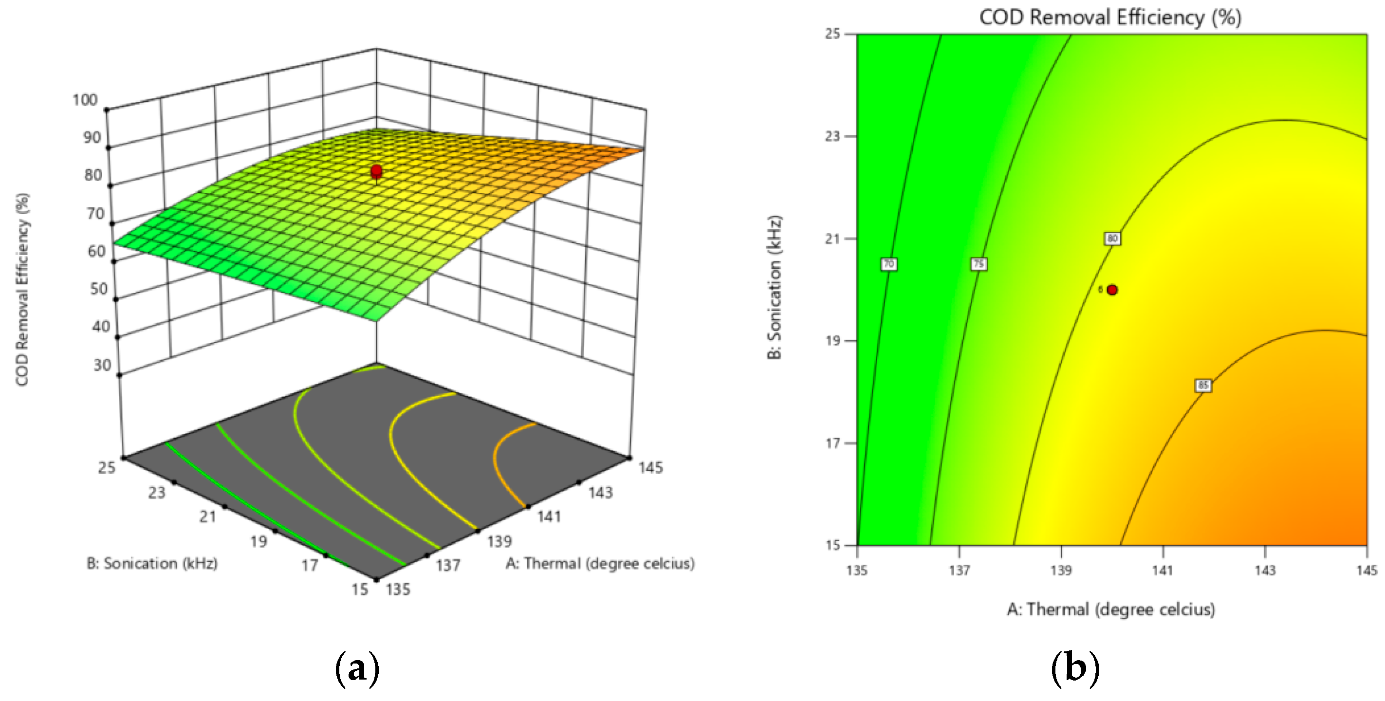
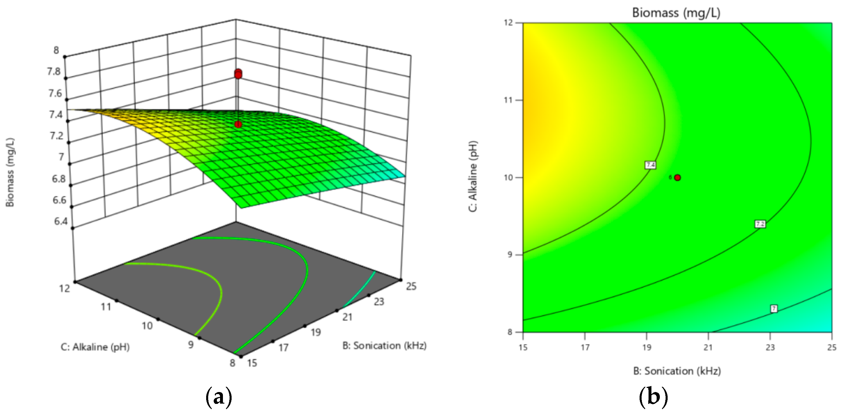
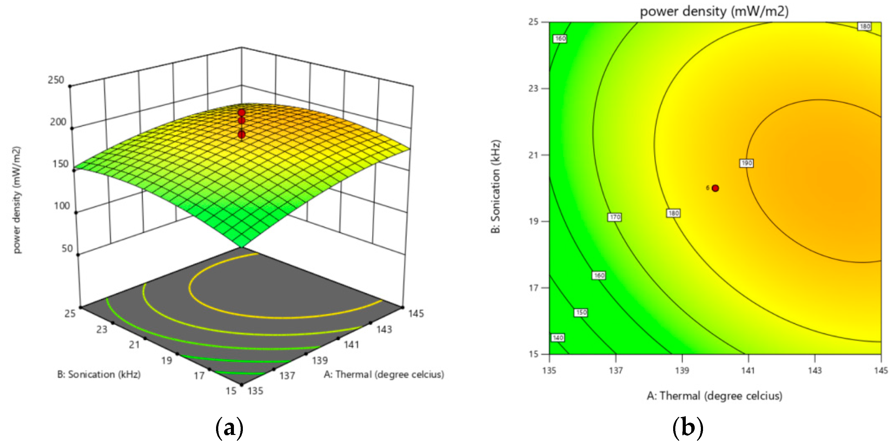
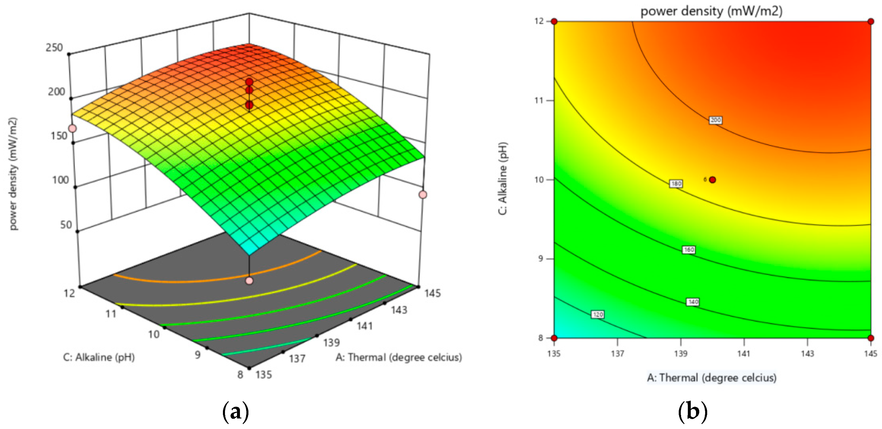
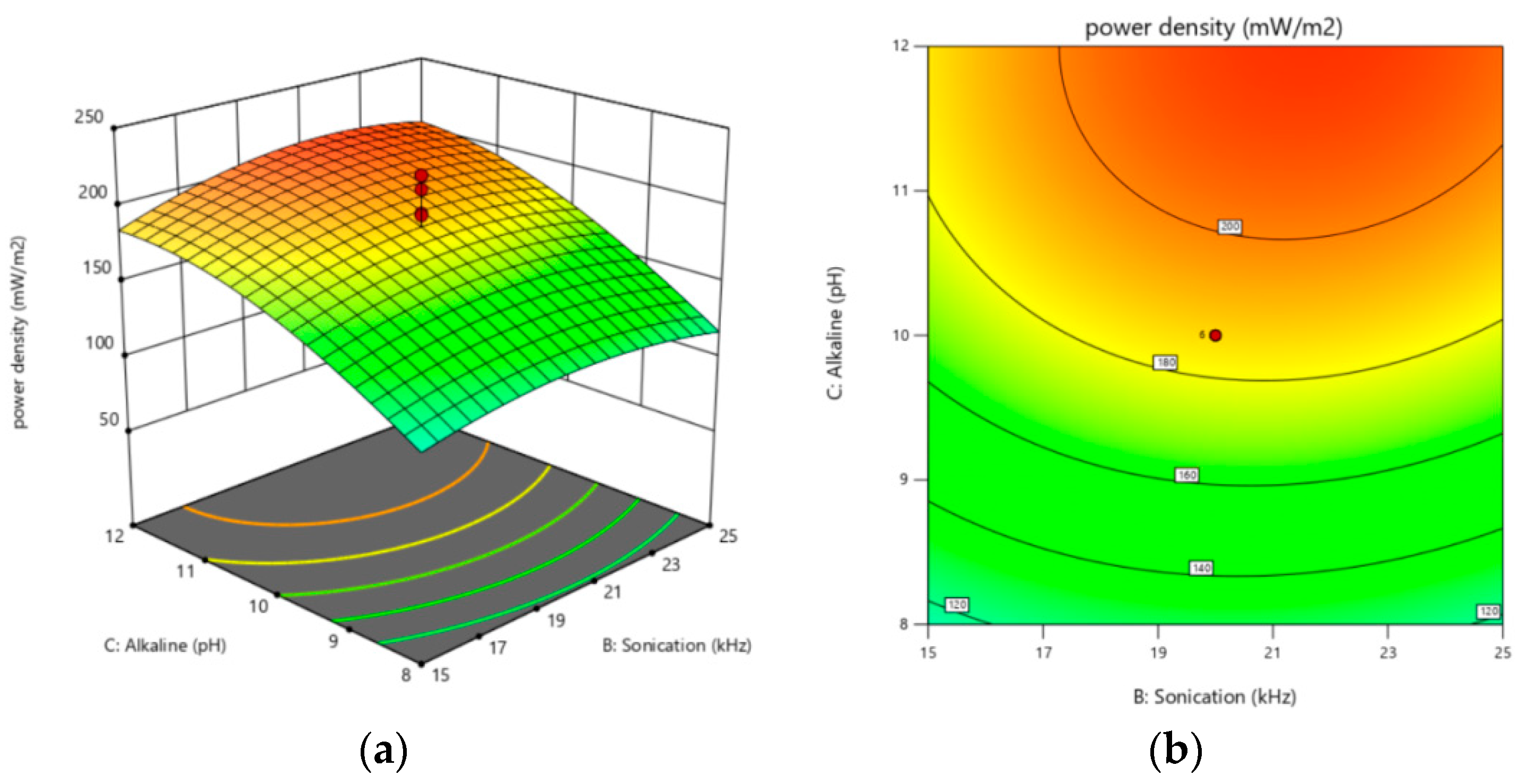
2.2. Optimization of Pretreatment for Electricity Generation Using Response Surface Methodology (RSM) with a CCD
2.2.1. Statistical Analysis and Regression Model
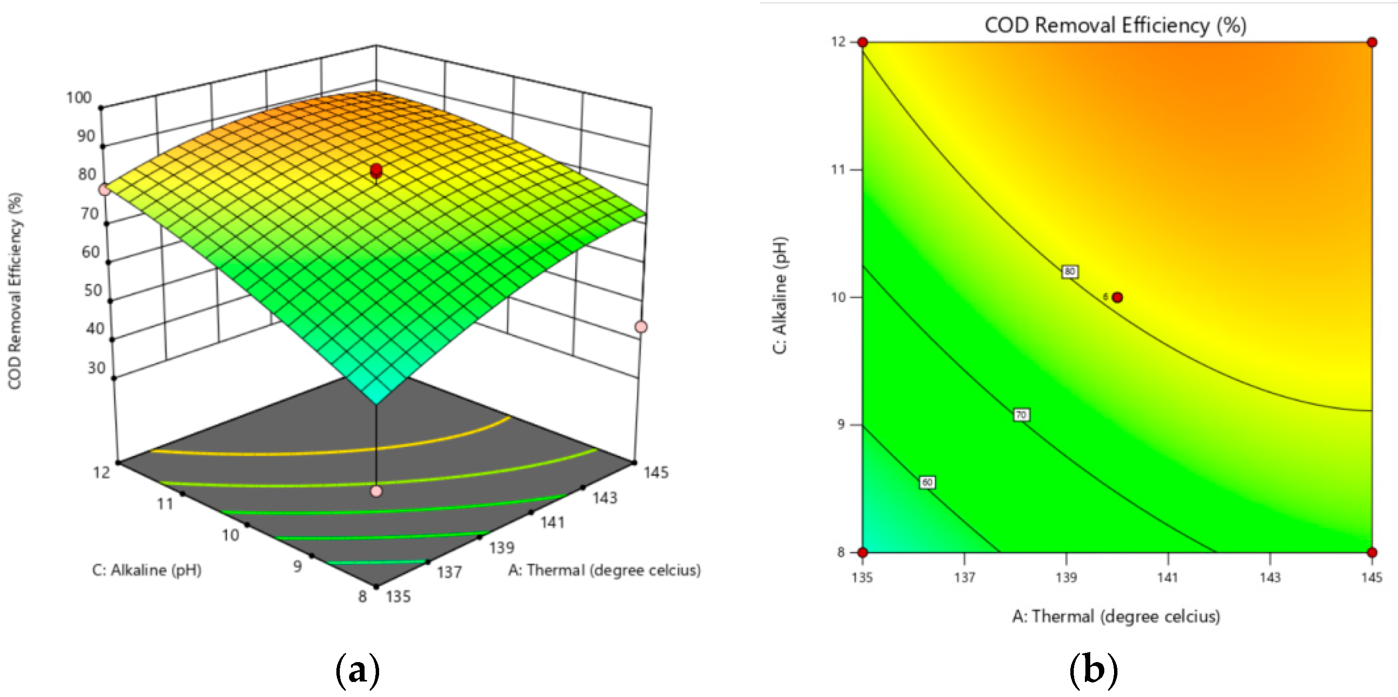
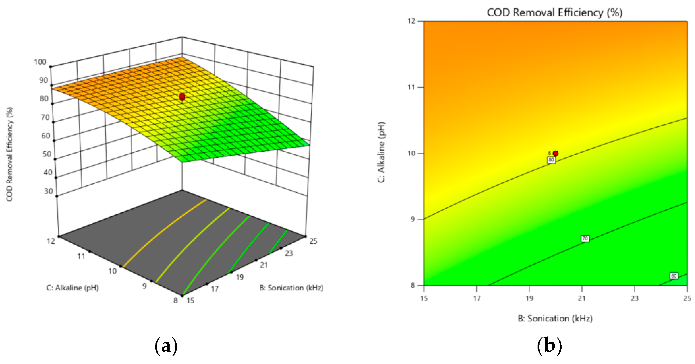
- COD removal efficiency
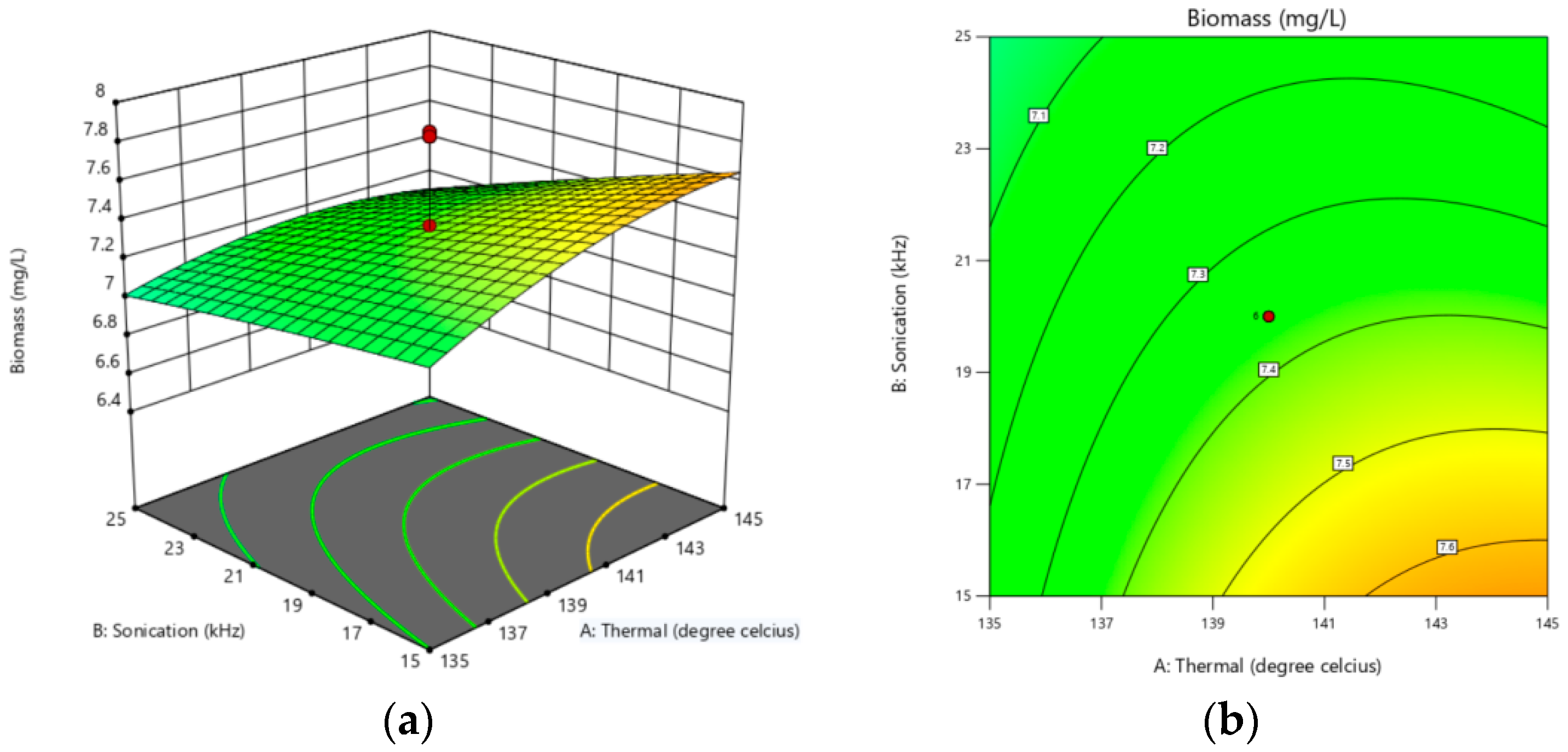
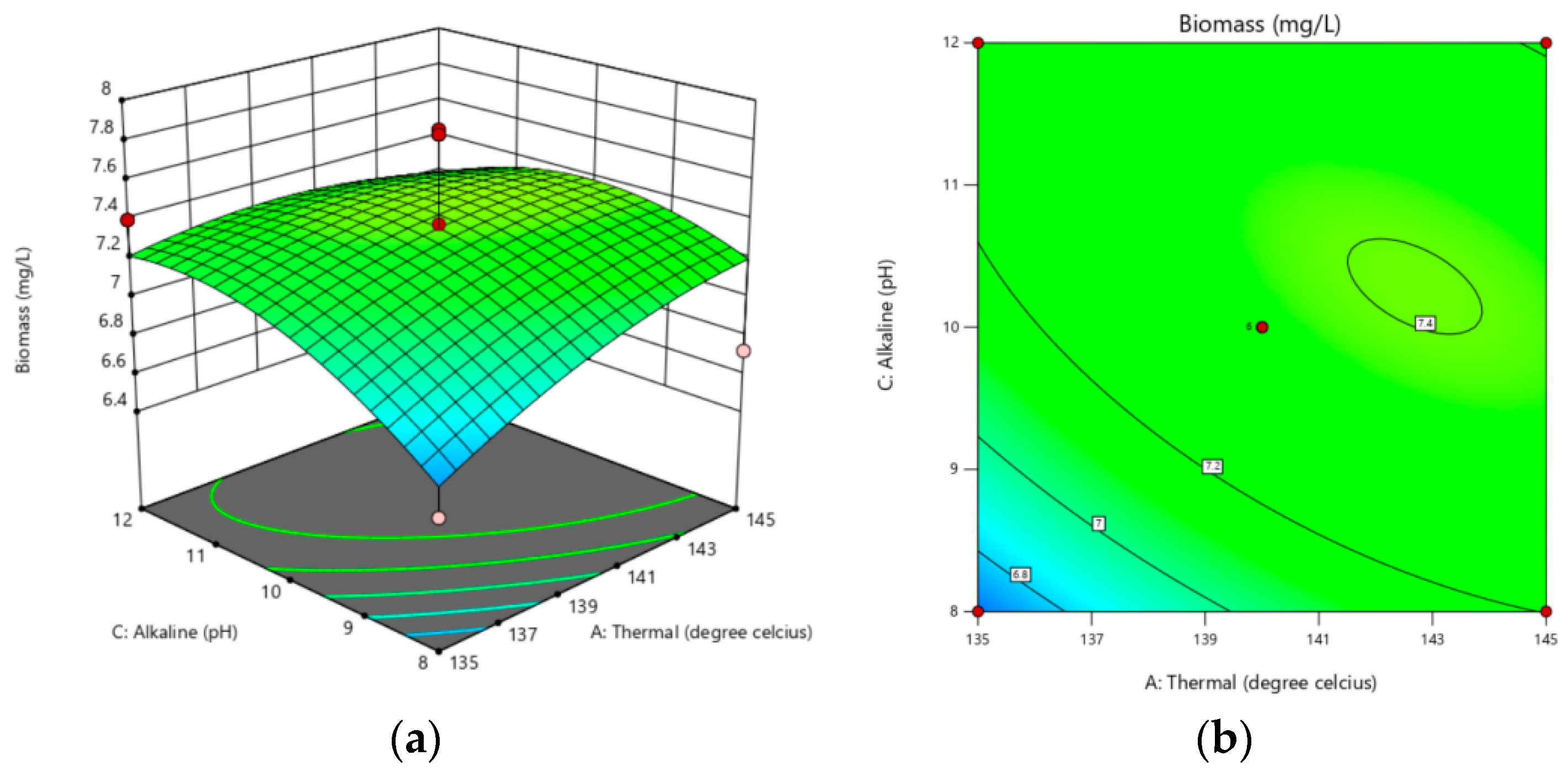
- Biomass
- Power density
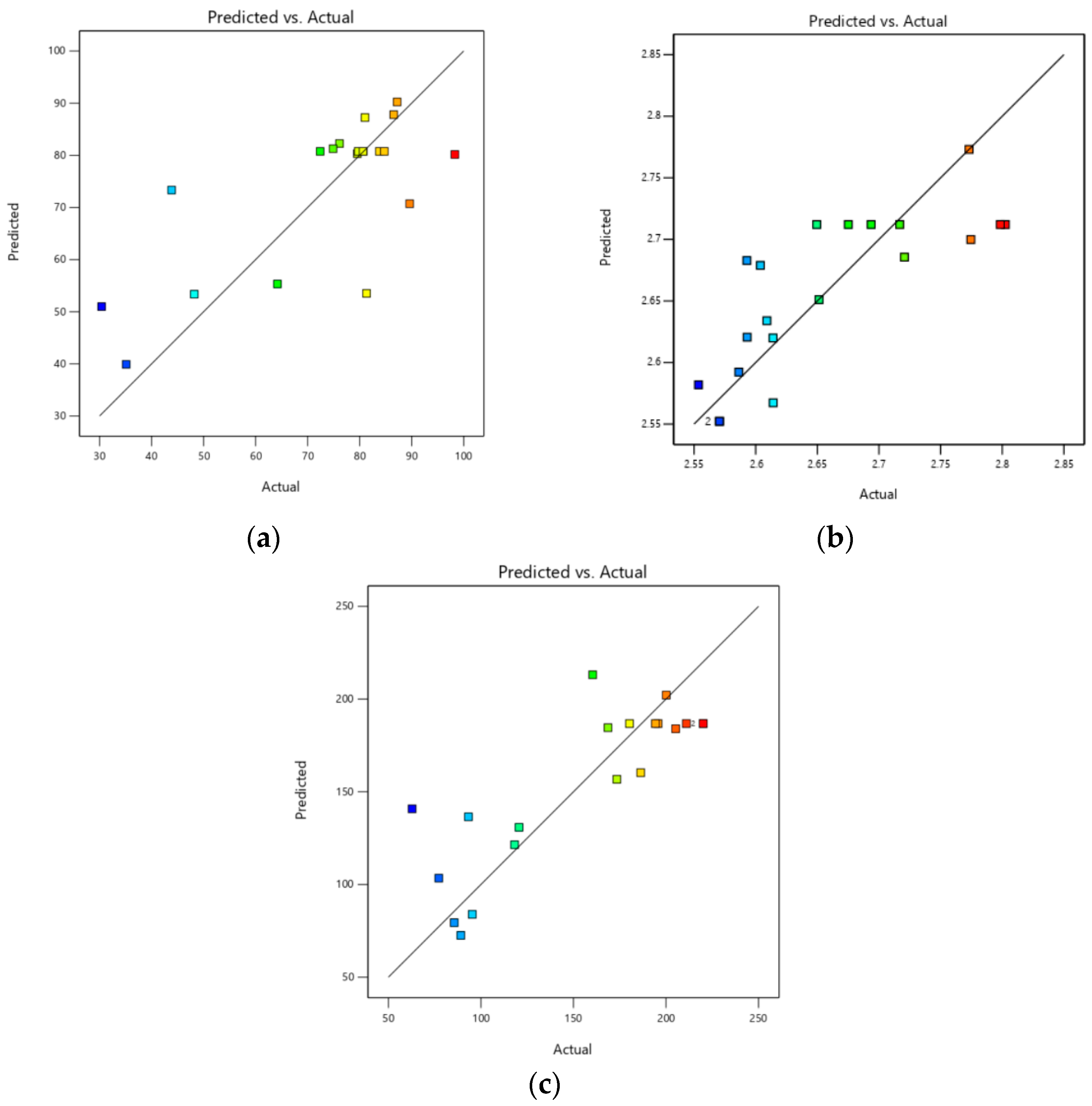
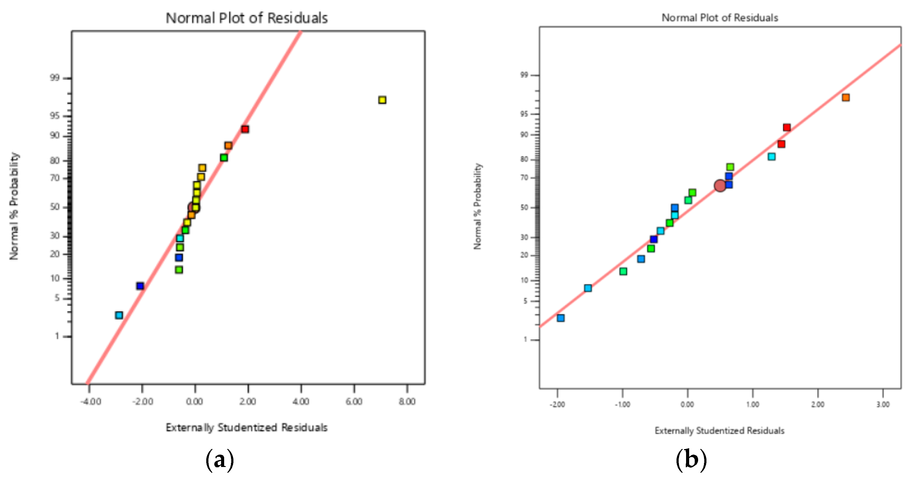
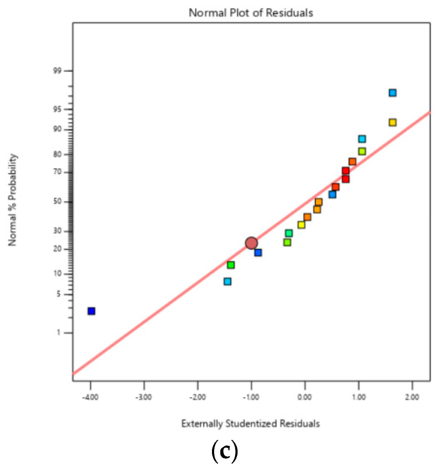
2.2.2. Process and Validation of Models
2.3. ML-MFC Performance
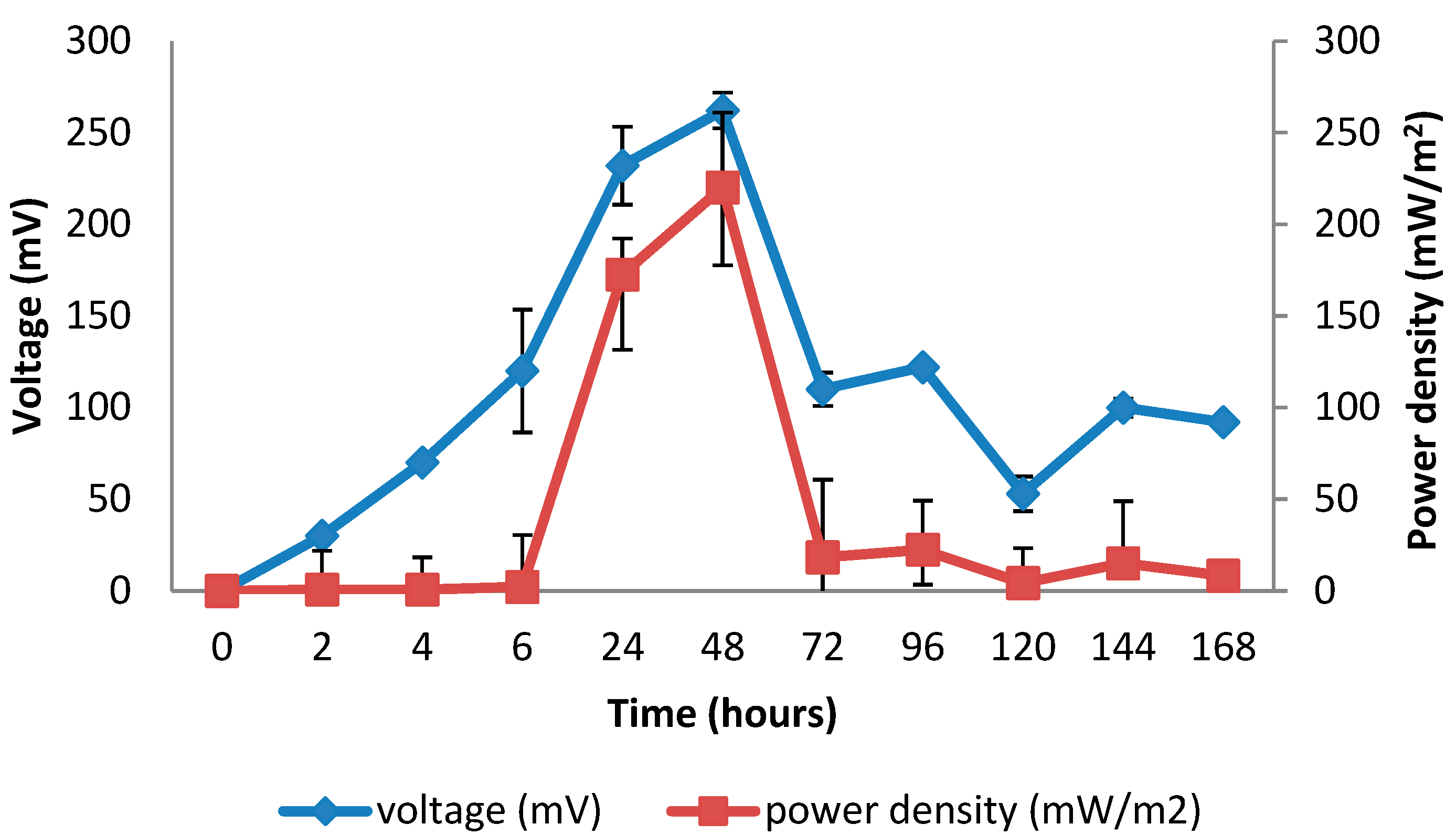
2.3.1. Voltage Generation and Power Density
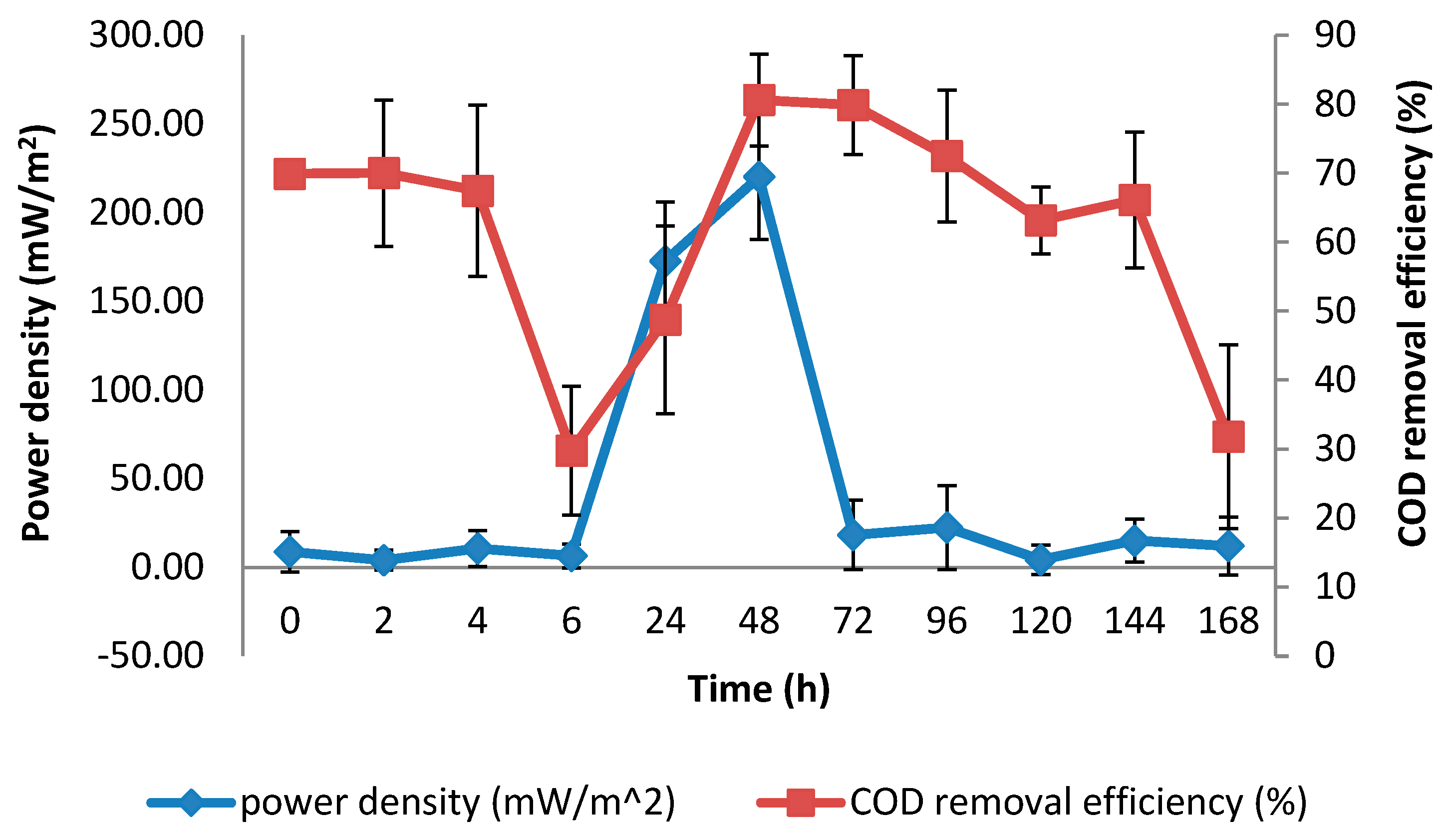
2.3.2. Power Density, COD Removal Efficiency, and Biomass
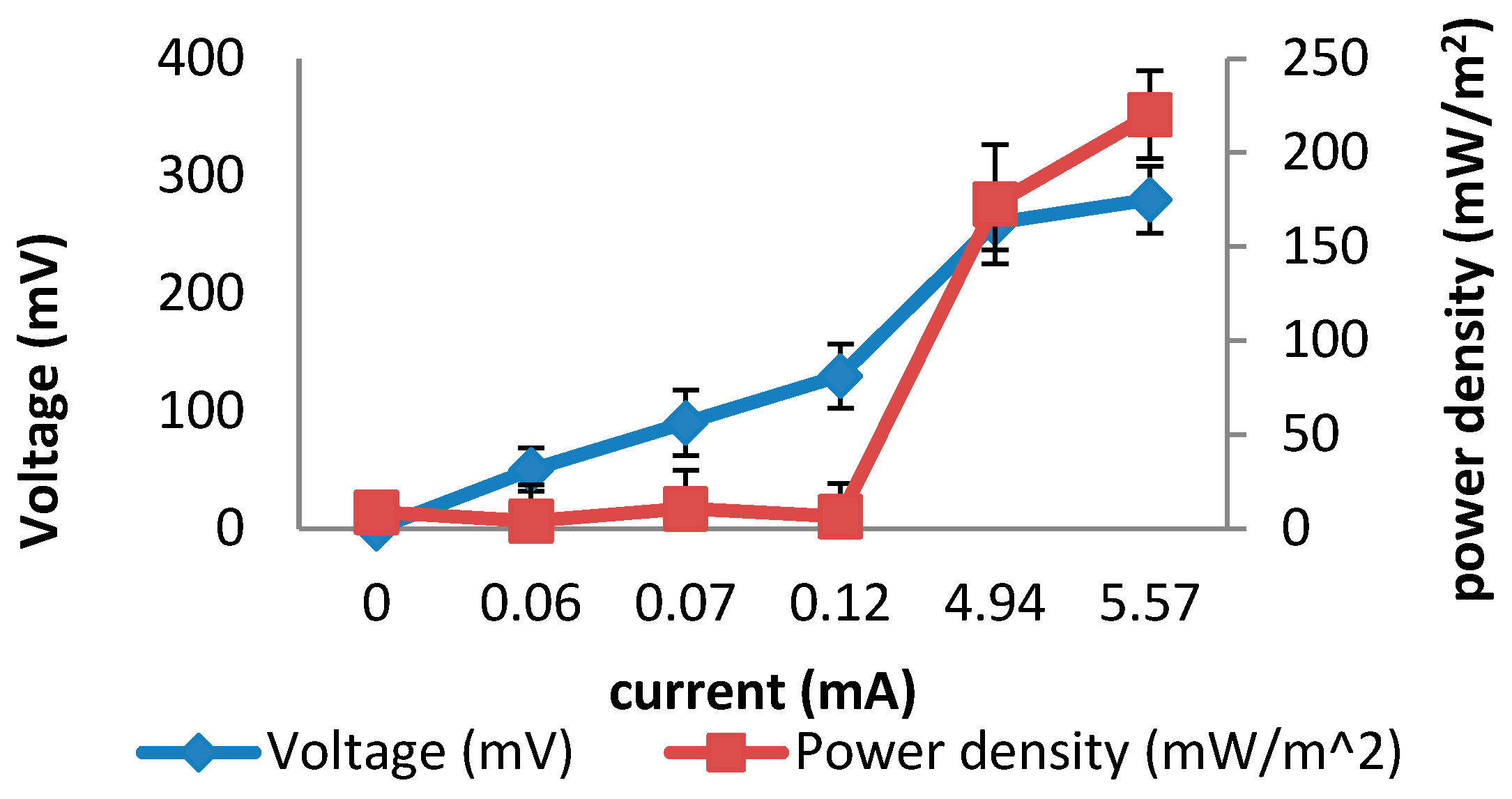
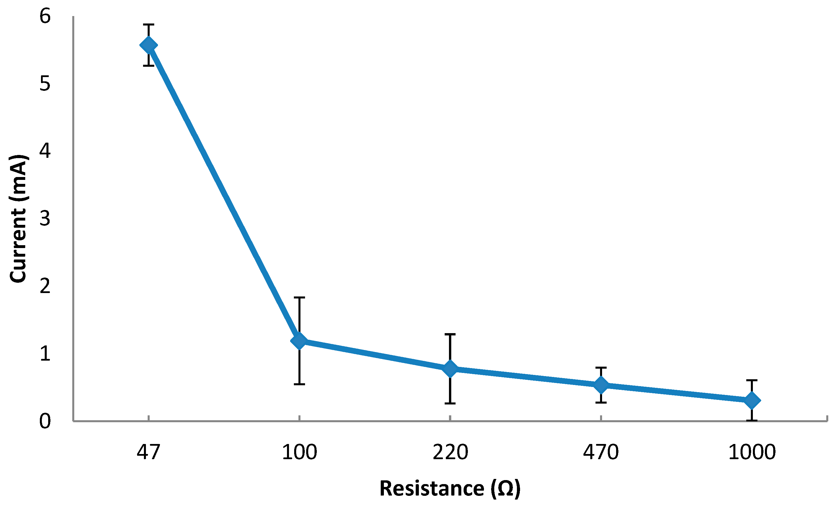
2.3.3. Performance of ML-MFC
3. Methodology
3.1. Sample Characterization
3.2. Analytical Methods
3.2.1. Elemental Analysis
3.2.2. Atomic Absorption Spectrometry (AAS)
3.2.3. Inductively Coupled Plasma Optical Emission Spectrometry (ICP-OES)
3.2.4. Determination of Biomass
3.2.5. Determination of Chemical Oxygen Demand (COD)
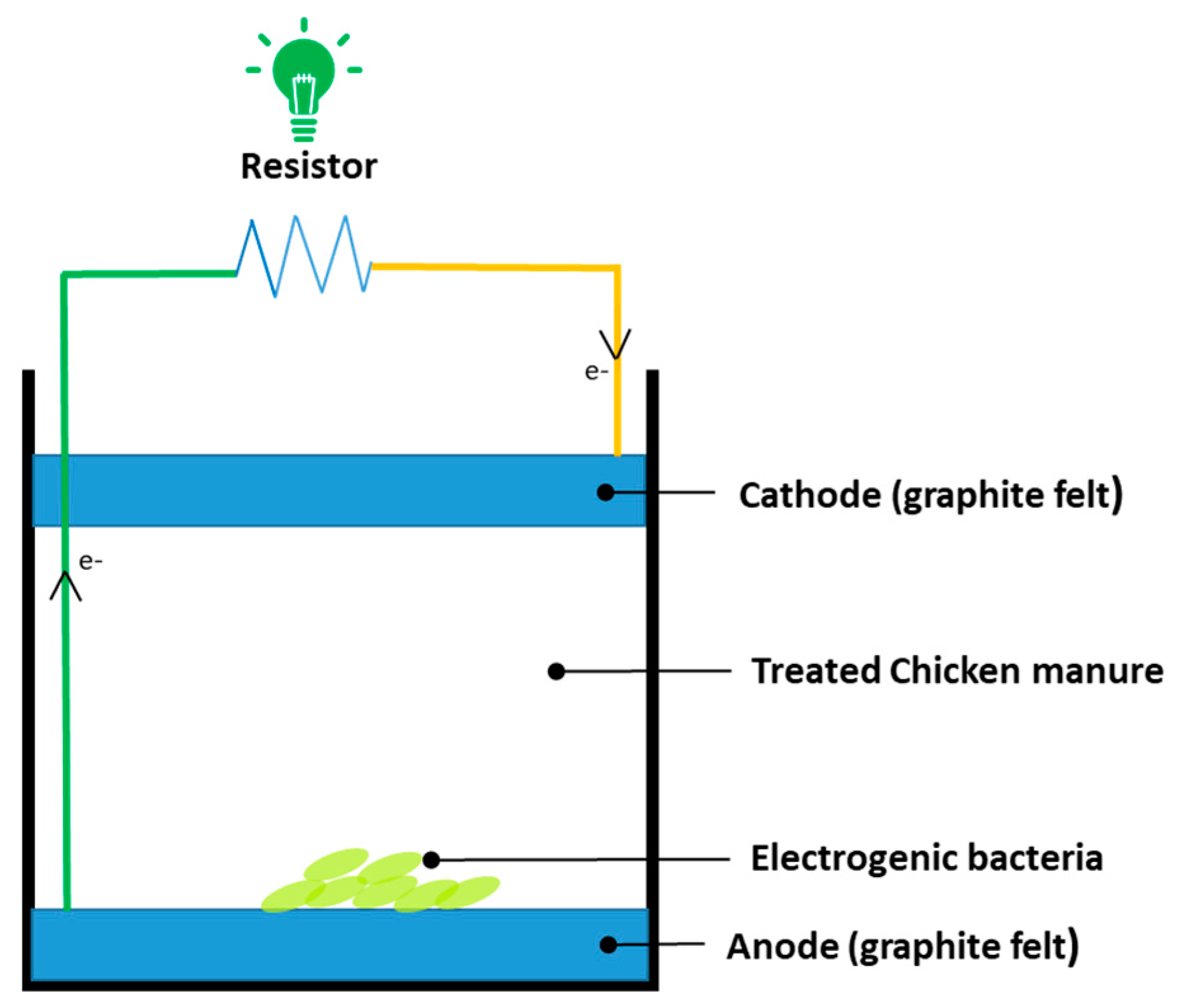
3.3. Configuration of ML-MFC
3.4. Statistical Experimental Design
Optimization Using Response Surface Methodology with Central Composite Design (CCD)
3.5. Determination of Power Using Polarization Curve
3.6. Operation of ML-MFC
3.7. Pretreatment of Chicken Manure
3.7.1. Thermal Pretreatment
3.7.2. Sonication Pretreatment
3.7.3. Alkaline Pretreatment
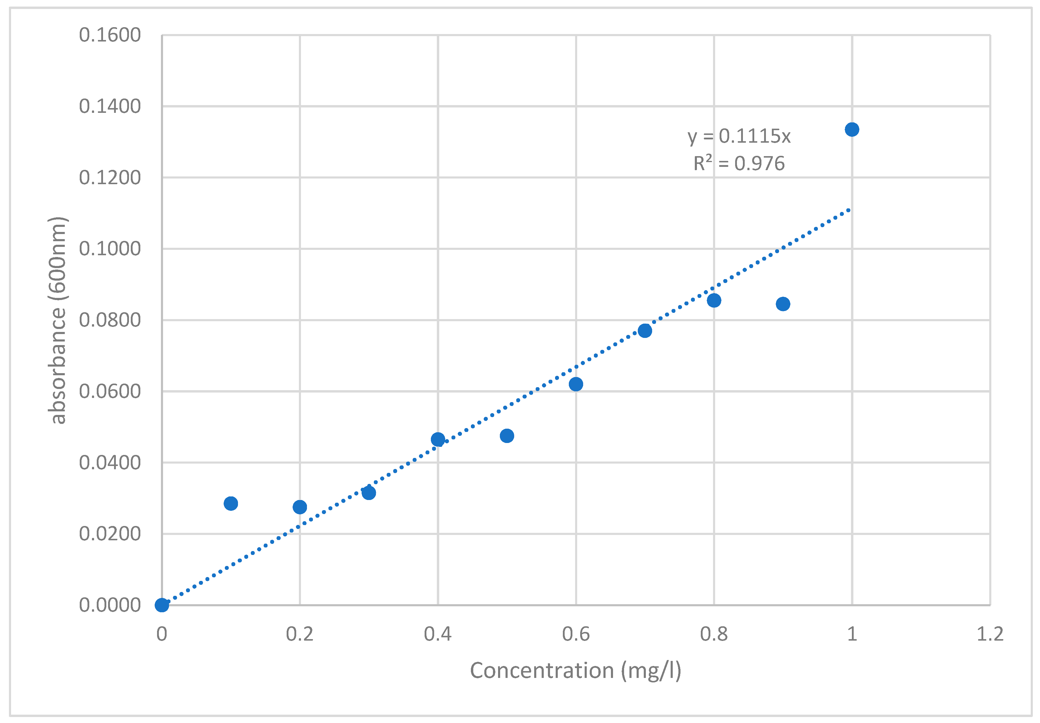
3.8. Preparation of Standard Calibration Curve
3.9. Growth Profile of Bacillus Subtillis
3.9.1. Preparation and Fermentation of Raw Broth from Chicken Manure
3.9.2. Specific Growth Rate of Electrogenic Bacteria
3.9.3. Doubling Time of Electrogenic Bacteria
4. Conclusions
Author Contributions
Funding
Data Availability Statement
Acknowledgments
Conflicts of Interest
Appendix A

References
- IEA. Global Energy Review 2020: The Impacts of the COVID-19 Crisis on Global Energy Demand and CO2 Emissions; OECD Publishing: Paris, France, 2020. [Google Scholar] [CrossRef]
- Yaqoob, A.A.; Khatoon, A.; Mohd Setapar, S.H.; Umar, K.; Parveen, T.; Mohamad Ibrahim, M.N.; Ahmad, A.; Rafatullah, M. Outlook on the role of microbial fuel cells in remediation of environmental pollutants with electricity generation. Catalysts 2020, 10, 819. [Google Scholar] [CrossRef]
- Abbas, S.Z.; Rafatullah, M.; Ismail, N.; Syakir, M.I. A review on sediment microbial fuel cells as a new source of sustainable energy and heavy metal remediation: Mechanisms and future prospective. Int. J. Energy Res. 2017, 41, 1242–1264. [Google Scholar] [CrossRef]
- Kusch-Brandt, S. Urban Renewable Energy on the Upswing: A Spotlight on Renewable Energy in Cities in REN21’s “Renewables 2019 Global Status Report”. Resources 2019, 8, 139. [Google Scholar] [CrossRef] [Green Version]
- Abbas, S.Z.; Rafatullah, M.; Ismail, N.; Nastro, R.A. Enhanced bioremediation of toxic metals and harvesting electricity through sediment microbial fuel cell. Int. J. Energy Res. 2017, 41, 2345–2355. [Google Scholar] [CrossRef]
- Abbas, S.Z.; Rafatullah, M.; Khan, M.A.; Siddiqui, M.R. Bioremediation and Electricity Generation by Using Open and Closed Sediment Microbial Fuel Cells. Front. Microbiol. 2019, 14, 3348. [Google Scholar] [CrossRef] [Green Version]
- Abbas, S.Z.; Rafatullah, M.; Ismail, N.; Shakoori, F.R. Electrochemistry and microbiology of microbial fuel cells treating marine sediments polluted with heavy metals. RSC Adv. 2018, 8, 18800–18813. [Google Scholar] [CrossRef] [Green Version]
- Orlando, M.Q.; Borja, V.M. Pretreatment of animal manure biomass to improve biogas production: A review. Energies 2020, 13, 3573. [Google Scholar] [CrossRef]
- Moradian, J.M.; Fang, Z.; Yong, Y.C. Recent advances on biomass-fueled microbial fuel cell. Bioresour. Bioprocess. 2021, 8, 14. [Google Scholar] [CrossRef]
- Hassan, S.H.A.; Gad El-Rab, S.M.F.; Rahimnejad, M.; Ghasemi, M.; Joo, J.-H.; Sik-Ok, Y.; Kim, I.S.; Oh, S.-E. Electricity generation from rice straw using a microbial fuel cell. Int. J. Hydrogen Energy 2014, 39, 9490–9496. [Google Scholar] [CrossRef]
- Tao, K.; Quan, X.; Quan, Y. Composite vegetable degradation and electricity generation in microbial fuel cell with ultrasonic pretreatment. Environ. Eng. Manag. J. 2013, 12, 1423–1427. [Google Scholar] [CrossRef]
- Ong, T.; Hou, S.; Zhang, J.; Wang, H.; Xie, J. Production of Electricity from Rice Straw with different Pretreatment Methods Using a Sediment Microbial Fuel Cell. Int. J. Electrochem. Sci. 2018, 13, 461–471. [Google Scholar]
- Liu, H.; Cheng, S.; Logan, B.E. Production of Electricity from Acetate or Butyrate Using a Single-Chamber Microbial Fuel Cell. Environ. Sci. Technol. 2005, 39, 658–662. [Google Scholar] [CrossRef] [PubMed]
- Pant, D.; Van Bogaert, G.; Diels, L.; Vanbroekhoven, K. A review of the substrates used in microbial fuel cells (MFCs) for sustainable energy production. Bioresour. Technol. 2010, 101, 1533–1543. [Google Scholar] [CrossRef]
- Hu, Z. Electricity generation by a baffle-chamber membraneless microbial fuel cell. J. Power Sources 2008, 179, 27–33. [Google Scholar] [CrossRef]
- Park, Y.; Cho, H.; Yu, J.; Min, B.; Kim, H.S.; Kim, B.G. Response of microbial community structure to pre-acclimation strategies in microbial fuel cells for domestic wastewater treatment. Bioresour. Technol. 2017, 233, 176–183. [Google Scholar] [CrossRef]
- Rezaei, F.; Richard, T.L.; Logan, B.E. Enzymatic hydrolysis of cellulose coupled with electricity generation in a microbial fuel cell. Biotechnol. Bioeng. 2008, 101, 1163–1169. [Google Scholar] [CrossRef] [PubMed]
- Sangcharoen, A.; Niyom, W.; Suwannasilp, B.B. A microbial fuel cell treating organic wastewater containing high sulfate under continuous operation: Performance and microbial community. Process Biochem. 2015, 50, 1648–1655. [Google Scholar] [CrossRef]
- Wang, Y.-Z.; Shen, Y.; Gao, L.; Liao, Z.-H.; Sun, J.-Z.; Yong, Y.-C. Improving the extracellular electron transfer of Shewanella oneidensis MR-1 for enhanced bioelectricity production from biomass hydrolysate. RSC Adv. 2017, 7, 30488–30494. [Google Scholar] [CrossRef] [Green Version]
- Pandit, S.; Savla, N.; Sonawane, J.M.; Muh, A.; Gupta, P.K.; Prasad, R. Agricultural Waste and Wastewater as Feedstock for Bioelectricity Generation Using Microbial Fuel Cells: Recent Advances. Fermentation 2021, 7, 169. [Google Scholar] [CrossRef]
- Umar, M.F.; Rafatullah, M.; Abbas, S.Z.; Ibrahim, M.N.M.; Ismail, N. Bioelectricity production and xylene biodegradation through double chamber benthic microbial fuel cells fed with sugarcane waste as a substrate. J. Hazard. Mater. 2021, 419, 126469. [Google Scholar] [CrossRef]
- Umar, M.F.; Rafatullah, M.; Abbas, S.Z.; Ibrahim, M.N.M.; Ismail, N. Enhanced benzene bioremediation and power generation by double chamber benthic microbial fuel cells fed with sugarcane waste as a substrate. J. Clean. Prod. 2021, 310, 127583. [Google Scholar] [CrossRef]
- Uçkun, E.; Trzcinski, A.P.; Jern, W.; Liu, Y. Bioconversion of food waste to energy: A review. Fuel 2014, 134, 389–399. [Google Scholar] [CrossRef]
- Moqsud, M.A.; Omine, K.; Yasufuku, N.; Bushra, Q.S.; Hyodo, M.; Nakata, Y. Bioelectricity from kitchen and bamboo waste in a microbial fuel cell. Waste Manag. Res. 2014, 32, 124–130. [Google Scholar] [CrossRef] [PubMed]
- Khater, D.; Hazaa, M.; Hassan, R.Y.A. Activated Sludge-based Microbial Fuel Cell for Bio-electricity Generation. J. Basic Environ. Sci. 2015, 2, 63–72. [Google Scholar]
- Fantozzi, F.; D’Alessandro, B.; Leonardi, D.; Desideri, U. Evaluation of available technologies for chicken manure energy conversion and techno-economic assessment of a case study in Italy. Proc. ASME Turbo Expo 2004, 7, 647–655. [Google Scholar]
- Ermis, H.; Guven-Gulhan, U.; Cakir, T.; Altinbas, M. Effect of iron and magnesium addition on population dynamics and high value product of microalgae grown in anaerobic liquid digestate. Sci. Rep. 2020, 10, 1–12. [Google Scholar]
- Merchant, S.S.; Helmann, J.D. Elemental Economy. Microbial Strategies for Optimizing Growth in the Face of Nutrient Limitation. Adv. Microb. Physiol. 2012, 60, 91–210. [Google Scholar] [CrossRef] [Green Version]
- Zhang, C.; Li, W.; Hu, M.; Cheng, X.; He, K.; Mao, L. A Comparative Study of Using Polarization Curve Models in Proton Exchange Membrane Fuel Cell Degradation Analysis. Energies 2020, 13, 3759. [Google Scholar] [CrossRef]
- Jiang, H.; Ali, M.A.; Xu, Z.; Halverson, L.J.; Dong, L. Integrated Microfluidic Flow-Through Microbial Fuel Cells. Sci. Rep. 2017, 7, 41208. [Google Scholar] [CrossRef] [Green Version]
- Turek, A.; Wieczorek, K.; Wolf, W.M. Digestion procedure and determination of heavy metals in sewage sludge-an analytical problem. Sustainability 2019, 11, 1753. [Google Scholar] [CrossRef] [Green Version]
- Heydarian, M.; Hajinorouzi, F.; Khosrowzadeh, A.; Beheshti, S.I.; Emami, M. Insight into the provenance and clustering of Middle Chalcolithic Ceramics from Chaharmahal-Bakhtiari, Iran: Using petrographic and ICP-OES analysis. J. Archaeol. Sci. Rep. 2020, 34, 102655. [Google Scholar] [CrossRef]
- Karpiuk, U.V.; Al Azzam, K.M.; Abudayeh, Z.H.M.; Kislichenko, V.; Naddaf, A.; Cholak, I.; Yemelianova, O. Qualitative and quantitative content determination of macro-minor elements in Bryonia alba l. roots using flame atomic absorption spectroscopy technique. Adv. Pharm. Bull. 2016, 6, 285–291. [Google Scholar] [CrossRef] [PubMed]
- Muaz, M.Z.M.; Abdul, R.; Vadivelu, V.M. Recovery of energy and simultaneous treatment of dewatered sludge using membrane-less microbial fuel cell. Environ. Prog. Sustain. Energy 2019, 38, 208–219. [Google Scholar] [CrossRef] [Green Version]
- Nwaigwe, K.N.; Enweremadu, C.C. Analysis of Chemical Oxygen Demand (COD) Removal Rate Using Upflow Bioreactor with Central Substrate Dispenser (UBCSD). In Proceedings of the 4th International Conference on Advances in Engineering Sciences and Applied Mathematics, Kuala Lumpur, Malaysia, 8–9 December 2015; pp. 67–70. [Google Scholar]
- Logan, B.E.; Hamelers, B.; Rozendal, R.; Schröder, U.; Keller, J.; Freguia, S.; Aelterman, P.; Verstraete, W.; Rabaey, K. Microbial fuel cells: Methodology and technology. Environ. Sci. Technol. 2006, 40, 5181–5192. [Google Scholar] [CrossRef] [PubMed]
- Tranter, J.; Crawford, K.; Richardson, J.; Schollar, J. Basic Practical Microbiology. Basic Pract. Microbiol. 2016, 46. [Google Scholar]
- Smith, R.H. Plant Tissue Culture; Elsevier: Amsterdam, The Netherlands, 2013. [Google Scholar]


| Types | Element | Unit | Untreated Chicken Manure | Treated Chicken Manure |
|---|---|---|---|---|
| Macronutrient | Carbon (C) | % | 34.20 | 35.12 |
| Hydrogen (H) | % | 2.86 | 3.18 | |
| Nitrogen (N) | % | 4.05 | 4.16 | |
| Micronutrient | Magnesium (Mg) | mg/L | 71.61 | 78.03 |
| Iron (Fe) | mg/L | 9.7 | 10.5 | |
| Trace element | Zinc (Zn) | mg/L | 4.6 | 3.9 |
| Manganese (Mn) | mg/L | 5.4 | 6.3 | |
| Cadmium (Cd) | mg/L | 1.7 | 2.2 | |
| Organic carbon | mg/L | 517 | 610 |
| Run | Variables a | Response 1 COD Removal Efficiency (%) | Response 2 Biomass (mg/L) | Response 3 Power Density (mW/m2) | ||
|---|---|---|---|---|---|---|
| A | B | C | ||||
| °C | kHz | pH | ||||
| 1 | −1 | 0 | −1 | 30.4 | 6.521 | 77.25 |
| 2 | +1 | 0 | −1 | 43.855 | 6.723 | 93.241 |
| 3 | −1 | +1 | −1 | 35.12 | 6.608 | 89.168 |
| 4 | +1 | +1 | −1 | 48.21 | 6.689 | 95.32 |
| 5 | −1 | 0 | +1 | 79.548 | 7.402 | 168.66 |
| 6 | +1 | 0 | +1 | 81.025 | 6.780 | 160.41 |
| 7 | −1 | +1 | +1 | 76.124 | 6.833 | 173.48 |
| 8 | +1 | +1 | +1 | 74.891 | 6.608 | 186.34 |
| 9 | −1 | 0 | 0 | 64.194 | 6.724 | 120.6 |
| 10 | +1 | 0 | 0 | 98.305 | 7.698 | 205.228 |
| 11 | 0 | −1 | 0 | 86.546 | 7.690 | 118.195 |
| 12 | 0 | +1 | 0 | 89.618 | 6.807 | 62.842 |
| 13 | 0 | 0 | −1 | 81.320 | 6.834 | 85.566 |
| 14 | 0 | 0 | +1 | 87.213 | 7.03 | 200.14 |
| 15 | 0 | 0 | 0 | 72.412 | 7.256 | 211.02 |
| 16 | 0 | 0 | 0 | 84.745 | 7.02 | 180.3 |
| 17 | 0 | 0 | 0 | 79.731 | 7.381 | 194.3 |
| 18 | 0 | 0 | 0 | 83.792 | 7.156 | 195.7 |
| 19 | 0 | 0 | 0 | 80.685 | 7.853 | 220.089 |
| 20 | 0 | 0 | 0 | 80.658 | 7.831 | 220.089 |
| Responds | Source | Sum of Squares | df | Mean Square | F-Value | p-Value |
|---|---|---|---|---|---|---|
| COD removal efficiency (%) | Linear | 1461.69 | 3 | 487.23 | 0.6569 | 0.5904 |
| 2FI | 2355.60 | 3 | 785.20 | 1.07 | 0.3945 | |
| Quadratic | 3831.79 | 3 | 1277.26 | 2.25 | 0.0325 | |
| Cubic | 1905.01 | 4 | 476.25 | 0.7569 | 0.5890 | |
| Biomass (mg/L) | Linear | 0.1228 | 3 | 0.0409 | 1.13 | 0.3682 |
| 2FI | 0.0335 | 3 | 0.0112 | 0.265 | 0.8493 | |
| Quadratic | 0.3179 | 3 | 0.1060 | 4.60 | 0.0285 | |
| Cubic | 0.0959 | 4 | 0.0240 | 1.07 | 0.4464 | |
| Power density (mW/m2) | Linear | 40,798.46 | 3 | 13,599.49 | 3.01 | 0.0612 |
| 2FI | 9376.89 | 3 | 3125.63 | 0.645 | 0.5997 | |
| Quadratic | 15,037.17 | 3 | 5012.39 | 1.05 | 0.0381 | |
| Cubic | 20,691.97 | 4 | 5172.99 | 1.14 | 0.4215 |
| Source | Sum of Squares | df | Mean Square | F-Value | p-Value | |
|---|---|---|---|---|---|---|
| COD removal efficiency (%) | Linear | 11,438.60 | 11 | 1039.87 | 12.11 | 0.0015 |
| 2FI | 9083.00 | 8 | 1135.37 | 13.23 | 0.0009 | |
| Quadratic | 5251.21 | 5 | 1050.24 | 12.23 | 0.2681 | |
| Cubic | 3346.20 | 1 | 3346.20 | 38.98 | 0.0002 | |
| Pure error | 429.24 | 5 | 85.85 | |||
| Biomass (mg/L) | Linear | 0.4881 | 11 | 0.0444 | 2.37 | 0.1755 |
| 2FI | 0.4546 | 8 | 0.0568 | 3.04 | 0.1181 | |
| Quadratic | 0.1367 | 5 | 0.0273 | 1.46 | 0.3435 | |
| Cubic | 0.0408 | 1 | 0.0408 | 2.18 | 0.1999 | |
| Pure error | 0.0935 | 5 | 0.0187 | |||
| Power density (mW/m2) | Linear | 45,749.87 | 11 | 4159.08 | 0.7815 | 0.6606 |
| 2FI | 36,372.98 | 8 | 4546.62 | 0.8543 | 0.5995 | |
| Quadratic | 21,335.81 | 5 | 4267.16 | 0.8018 | 0.5928 | |
| Cubic | 643.84 | 1 | 643.84 | 0.1210 | 0.7421 | |
| Pure error | 26,609.24 | 5 | 5321.85 |
| Respond | Source | Sum of Square | df | Mean Square | F-Value | p-Value |
|---|---|---|---|---|---|---|
| COD removal efficiency | Model | 7649.08 | 9 | 849.90 | 1.50 | 0.0171 |
| A—thermal | 804.16 | 1 | 804.16 | 1.42 | 0.0186 | |
| B—sonication | 139.64 | 1 | 139.64 | 0.2458 | 0.0201 | |
| C—alkaline | 1063.64 | 1 | 1063.64 | 1.87 | 0.0194 | |
| AB | 221.96 | 1 | 221.96 | 0.3908 | 0.0215 | |
| AC | 1273.80 | 1 | 1273.80 | 2.24 | 0.0369 | |
| BC | 859.83 | 1 | 859.83 | 1.51 | 0.0281 | |
| A² | 304.07 | 1 | 304.07 | 0.5353 | 0.4812 | |
| B² | 40.40 | 1 | 40.40 | 0.0711 | 0.7951 | |
| C² | 3473.47 | 1 | 3473.47 | 6.11 | 0.0329 | |
| Lack of fit | 5251.21 | 5 | 1050.24 | 12.23 | 0.5271 | |
| R2 | 0.8917 |
| Respond | Source | Sum of Square | df | Mean Square | F-Value | p-Value |
|---|---|---|---|---|---|---|
| Biomass (mg/L) | Model | 0.4742 | 9 | 0.0527 | 2.29 | 0.0265 |
| A—thermal | 0.0587 | 1 | 0.0587 | 2.55 | 0.0175 | |
| B—sonication | 0.0642 | 1 | 0.0642 | 2.79 | 0.0249 | |
| C—alkaline | 0.0010 | 1 | 0.0010 | 0.044 | 0.0146 | |
| AB | 0.0022 | 1 | 0.0022 | 0.097 | 0.0134 | |
| AC | 0.0101 | 1 | 0.0101 | 0.440 | 0.0352 | |
| BC | 0.0212 | 1 | 0.0212 | 0.919 | 0.0371 | |
| A² | 0.1587 | 1 | 0.1587 | 6.90 | 0.0253 | |
| B² | 0.0539 | 1 | 0.0539 | 2.34 | 0.1571 | |
| C² | 0.0768 | 1 | 0.0768 | 3.34 | 0.0978 | |
| Lack of fit | 0.1367 | 5 | 0.0273 | 1.46 | 0.3435 | |
| R2 | 0.9101 |
| Respond | Source | Sum of Square | df | Mean Square | F-Value | p-Value |
|---|---|---|---|---|---|---|
| Power density (mW/m2) | Model | 65,212.51 | 9 | 7245.83 | 1.51 | 0.0421 |
| A—thermal | 25,964.81 | 1 | 25,964.81 | 5.42 | 0.0310 | |
| B—sonication | 1826.47 | 1 | 1826.47 | 0.381 | 0.0408 | |
| C—alkaline | 3265.08 | 1 | 3265.08 | 0.681 | 0.0344 | |
| AB | 6091.25 | 1 | 6091.25 | 1.27 | 0.2860 | |
| AC | 3188.00 | 1 | 3188.00 | 0.664 | 0.4338 | |
| BC | 97.64 | 1 | 97.64 | 0.020 | 0.8894 | |
| A² | 618.93 | 1 | 618.93 | 0.129 | 0.7268 | |
| B² | 5176.80 | 1 | 5176.80 | 1.08 | 0.3232 | |
| C² | 11,755.23 | 1 | 11,755.23 | 2.45 | 0.1485 | |
| Lack of fit | 21,335.81 | 5 | 4267.16 | 0.801 | 0.5928 | |
| R2 | 0.8794 |
| Parameters | Unit | Value |
|---|---|---|
| Sonication | kHz | 20.8916 |
| Thermal | °C | 140.632 |
| Alkaline | pH | 11.0583 |
| Response 1—biomass | mg/L | 7.34048 |
| Response 2—COD removal | % | 86.192 |
| Response 3—power density | mW/m2 | 207.108 |
| Desirability | 1.000 |
| COD Removal | Biomass | Power Density | |||||||
|---|---|---|---|---|---|---|---|---|---|
| No. | Exp. | Pred. | ε | Exp. | Pred. | ε | Exp. | Pred. | ε |
| 1 | 82.002 | 86.19 | −5.19 | 7.102 | 7.340 | −0.23 | 198.400 | 207.10 | −8.70 |
| 2 | 84.874 | 86.19 | −1.31 | 7.119 | 7.340 | −0.22 | 202.100 | 207.10 | −5.00 |
| 3 | 87.300 | 86.19 | 1.108 | 7.404 | 7.340 | 0.063 | 209.970 | 207.10 | 2.862 |
| 4 | 89.351 | 86.19 | 3.159 | 7.588 | 7.340 | 0.248 | 211.471 | 207.10 | 4.363 |
| 5 | 90.062 | 86.19 | 3.870 | 7.542 | 7.340 | 0.202 | 213.620 | 207.10 | 6.512 |
| Mean | 86.7178 | 86.192 | 0.3258 | 7.35142 | 7.34048 | 0.01094 | 207.1122 | 207.108 | 0.0042 |
| SD | 3.320 | 0.230 | 6.529 | ||||||
| 95%cl | 81.8824–90.5016 | 6.973456–7.707504 | 196.7526–217.4634 | ||||||
| Condition | Doubling Time, Td | Specific Growth Rate µ |
|---|---|---|
| Untreated chicken manure | 6.08 h | 0.11 h−1 |
| Treated chicken manure | 3.43 h | 0.20 h−1 |
| Coded Variables Level | ||||
|---|---|---|---|---|
| Low | Centre | High | ||
| Factor | Variables | −1 | 0 | +1 |
| A | Thermal pretreatment (°C) | 135 | 140 | 145 |
| B | Sonication pretreatment (kHz) | 15 | 20 | 25 |
| C | Alkaline pretreatment (pH) | 8 | 10 | 12 |
Publisher’s Note: MDPI stays neutral with regard to jurisdictional claims in published maps and institutional affiliations. |
© 2022 by the authors. Licensee MDPI, Basel, Switzerland. This article is an open access article distributed under the terms and conditions of the Creative Commons Attribution (CC BY) license (https://creativecommons.org/licenses/by/4.0/).
Share and Cite
Mohd Azmi, N.; Mohd Sabri, M.N.I.; Tajarudin, H.A.; Shoparwe, N.F.; Makhtar, M.M.Z.; Shukor, H.; Alam, M.; Siddiqui, M.R.; Rafatullah, M. The Effect of Different Pretreatment of Chicken Manure for Electricity Generation in Membrane-Less Microbial Fuel Cell. Catalysts 2022, 12, 810. https://0-doi-org.brum.beds.ac.uk/10.3390/catal12080810
Mohd Azmi N, Mohd Sabri MNI, Tajarudin HA, Shoparwe NF, Makhtar MMZ, Shukor H, Alam M, Siddiqui MR, Rafatullah M. The Effect of Different Pretreatment of Chicken Manure for Electricity Generation in Membrane-Less Microbial Fuel Cell. Catalysts. 2022; 12(8):810. https://0-doi-org.brum.beds.ac.uk/10.3390/catal12080810
Chicago/Turabian StyleMohd Azmi, Nurhazirah, Muhammad Najib Ikmal Mohd Sabri, Husnul Azan Tajarudin, Noor Fazliani Shoparwe, Muaz Mohd Zaini Makhtar, Hafiza Shukor, Mahboob Alam, Masoom Raza Siddiqui, and Mohd Rafatullah. 2022. "The Effect of Different Pretreatment of Chicken Manure for Electricity Generation in Membrane-Less Microbial Fuel Cell" Catalysts 12, no. 8: 810. https://0-doi-org.brum.beds.ac.uk/10.3390/catal12080810