Artificial Intelligence Modelling Approach for the Prediction of CO-Rich Hydrogen Production Rate from Methane Dry Reforming

Abstract

This study investigates the applicability of the Leven–Marquardt algorithm, Bayesian regularization, and a scaled conjugate gradient algorithm as training algorithms for an artificial neural network (ANN) predictively modeling the rate of CO and H₂ production by methane dry reforming over a Co/Pr₂O₃ catalyst. The dataset employed for the ANN modeling was obtained using a central composite experimental design. The input parameters consisted of CH₄ partial pressure, CO₂ partial pressure, and reaction temperature, while the target parameters included the rate of CO and H₂ production. A neural network architecture of 3 13 2, 3 15 2, and 3 15 2 representing the input layer, hidden neuron layer, and target (output) layer were employed for the Leven–Marquardt, Bayesian regularization, and scaled conjugate gradient training algorithms, respectively. The ANN training with each of the algorithms resulted in an accurate prediction of the rate of CO and H₂ production. The best prediction was, however, obtained using the Bayesian regularization algorithm with the lowest standard error of estimates (SEE). The high values of coefficient of determination (R² > 0.9) obtained from the parity plots are an indication that the predicted rates of CO and H₂ production were strongly correlated with the observed values.

1. Introduction

Methane dry reforming is a thermo-catalytic process used for producing synthetic gas (syngas), a mixture of hydrogen (H₂) and carbon monoxide (CO), by utilizing methane (CH₄) and carbon dioxide (CO₂) as feedstocks [1]. Although there are several processes such as steam methane reforming [2], coal gasification [3], glycerol reforming [4], and partial oxidation reforming [5] that can be employed for syngas production, none of these processes have the advantages of mitigating greenhouse gas emission through the consumption of CH₄ and CO₂ [6]. Besides being a potential technical route for greenhouse gas emission reduction, methane dry reforming has the advantage of producing syngas with a H₂:CO ratio close to unity [7]. The syngas produced can in turn be used as an important building block for many industrial processes such as ammonia, methanol, and synthetic fuel production [8]. However, one of the key challenges of the methane dry reforming process is catalyst deactivation by carbon deposition and sintering which is caused due to the high temperature (>873 K) required for the reaction [9].

To overcome these challenges, several supported metal-based catalysts have been developed and tested. An extensive review by Abdullah et al. [10] revealed that supported nickel (Ni) catalysts have been mostly investigated for methane dry reforming due to its high catalytic performance. Nevertheless, the Ni-based catalysts are very prone to sintering and carbon deposition [11]. On the other hand, cobalt (Co)-based catalysts which have a comparative activity to Ni have been reported to show superior stability compare to Ni under the same process condition [12,13]. In our previous studies, the use of rare-earth metal oxide-supported Co catalysts for CO-rich hydrogen production showed considerable activity and stability [14,15,16]. However, one major challenge is understanding the kinetics of the methane dry reforming in terms of the rate of H₂ and CO production due to variations in the chemical composition of the various catalysts [17]. This challenge can be overcome by employing an artificial intelligence modeling approach for a better understanding of the process parameters [18,19]. Processes with non-linear and complex relationships between the input and the output parameters are often encountered in real life processes. The better understanding of the non-linear relationship between the input and the output parameters of the process can further be utilized to optimize the process operation and create the basis for the theoretical framework, process automation, and upscaling [20].

An artificial intelligence modeling approach using an artificial neural network (ANN) has been widely employed for different catalytic processes, such as hydrodesulfurization [20], methanol steam reforming, glycerol steam reforming [21,22], air gasification of biomass [23], water gas shift reaction [24], and steam gasification of palm oil waste [25]. Nasr et al. [26] reported the use of ANN for the predictive modeling of biohydrogen production using a back-propagation configuration and concluded that the experimental and the predicted biohydrogen production were strongly correlated. Zamaniyan et al. [27] employed a three-layer back-propagation feed-forward ANN for modeling industrial plant hydrogen. The study revealed that the ANN accurately predicted the temperature, pressure, and mole fraction of the hydrogen production in the plant. Ghasemzadeh et al. [28] predicted the performance of a silica membrane reactor during methanol steam reforming using a multilayer perceptron ANN. The study shows that the membrane pressure, temperature, and gas hourly space velocity were accurately predicted with a strong correlation between the actual and the predicted values. In a similar study by Ghasemzadeh et al. [22], ANN was also employed for the predictive modeling of hydrogen production by glycerol steam reforming over a Co/Al₂O₃ catalyst. The feed forward ANN accurately predicted the glycerol conversion, H₂ recovery, H₂ yield, H₂ selectivity, CO selectivity, and CO₂ selectivity with a high coefficient of determination (R²) and low mean square error (MSE). In our previous study, ANN has been employed for the prediction of CH₄ conversion, CO₂ conversion, and syngas ratio from methane dry reforming over Sm₂O₃- and CeO₂- supported Co catalysts [19]. In all the above studies, the Leven–Marquardt algorithm was employed for the training of the ANN. In this study, the effect of employing three training algorithms, namely Leven–Marquardt, Bayesian regulation, and scaled conjugate gradient, on the predictability of the ANN model was investigated. The effectiveness of each of the trained ANN configurations was tested through the predicted rate of H₂ and CO production from the Co/Pr₂O₃-catalyzed methane dry reforming process.

2. Results and Discussions

2.1. Generated Data for the ANN Modeling

The data obtained from the experimental runs using a central composite design (CCD) are summarized in

Table 1. Data obtained from central composite experimental design for artificial neural network (ANN) modeling.

S/N	Reaction Temperature (K)	CH4 Partial Pressure (kPa)	CO2 Partial Pressure (kPa)	Rate of CO Production (mmol/gcat/min)	Rate of H2 Production (mmol/gcat/min)
1	973	27.5	27.5	0.2880	0.1032
2	1023	15.0	40.0	0.3085	0.1103
3	973	27.5	48.5	0.1736	0.0918
4	973	27.5	27.5	0.2878	0.1030
5	973	27.5	27.5	0.2879	0.1029
6	973	27.5	27.5	0.2878	0.1030
7	973	6.5	27.5	0.0013	0.0078
8	973	27.5	27.5	0.2881	0.1029
9	973	27.5	27.5	0.2878	0.1030
10	973	27.5	27.5	0.2879	0.1031
11	973	27.5	27.5	0.2881	0.1028
12	973	27.5	27.5	0.2880	0.1030
13	1023	40.0	15.0	0.3577	0.2601
14	973	27.5	27.5	0.2882	0.1031
15	923	40.0	40.0	0.0938	0.0422
16	1057	27.5	27.5	0.4623	0.3471
17	973	27.5	27.5	0.2878	0.1029
18	973	27.5	27.5	0.2880	0.1030
19	973	27.5	27.5	0.2881	0.1031
20	973	27.5	27.5	0.2879	0.1029
21	973	27.5	27.5	0.2878	0.1029
22	923	15.0	40.0	0.0381	0.0002
23	973	27.5	27.5	0.2877	0.1031
24	973	27.5	27.5	0.2880	0.1030
25	973	27.5	27.5	0.2876	0.1029
26	973	27.5	6.5	0.1581	0.0134
27	973	27.5	27.5	0.2874	0.1031
28	973	27.5	27.5	0.2877	0.1030
29	973	27.5	27.5	0.2880	0.1029
30	973	27.5	27.5	0.2878	0.1031
31	1023	15.0	15.0	0.3085	0.0113
32	973	27.5	27.5	0.2863	0.1029
33	1023	40.0	40.0	0.3624	0.2341
34	973	48.5	27.5	0.3495	0.1515
35	973	27.5	27.5	0.2878	0.1031
36	923	40.0	15.0	0.0728	0.0021
37	973	27.5	27.5	0.0877	0.013
38	973	27.5	27.5	0.0874	0.0129
39	923	15.0	15.0	0.0281	0.001
40	973	27.5	27.5	0.2881	0.1029
41	973	27.5	27.5	0.2880	0.1031
42	973	27.5	27.5	0.2878	0.1030
43	973	27.5	27.5	0.2880	0.1029
44	973	27.5	27.5	0.2879	0.1031
45	973	27.5	27.5	0.2878	0.1029
46	973	27.5	27.5	0.2880	0.1030
47	973	27.5	27.5	0.2881	0.1031
48	889	27.5	27.5	0.1379	0.0919
49	973	27.5	27.5	0.2880	0.1029
50	973	27.5	27.5	0.2878	0.1030

. The data consist of 50 experimental runs which are made up of treatment combinations of reaction temperature, CH₄ partial pressure, and CO₂ partial pressure as input parameters, while the target parameters include the rate of CO and H₂ production. The responses (target values) obtained from each of the experimental runs varies according to the treatment combinations of the reaction temperature, CH₄ partial pressure, and CO₂ partial pressure.

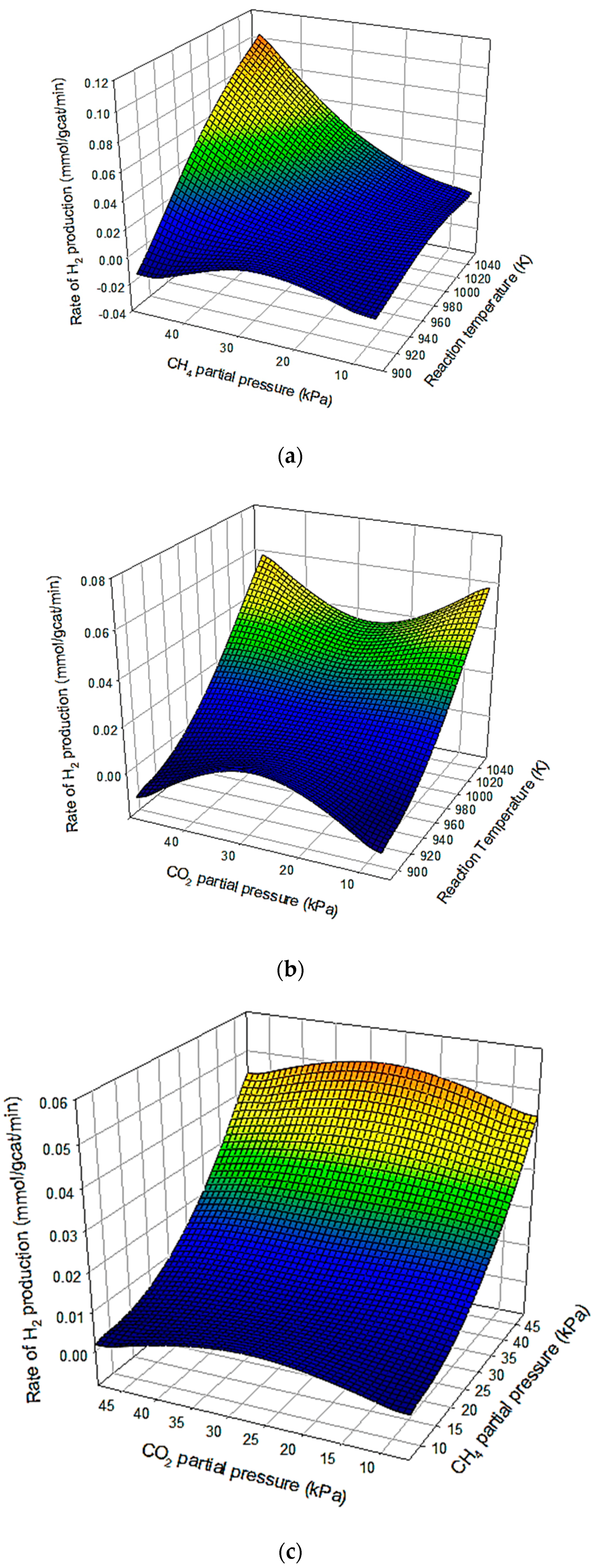
2.2. Interaction Effect of Process Parameters on the Rate of H₂ Production

Theoretically, a catalyzed methane dry reforming reaction as represented in Equation (1) involves the consumption of 1 mole of CH₄ and 1 mole CO₂ to produce 2 moles of CO and 2 moles of H₂ [29].

$${\mathrm{CH}}_4+{\mathrm{CO}}_2\rightleftharpoons 2\mathrm{CO}+2{\mathrm{H}}_2\Delta H_{298K}=+247\mathrm{kJ}/\mathrm{mol}$$

(1)

The methane dry reforming process is highly endothermic [30]. Therefore, the reaction is favored by a high temperature >900 K [31]. Although, the mechanism of the methane dry reforming reaction is strongly dependent on the nature of the catalyst, it is generally believed that the reaction commences with the activation of CH₄ and CO₂ being adsorbed on the catalyst active sites [32]. The activation of the adsorbed CH₄ often leads to the formation of carbon and hydrogen. While the activation of the CO₂ often occurs at the interphase of the catalyst active site and the support often leads to the formation of CO and surface O₂, which is simultaneously utilized to gasify the carbon formed during the activation of CH₄ [10]. The partial pressure of CH₄ and CO₂ at varying temperatures are crucial in determining the rate of production of CO and H₂ during the methane dry reforming process [32].

Figure 1a–c shows the interaction effect of the CH₄ partial pressure, CO₂ partial pressure, and reaction temperature on the rate of H₂ production. As shown in Figure 1a, the rate of H₂ production was significantly influenced by the CH₄ partial pressure and reaction temperature. The rate of H₂ production increased steadily with an increase in the CH₄ partial pressure until 30 kPa and thereafter decreased. This phenomenon can be attributed to the dominance of methane cracking whereby the CH₄ is activated on the catalyst active site to give H₂ and carbon. The carbon formed is often gasified by the release of surface O₂ through the activation of CO₂. In the case where the rate of gasification of the carbon is not at equilibrium with the release of the surface, there would be net carbon deposition which often results in catalyst deactivation. The deactivation of the catalyst active site by the deposited carbon could be responsible for the decrease in the rate of H₂ production at CH₄ partial pressure >30 kPa. At a low CH₄ partial pressure, the rate of H₂ production was low and steady due to a high concentration of CO₂ present in the reactant mixture. However, as the CH₄ partial pressure increased to measure up with that of CO₂, an increase in the rate of H₂ was observed which is typical for the methane dry reforming reaction [33]. Similarly, the rate of H₂ production was found to steadily increase with an increase in the reaction temperature for all cases, which is consistent with Arrhenius’ concept of temperature-dependent gas phase reactions [34]. Generally, the rate of H₂ production increased with an increase in both CH₄ partial pressure and reaction temperature, which is consistent with the work of Foo et al. [33], who reported an increase in the rate of production of H₂ with CH₄ partial pressure during methane dry reforming over an Al₂O₃-supported Co-Ni catalyst. In Figure 1b, it can be seen that both the CO₂ partial pressure and the reaction temperature had a significant influence on the rate of H₂ production. There was a steady increase in the rate of H₂ production between 5 and 30 kPa and thereafter a decline was observed. Again, within the CO₂ partial pressure range of 5–30 kPa, there was a steady release of surface O₂ from the activation of the CO₂. However, at a CO₂ partial pressure >30 kPa, there was no equilibrium between the rate of gasification of the carbon and the carbon deposition. Hence, there might be depletion in the catalyst active site which could be responsible for the decline in the rate of H₂ production. The interaction between the CO₂ partial pressure and the reaction temperature had a significant influence on the rate of H₂ production, as can be seen the yellow part of the mesh diagram. The interaction between the CO₂ partial pressure and the CH₄ partial pressure had a significant influence on the rate of H₂ production, as shown in Figure 1b, although at a lower CO₂ partial pressure, the rate of H₂ production was steady until 30 kPa. This can be attributed to the dominance of the methane decomposition reaction as stated earlier [35]. Although, there is a significant interaction between CO₂ and CH₄ partial pressure, the rate of H₂ production was greatly affected by the CH₄ partial pressure.

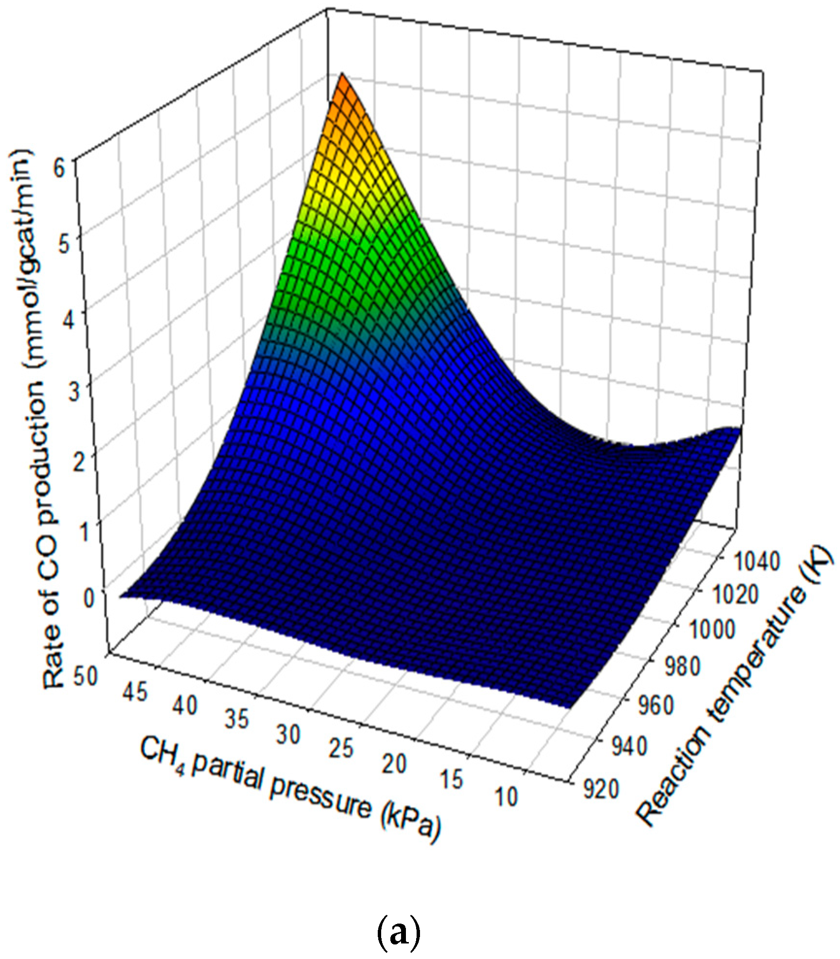
2.3. Interaction Effect of Process Parameters on the Rate CO Production

The interaction effects of CH₄ partial pressure, CO₂ partial pressure, and reaction temperature on the rate of CO production are depicted in Figure 2. At a constant CH₄ partial pressure (Figure 2a), the rate of CO production was steady with increases in the CH₄ partial pressure, whereas a significant increase in the rate of CO production was observed with an increase in the reaction temperature, which agrees with the Arrhenius theory for temperature-dependent gas phase reactions. Based on Figure 2a, the CH₄ partial pressure did not have much influence on the rate of CO production. This is due to the fact that CO is solely produced from the activation of CO₂. At a lower CH₄ partial pressure, it can be inferred that the Bondouard reaction is dominant [36]. In this case, the CO produced was subsequently converted to CO₂ and carbon. However, as the CH₄ partial pressure increased, a state of equilibrium was attained with the CO₂ partial pressure, thereby resulting in an increase in the rate of CO production. A similar trend can be observed in Figure 2b, although there was a steady increase in the rate of CO production at a lower PCO₂ partial pressure, as reported by Foo et al. [33]. The interaction between CO₂ and the CH₄ partial pressure had a significant influence on the rate of CO production. However, the CO₂ partial pressure has the most significant influence on the rate of CO production, which is consistent with the fact that CO is produced during the activation of CO₂.

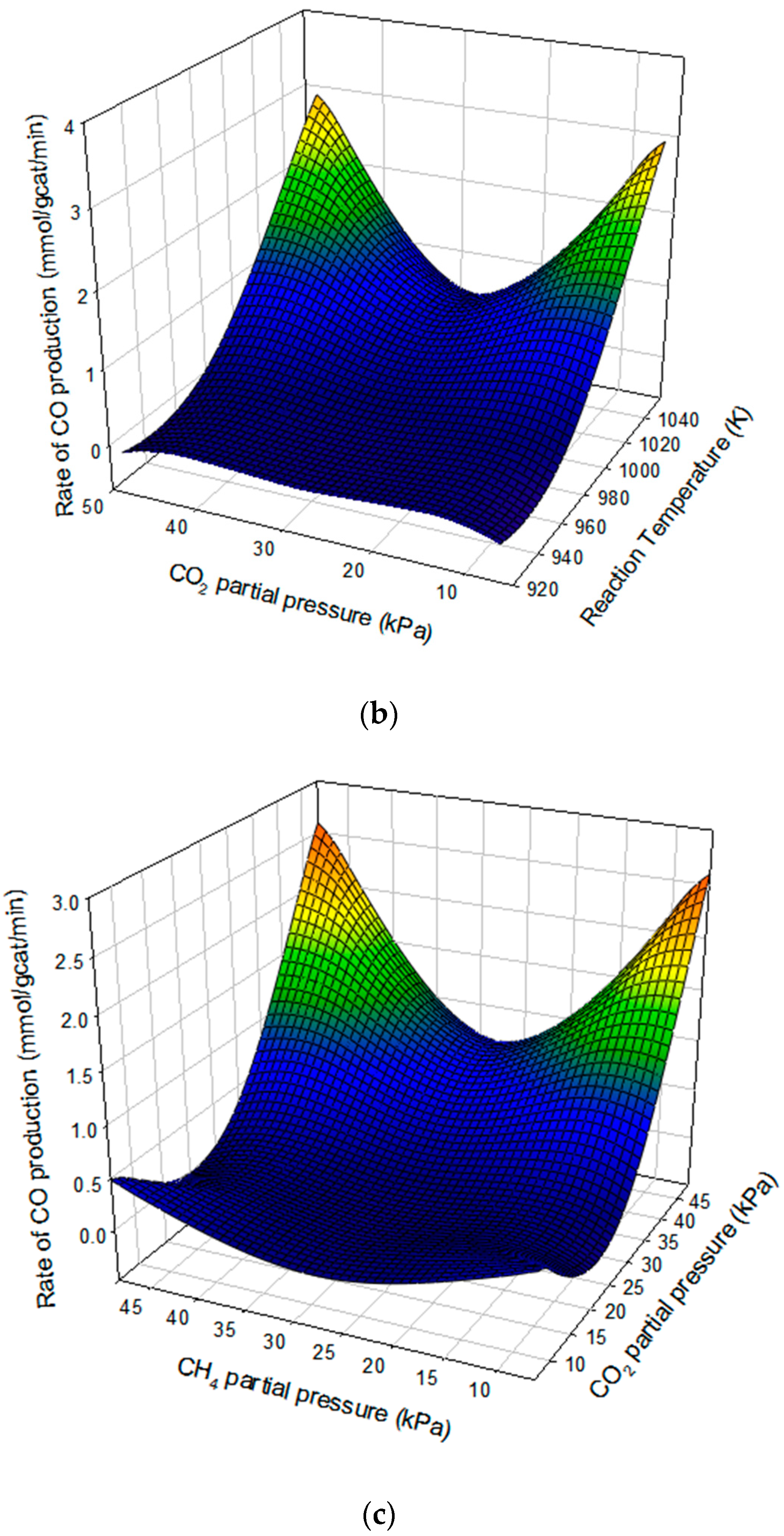
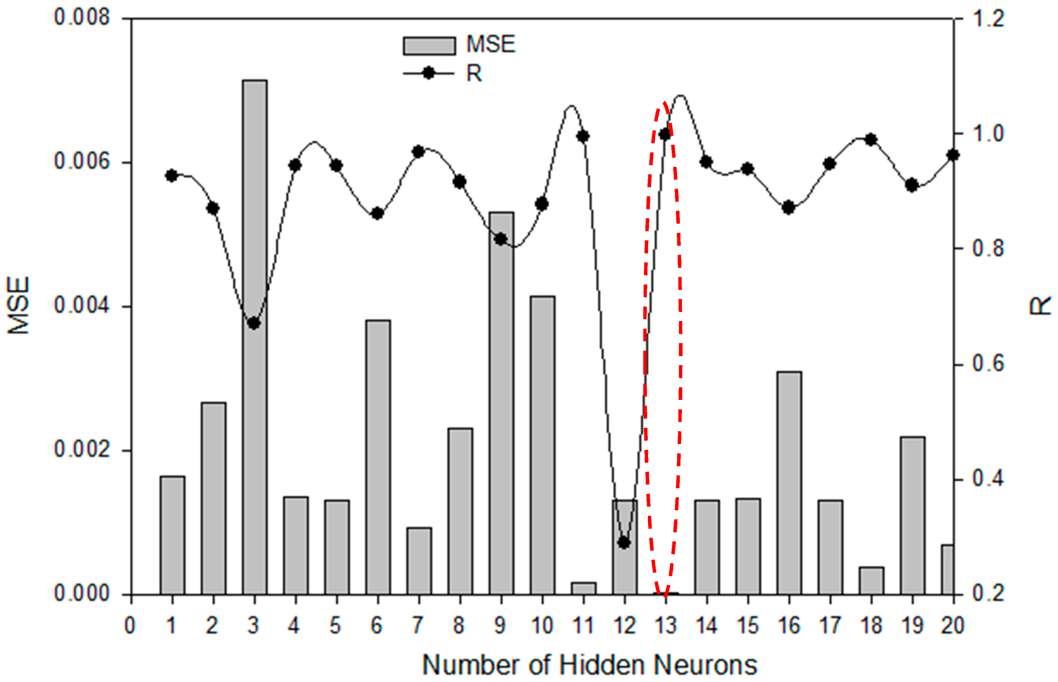
2.4. Artificial Neural Network Modeling

Prior to the commencement of the network analysis, several ANN configurations were trained in other to determine the most suitable hidden neuron that minimized the MSE. As shown in Figure 3, Figure 4 and Figure 5, the best ANN architecture for each of the training algorithms was obtained at the least MSE. The values of the MSE varied with changes in the number of hidden neurons. Hidden neuron ranges from 1 to 20 were tested for each of the algorithms, which resulted in the best hidden neuron of 13, 15, and 15 for Leven–Marquardt, Bayesian regularization, and scaled conjugate gradient algorithms, respectively. MSE values of 1.91 × 10⁻⁵, 5.65 × 10⁻⁴, and 9.34 × 10⁻⁴ were obtained for the ANN architecture using Leven–Marquardt, Bayesian regularization, and scaled conjugate gradient algorithms, respectively. The high R values of 0.998, 0.977, and 0.956 revealed that the predicted rate of CO and H₂ at the obtained lowest MSE were very close to the actual values (

Table 2. Determination of the best neuron for each of the training algorithms.

Hidden Neuron	Leven–Marquardt		Bayesian Regularization		Scaled Conjugate Gradient
	MSE	R	MSE	R	MSE	R
1	1.63 × 10−3	0.927	2.47 × 10−3	0.860	7.47 × 10−3	0.647
2	2.67 × 10−3	0.870	1.21 × 10−3	0.949	3.75 × 10−3	0.840
3	7.14 × 10−3	0.671	1.19 × 10−3	0.950	6.93 × 10−3	0.690
4	1.36 × 10−3	0.945	1.21 × 10−3	0.958	7.98 × 10−3	0.853
5	1.32 × 10−3	0.943	6.12 × 10−4	0.973	2.94 × 10−3	0.877
6	3.81 × 10−3	0.861	5.67 × 10−4	0.976	2.18 × 10−3	0.909
7	9.39 × 10−4	0.967	1.10 × 10−3	0.954	2.92 × 10−3	0.879
8	2.31 × 10−3	0.916	1.12 × 10−3	0.949	2.93 × 10−3	0.887
9	5.31 × 10−3	0.816	1.13 × 10−3	0.955	1.97 × 10−3	0.919
10	4.14 × 10−3	0.877	5.66 × 10−4	0.976	1.91 × 10−3	0.929
11	1.57 × 10−4	0.994	1.13 × 10−3	0.953	1.81 × 10−3	0.915
12	1.32 × 10−3	0.290	1.11 × 10−3	0.953	9.51 × 10−3	0.651
13	1.91 × 10−5	0.998	1.12 × 10−3	0.951	1.39 × 10−3	0.946
14	1.31 × 10−3	0.949	1.11 × 10−3	0.954	2.39 × 10−3	0.895
15	1.33 × 10−3	0.939	5.65 × 10−4	0.977	9.34 × 10−4	0.956
16	3.09 × 10−3	0.871	5.68 × 10−4	0.976	1.83 × 10−3	0.924
17	1.31 × 10−3	0.947	1.22 × 10−3	0.945	2.01 × 10−3	0.921
18	3.82 × 10−4	0.989	5.84 × 10−4	0.977	4.81 × 10−3	0.823
19	2.19 × 10−3	0.910	1.11 × 10−3	0.951	2.81 × 10−3	0.878
20	6.86 × 10−4	0.963	1.11 × 10−3	0.953	1.83 × 10−3	0.914

).

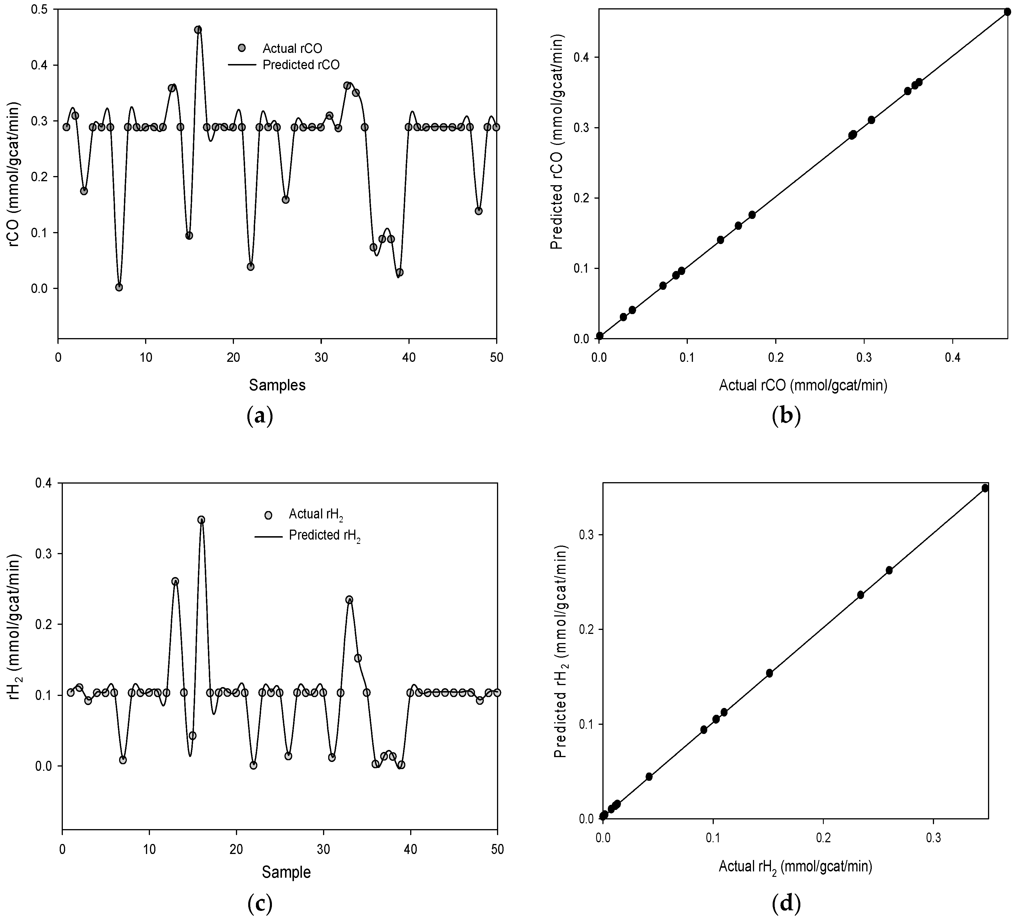
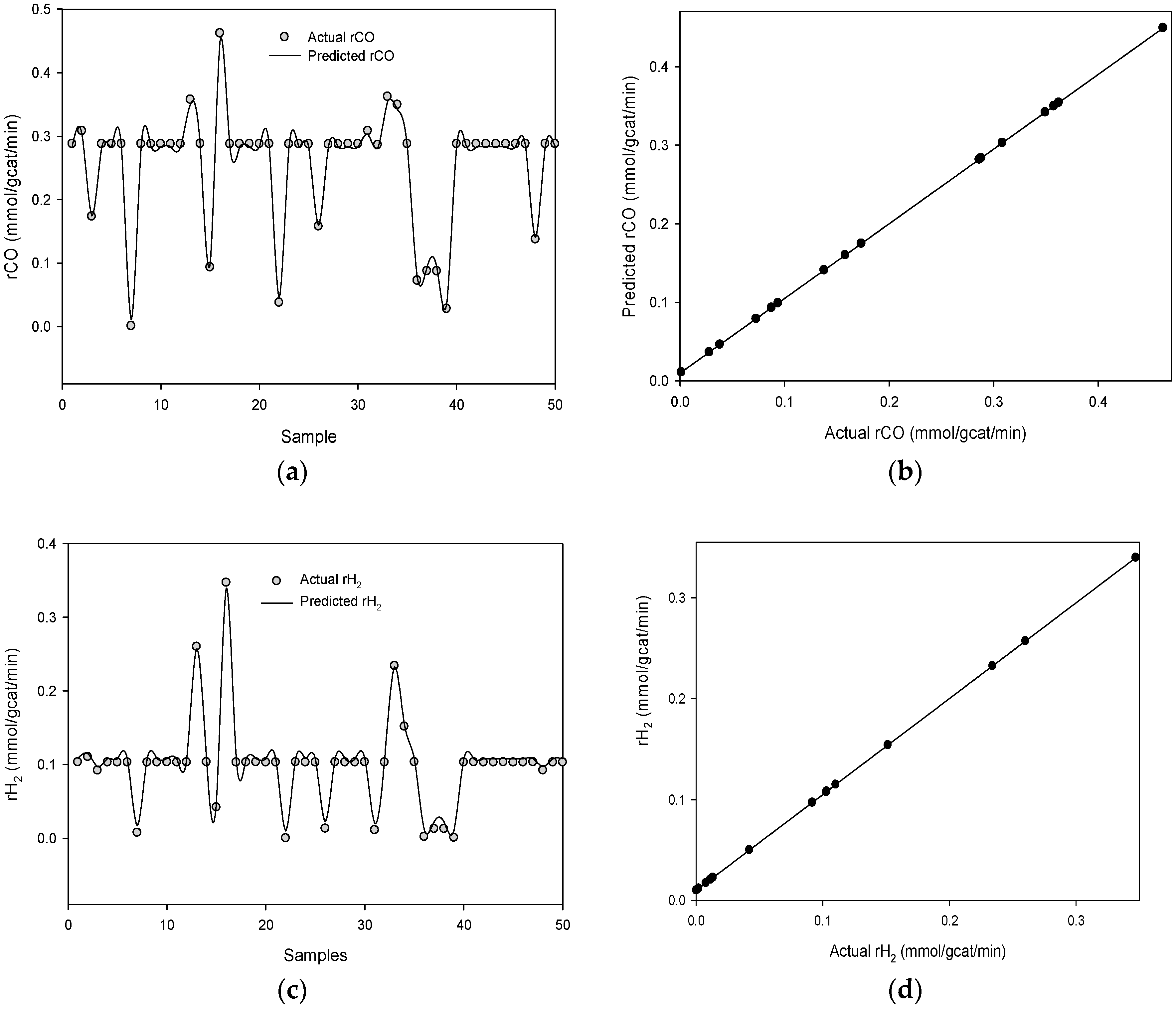
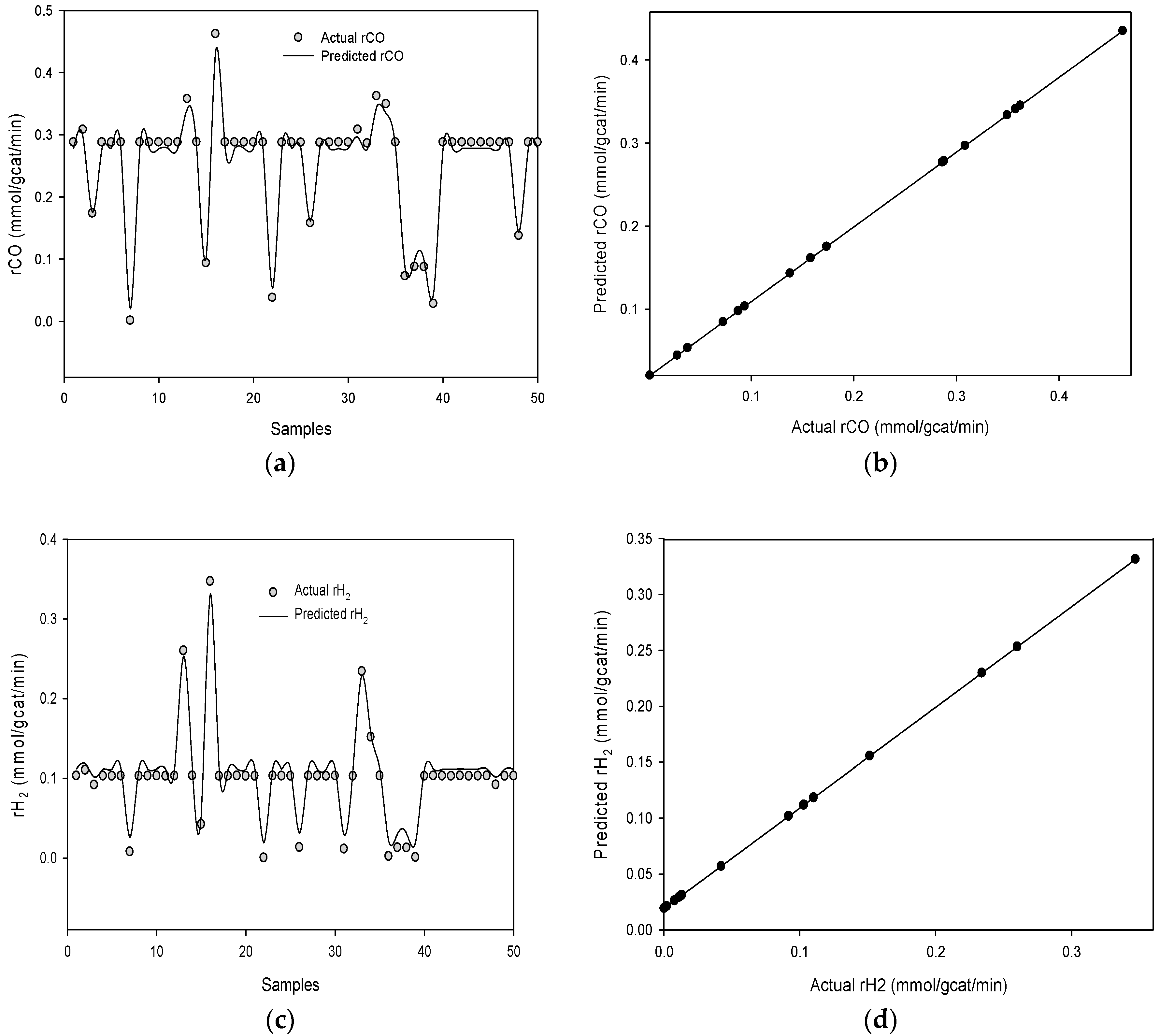
2.5. The ANN Model Predictive Analysis

The performance of the ANN prediction of the rate of H₂ and CO production using the Leven–Marquardt, Bayesian Regularization, and scaled conjugate gradient algorithms are depicted in Figure 6, Figure 7 and Figure 8. Figure 6 depicts the dispersion diagrams and the parity plots showing the actual and the ANN-predicted rates of CO and H₂ production using the Leven–Marquardt algorithm. The filled circles in the dispersion diagrams represent the actual rates of CO and H₂ production, while the spline curves depict the ANN-predicted rates of CO and H₂ production. It can be seen that the use of the Leven–Marquardt algorithm resulted in a good prediction of the rate of CO and H₂ production, as shown in the dispersion diagram (Figure 6a,c). The accuracy of the ANN prediction is further revealed from the parity plot. The actual values of the rate of CO and H₂ production are strongly correlated to the predicted values. Several authors have reported that the Leven–Marquardt algorithm is one of the most effective algorithms used for training ANN models. Its performance is hinged on the advantage of combining both the Gauss–Newton method and the steepest descent technique to attain convergence [37]. Furthermore, the use of the Leven–Marquardt algorithm enables the trained network to rapidly converge near the vicinity of the minimum error [38]. The good prediction of the ANN outputs in this study using the Leven–Marquardt algorithm is consistent with that reported in previous studies. Puig-Arnavat and Bruno [21] employed the Leven–Marquardt algorithm for the modeling of the thermochemical conversion of biomass. The application of the Leven–Marquardt algorithm for training the network resulted in an accurate prediction of H₂ in producer gas, CH₄ in producer gas, CO₂ in producer gas, and CO in producer gas. The predicted values were found to be in good agreement with the actual values based on the parity plots. In a similar study, George et al. [23] applied the Leven–Marquardt algorithm for the predictive modeling of producer gas composition during biomass gasification. The study revealed that the predicted values of the producer gas were in good agreement with the actual values with an R value of 0.987.

The ANN performance using the Bayesian regularization algorithm is represented in the dispersion and parity plots in Figure 7. The use of the Bayesian regularization algorithm for ANN training is founded on the probabilistic understanding of the network parameters [38]. It employs an optimum set of weights for the minimization of the error function [39]. As shown in Figure 7 the use of the Bayesian regularization also displayed a good prediction of the rate of CO and H₂ production. The dispersion diagrams in Figure 7a,c reveal the proximity between the predicted rate CO and H₂ production, while the parity plots (Figure 7b,d) show that both the predicted CO and H₂ production are in good agreement. Studies have shown that the use of the Bayesian regulation algorithm for ANN modeling results in a good prediction of the targets. George et al. [23] employed the Bayesian regularization algorithm for the ANN modeling of wheat output energy from a wheat production process. The study revealed that the use of the Bayesian regularization algorithm resulted in a good prediction of the wheat output energy which was in good agreement with the actual values. Shi et al. [40] applied the Bayesian regularization algorithm in the ANN modeling of explosion risk analysis of a fixed offshore platform. The Bayesian regulation-trained ANN accurately predicted the cumulative frequency of the maximum overpressure.

The performance of the scaled conjugate gradient algorithm-trained ANN is represented in the dispersion diagrams and parity plots in Figure 8. The scaled conjugate gradient algorithm employed step size scaling mechanism which make it have a very fast iteration [41]. As depicted in Figure 8a,c, the use of the scaled conjugate gradient algorithm for ANN modeling resulted in a good prediction of the rate of CO and H₂ production. The predicted values of the rate of CO and H₂ production are in good agreement with the actual values as depicted by the parity plots in Figure 8b,d. The good prediction of the rate of CO and H₂ production obtained in this study is consistent with that reported by Khadse et al. [41] who employed the scaled conjugate gradient algorithm for the ANN modeling of an electromagnetic compatibility estimator. The authors revealed that the use of the scaled conjugate gradient algorithm for ANN modeling produced an accurate prediction of the output. Similarly, Mia and Dhar [39] also confirmed the robustness of the scaled conjugate gradient as a training algorithm for ANN predictive modeling of surface roughness in hard turning under high-pressure coolant. The prediction of the surface roughness using the scaled conjugate gradient-trained ANN model was in good agreement the actual values.

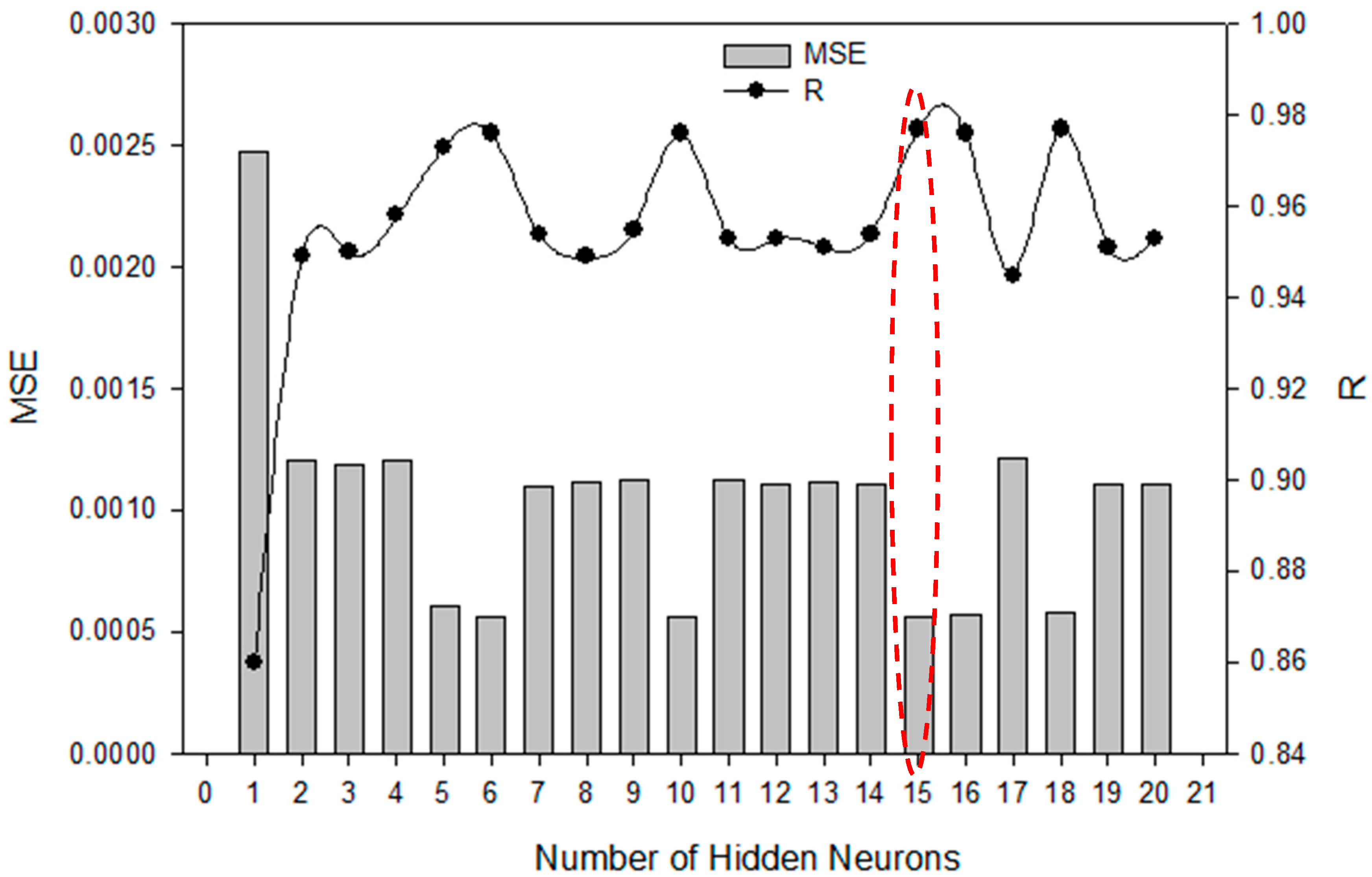
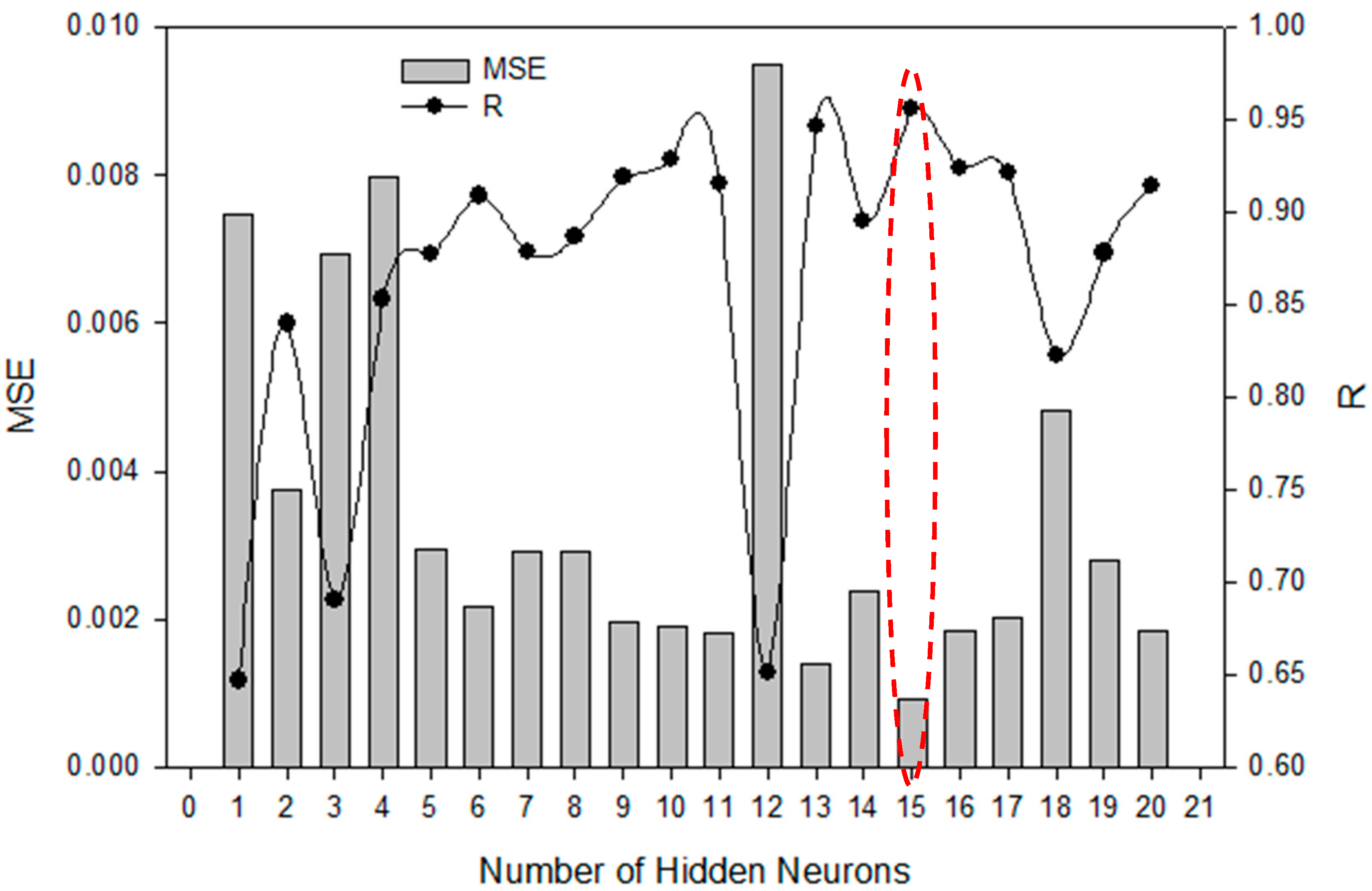
2.6. Comparison of the Leven–Marquardt, Bayesian Regularization, and Scaled Conjugate Gradient Algorithms

The comparison of the ANN model using the Leven–Marquardt, Bayesian regularization, and scaled conjugate gradient algorithms using statistical parameters is depicted in

Table 3. Statistical analysis of the ANN modeling using different algorithms.

	Leven–Marquardt		Bayesian Regularization		Scaled Conjugate Gradient
	rCO	rH2	rCO	rH2	rCO	rH2
SEE	2.54 × 10−17	1.0607 × 10−17	2.0526 × 10	9.9084 × 10−18	2.80 × 10−17	7.77 × 10−18
R2	0.9992	0.9992	0.9726	0.9726	0.9565	0.9565
Model Equation	Output = 1×Target + 0.0018	Output = 1×Target + 0.0018	Output = 0.95×Target + 0.0099	Output = 0.95×Target + 0.0099	Output = 0.9×Target + 0.019	Output = 0.9×Target + 0.019

. Statistical parameters, such as the standard error of estimates (SEE) and coefficient of determination (R²) were employed to discriminate between the performance of the three algorithms. The ANN modeling using the Bayesian regularization algorithm resulted in the lowest SEE of 2.0526 × 10⁻¹⁷ obtained from the predicted and the actual rates of CO production compared to the ANN-trained using the Leven–Marquardt and scaled conjugate gradient algorithms. A high R² > 0.9 was obtained for the three algorithms indicating a strong agreement between the predicted rate of CO and the actual values. Nevertheless, the ANN trained with the Leven–Marquardt algorithm displayed the highest R² of 0.9992, which implies that the predicted rate of CO production is in closest agreement compared to the other two algorithms. On the contrary, the ANN trained with the scaled conjugate gradient algorithm produced the lowest SEE of 7.77 × 10⁻¹⁸ from the prediction of rate of H₂ production compared to Leven–Marquardt and scaled conjugate gradient algorithms. Although, all three algorithms used for the ANN training resulted in high R² > 0.9, the R² of 0.992 obtained using the Leven–Marquardt algorithm shows that the predicted and actual values of the rate of H₂ production are in closer agreement compared to the other two algorithms which have lower R² values. Mia and Dhar [39] compared the use of the Leven–Marquardt, Bayesian regularization, and scaled conjugate gradient algorithms for the predictive modeling of surface roughness in hard turning under high-pressure coolant using ANN. The results show that the Bayesian regularization-trained ANN presented the lowest root mean square errors with R² of 0.997.

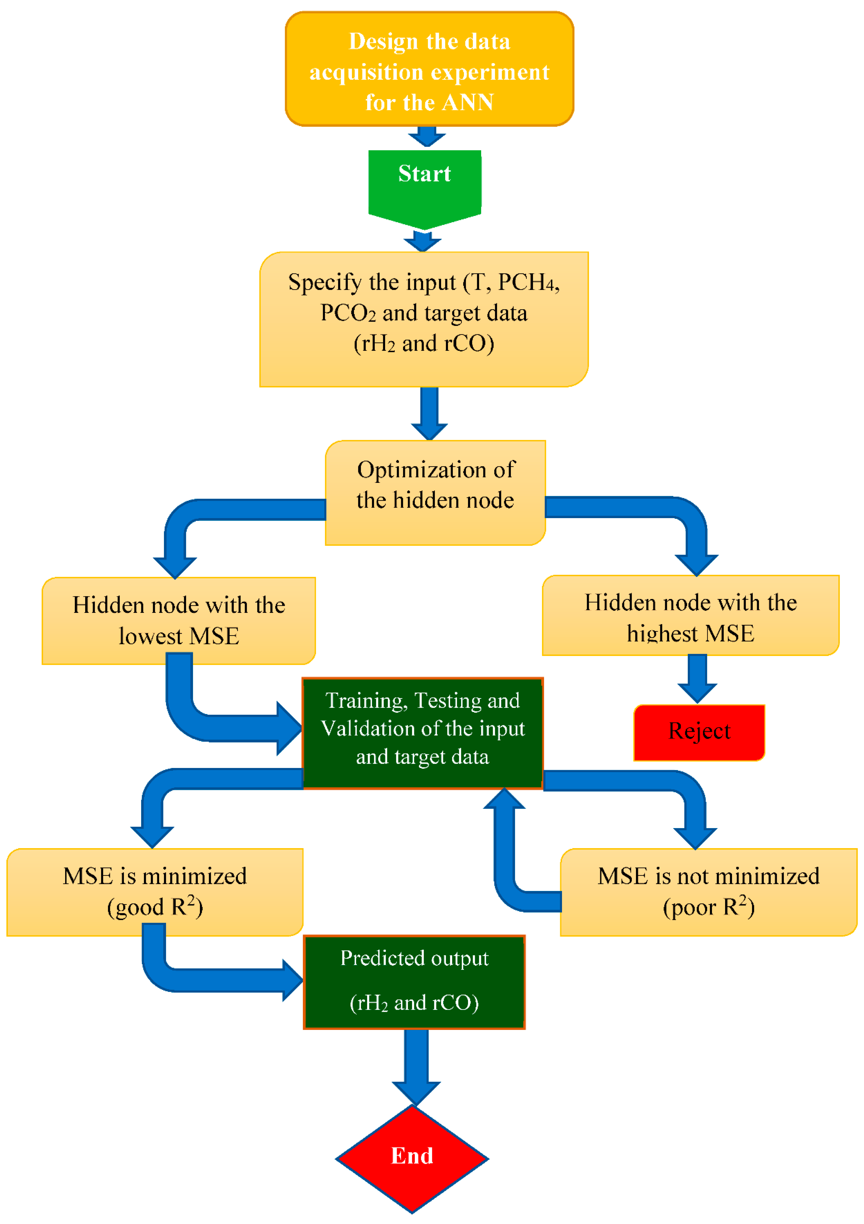
3. Data Acquisition for ANN Modeling

Figure 9 shows the schematic representation of the stages involved in the data acquisition and the ANN modeling of the rate of H₂ and CO production. Basically, there are five stages involved, from the data acquisition for the ANN to the prediction of the output. The data used for the ANN modeling was obtained from experimental runs designed by employing a central composite design (CCD). The input variables for the experimental design include CH₄ partial pressure, CO₂ partial pressure, and reaction temperature while the rate of hydrogen (rH₂) and rate of CO (rCO) production were the output variables. Each of the output variables were obtained from the treatment combinations of the three input parameters.

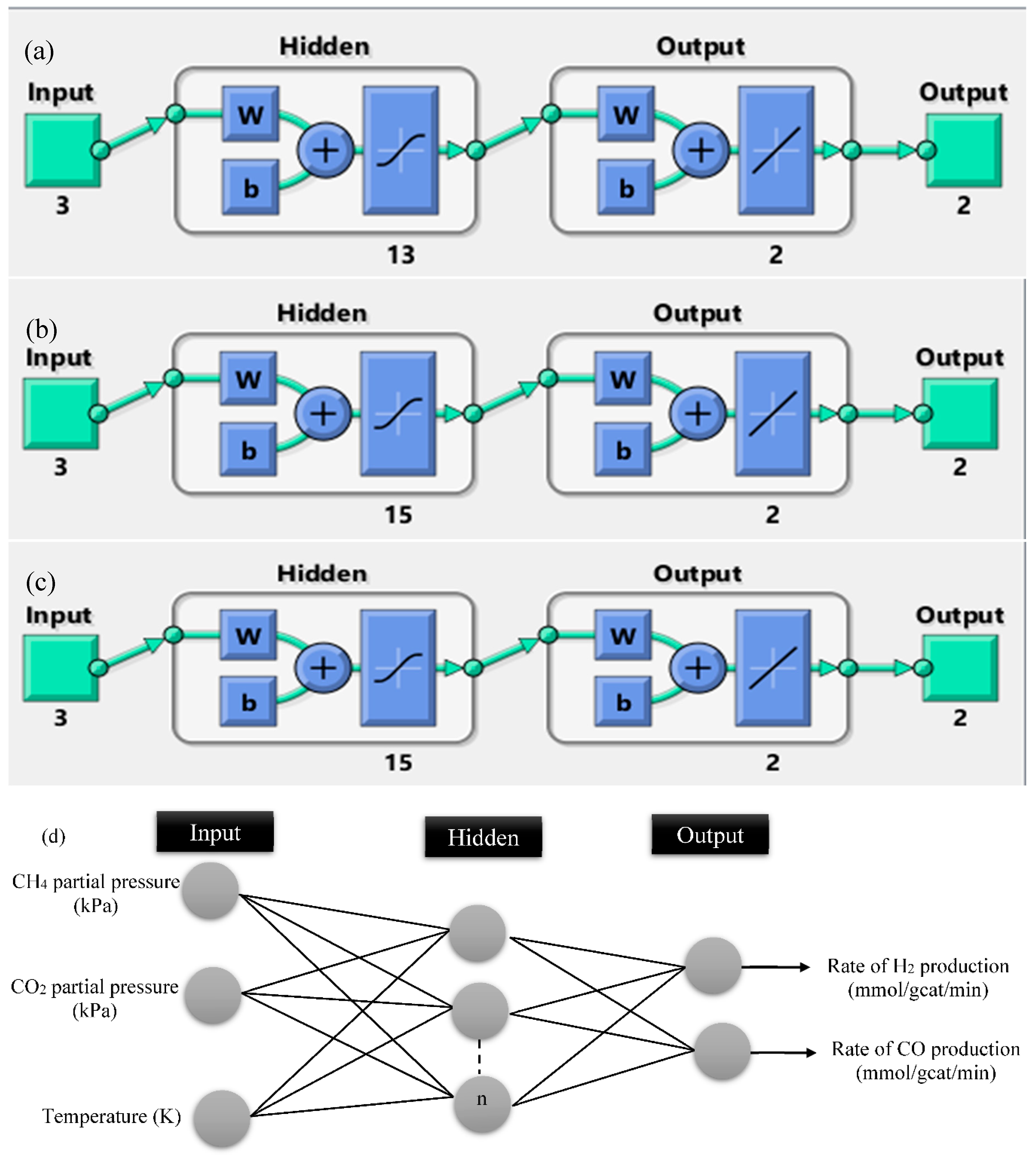
3.1. Artificial Neural Network Configurations

The ANN is an artificial intelligent model that is developed to mimic the pattern of processing information by the human brain [42]. The neural network configuration processes a large number of interlinked units arranged in layers. The interlinked units are patterned after the human neuron and they consist of the input layer, the hidden layers, and the output layers (also known as the target) [18]. Each of the interlinked units have varying connection strengths, known as weights. The ANN functions in such a way that each of the input signals is multiplied with the corresponding connection weights to obtain a combined weighted hidden layer [43]. The combined hidden layers are subsequently passed through an activation function which in turn generates the corresponding output. The Sigmoid function represented in Equation (2) is the most commonly use form of an activation function [20].

$$f\left(Z_i\right)= \frac{1}{1+e^{-Z_i}}$$

(2)

where $Z_i$ represents the summation of each of the hidden layers multiplied by an assigned weight plus bias from each neuron in the previous layer. Just like the human brain, the neural network model functions by exploring the non-linear relationship between the individual input and the target data. Subsequently, the network model creates a predicted output with minimized error. For an incorrect prediction, the weights are adjusted in a circle of iteration to produce an output with minimum error.

The manner of connection of the hidden neuron in an ANN is crucial to the performance of the network model. The neuron can either be connected in such a way to give a feedforward signals or a feedback signal. In this study, a feedforward ANN configuration is adopted due to its wide applicability in the process industries [44,45]. The feedforward ANN is a multilayer perceptron with 2 13 2 2, 2 15 2 2, and 2 15 2 2 architectures for the Leven–Marquardt, Bayesian regularization, and scaled conjugate gradient algorithms, respectively, as shown in Figure 10a–c. The input parameters to the neural network include CH₄ partial pressure, CO₂ partial pressure, and reaction temperature, while the target parameters are rate of H₂ and CO production (Figure 10d). The parameters employed for the ANN configuration are depicted in

Table 4. Configuration parameters for the neural network architecture.

Configuration Parameters	Leven–Marquardt	Bayesian Regularization	Scaled Conjugate Gradient
Algorithm	Feed forward with 3 layers	Feed forward with 3 layers	Feed forward with 3 layers
Hidden layer size	1	1	1
Hidden neuron quantity	13	15	15
Output layer size	2	2	2
Output neuron quantity	2	2	2
Output layer neurons activation	Pure linear	Pure linear	Pure linear
Training ratio	0.01	0.01	0.01
Epochs	5	1000	21
Training target error	0.001	0.001	0.001

.

3.2. Network Training, Testing, and Validation

After applying the necessary configurations to the neural network and the data have been imputed, it is expedient to apply the necessary algorithm for the network training. During network training, the input data presented to the network are compared to the output unit, thereby adjusting the weight of all units based on their errors for an improved prediction. In this study, the network was trained using the Leven–Marquardt, Bayesian regularization, and scaled conjugate gradient algorithms [38,46,47]. The Leven–Marquardt training algorithm utilizes a damping factor which is self-adjusted during each iteration in order to obtain the least error between the predicted and the actual values [38]. The Leven–Marquardt training algorithm has the advantage of attaining a very fast convergence. The Bayesian regularization training algorithm has the tendency to minimize the estimated errors through an inbuilt objective function that contains a residual sum of squares and the sum of squared weighs [40]. Hence, it is typical to obtain a good generalization model using the Bayesian regularization training algorithm [38]. To minimize the errors, the weights in scaled conjugate gradient algorithms are adjusted in the direction in which the network function performance is decreasing most rapidly. More iterations are required for convergence using scaled conjugate gradient algorithms compared to Leven–Marquardt and Bayesian regularization. Testing of the network provides an independent measure of its performance during and after the training. While validation is a form of measuring the network generalization and halting of training when generalization has stopped improving. The training, testing, and validation of the network were performed using the neural network toolbox in MATLAB 2019a (MathWorks Inc., Natick, MA, USA). The data were proportioned into 70%, 15%, and 15% for training, testing, and validation of the network, respectively. The detailed network architectures of the feedforward multilayer perceptron are depicted in Figure 3.

3.3. Evaluation of the ANN Performance

The accuracy of the ANN to predict the rate of CO and H₂ production were measured using parameters such as the mean square error (MSE) and the correlation coefficient (R) [27]. The MSE defined in Equation (3) was used to measure the average squared difference between the predicted rate of CO and H₂ production and the actual values. The lower the MSE values, the more accurate the ANN prediction.

$$MSE= \frac{1}{n}{\sum }_{i=1}^n{〖(Y_p-Y_a〗)}^2$$

(3)

where n is the number of samples, $Y_p$ and $Y_a$ are the predicted and the actual values, respectively.

The correlation coefficient (R) defined in Equation (4) was employed to determine the strength of the linear relationship between the predicted rate of CO and H₂ production and the actual values.

$$R= \frac{1}{n-1}\left[\frac{{\sum }_x {\sum }_y\left(x-\overline{x}\right)\left(y-\overline{y}\right)}{S_x{S}_y}\right]$$

(4)

where n is the number of samples, $\overline{x}$ and $\overline{y}$ are the sample means of all the $x$ and $y$ values. $S_x$ and $S_y$ are the standard deviation of all the $x$ and $y$ values. An R value of 1 implies that a close relationship between the predicted rate of CO and H₂ production and the actual values exists, while an R value of 0 implies that a random relationship exists between the predicted rate of CO and H₂ production and the actual values.

4. Conclusions

In this study, the use of artificial neural network as a predictive model has been investigated. Three algorithms, namely Leven–Marquardt, Bayesian regularization, and scaled conjugate gradient, were employed to train the ANN for the prediction of the rate of CO and H₂ production from methane dry reforming catalyzed by Co/Pr₂O₃. The ANN predictive modeling was performed using datasets obtained from central composite experimental design. Several architectures of the ANN were tested using hidden neurons in the range of 1–20. The best ANN architectures were obtained using 13, 15, and 15 hidden neurons for Leven–Marquardt, Bayesian regularization, and scaled conjugate gradient algorithms, respectively. The training of the ANN model with the best neurons results in good predictions of the rates of CO and H₂ production using the three training algorithms. The R² values of 0.9992, 0.9726, and 0.9565 obtained using the Leven–Marquardt, Bayesian regularization, and scaled conjugate gradient algorithms, respectively, are an indication that the predicted rates of CO and H₂ production were in good agreement with the observed values. However, the best prediction was obtained using the Bayesian regularization training algorithm for the ANN model. This study has demonstrated the use of ANN predictive modeling to investigate the functional relationship that exists between the process parameters in the production of CO-rich hydrogen by a methane dry reforming reaction over a Co/Pr₂O₃ catalyst.

References

1. Ayodele, B.V.; Khan, M.R.; Lam, S.S.; Cheng, C.K. Production of CO-rich hydrogen from methane dry reforming over lanthania-supported cobalt catalyst: Kinetic and mechanistic studies. Int. J. Hydrogen Energy 2016, 41, 4603–4615. [Google Scholar] [CrossRef] [Green Version]
2. Ashraf, M.A.; Sanz, O.; Montes, M.; Specchia, S. Insights into the effect of catalyst loading on methane steam reforming and controlling regime for metallic catalytic monoliths. Int. J. Hydrogen Energy 2018, 43, 11778–11792. [Google Scholar] [CrossRef]
3. Heng, L.; Xiao, R.; Zhang, H. Life cycle assessment of hydrogen production via iron-based chemical-looping process using non-aqueous phase bio-oil as fuel. Int. J. Greenh. Gas Control 2018, 76, 78–84. [Google Scholar] [CrossRef]
4. Bulutoglu, P.S.; Say, Z.; Bac, S.; Ozensoy, E.; Avci, A.K. Dry reforming of glycerol over Rh-based ceria and zirconia catalysts: New insights on catalyst activity and stability. Appl. Catal. A Gen. 2018, 564, 157–171. [Google Scholar] [CrossRef]
5. Sengodan, S.; Lan, R.; Humphreys, J.; Du, D.; Xu, W.; Wang, H.; Tao, S. Advances in reforming and partial oxidation of hydrocarbons for hydrogen production and fuel cell applications. Renew. Sustain. Energy Rev. 2018, 82, 761–780. [Google Scholar] [CrossRef]
6. Ayodele, B.V.; Khan, M.R.; Cheng, C.K. Greenhouse gases mitigation by CO2 reforming of methane to hydrogen-rich syngas using praseodymium oxide supported cobalt catalyst. Clean Technol. Environ. Policy 2016, 19, 795–807. [Google Scholar] [CrossRef] [Green Version]
7. Ayodele, B.V.; Khan, M.R.; Nooruddin, S.S.; Cheng, C.K. Modelling and optimization of syngas production by methane dry reforming over samarium oxide supported cobalt catalyst: Response surface methodology and artificial neural networks approach. Clean Technol. Environ. Policy 2016, 19, 1181–1193. [Google Scholar] [CrossRef]
8. Abatzoglou, N.; Fauteux-lefebvre, C. Review of catalytic syngas production through steam or dry reforming and partial oxidation of studied liquid compunds. WIREs Energy Environ. 2016, 5, 169–187. [Google Scholar] [CrossRef]
9. Shah, Y.T.; Gardner, T.H. Dry Reforming of Hydrocarbon Feedstocks. Catal. Rev. 2014, 56, 476–536. [Google Scholar] [CrossRef]
10. Abdullah, B.; Abd Ghani, N.A.; Vo, D.V.N. Recent advances in dry reforming of methane over Ni-based catalysts. J. Clean. Prod. 2017, 162, 170–185. [Google Scholar] [CrossRef] [Green Version]
11. Sehested, J. Four challenges for nickel steam-reforming catalysts. Catal. Today 2006, 111, 103–110. [Google Scholar] [CrossRef]
12. San-José-Alonso, D.; Juan-Juan, J.; Illán-Gómez, M.J.; Román-Martínez, M.C. Ni, Co and bimetallic Ni-Co catalysts for the dry reforming of methane. Appl. Catal. A Gen. 2009, 371, 54–59. [Google Scholar] [CrossRef]
13. Huang, X.; Ji, C.; Wang, C.; Xiao, F.; Zhao, N.; Sun, N.; Wei, W.; Sun, Y. Ordered mesoporous CoO-NiO-Al2O3 bimetallic catalysts with dual confinement effects for CO2 reforming of CH4. Catal. Today 2016, 281, 241–249. [Google Scholar] [CrossRef]
14. Ayodele, B.V.; Khan, M.R.; Cheng, C.K. Production of CO-rich hydrogen gas from methane dry reforming over Co/CeO2 Catalyst. Bull. Chem. React. Eng. Catal. 2016, 11, 210–219. [Google Scholar] [CrossRef]
15. Ayodele, B.V.; Khan, M.R.; Cheng, C.K. Syngas production from CO2 reforming of methane over ceria supported cobalt catalyst: Effects of reactants partial pressure. J. Nat. Gas Sci. Eng. 2015, 27, 1016–1023. [Google Scholar] [CrossRef]
16. Ayodele, B.V.; Khan, M.R.; Cheng, C.K. Catalytic performance of ceria-supported cobalt catalyst for CO-rich hydrogen production from dry reforming of methane. Int. J. Hydrogen Energy 2015, 41, 198–207. [Google Scholar] [CrossRef]
17. Kathiraser, Y.; Oemar, U.; Saw, E.T.; Li, Z.; Kawi, S. Kinetic and mechanistic aspects for CO 2 reforming of methane over Ni based catalysts. Chem. Eng. J. 2015, 278, 62–78. [Google Scholar] [CrossRef]
18. Hossain, M.A.; Ayodele, B.V.; Cheng, C.K.; Khan, M.R. Artificial neural network modeling of hydrogen-rich syngas production from methane dry reforming over novel Ni/CaFe2O4 catalysts. Int. J. Hydrogen Energy 2016, 41, 11119–11130. [Google Scholar] [CrossRef] [Green Version]
19. Ayodele, B.V.; Cheng, C.K. Modelling and optimization of syngas production from methane dry reforming over ceria-supported cobalt catalyst using artificial neural networks and Box-Behnken design. J. Ind. Eng. Chem. 2015, 32, 246–258. [Google Scholar] [CrossRef]
20. Arce-Medina, E.; Paz-Paredes, J.I. Artificial neural network modeling techniques applied to the hydrodesulfurization process. Math. Comput. Model. 2009, 49, 207–214. [Google Scholar] [CrossRef]
21. Puig-Arnavat, M.; Bruno, J.C. Artificial Neural Networks for Thermochemical Conversion of Biomass. Recent Adv. Thermochem. Conver. Biomass 2015, 133–156. [Google Scholar] [CrossRef] [Green Version]
22. Ghasemzadeh, K.; Ahmadnejad, F.; Aghaeinejad-Meybodi, A.; Basile, A. Hydrogen production by a Pd—Ag membrane reactor during glycerol steam reforming: ANN modeling study. Int. J. Hydrogen Energy 2018, 43, 7722–7730. [Google Scholar] [CrossRef]
23. George, J.; Arun, P.; Muraleedharan, C. Assessment of producer gas composition in air gasification of biomass using artificial neural network model. Int. J. Hydrogen Energy 2018, 43, 9558–9568. [Google Scholar] [CrossRef]
24. Basile, A.; Curcio, S.; Bagnato, G.; Liguori, S.; Jokar, S.M.; Iulianelli, A. Water gas shift reaction in membrane reactors: Theoretical investigation by artificial neural networks model and experimental validation. Int. J. Hydrogen Energy 2015, 40, 5897–5906. [Google Scholar] [CrossRef]
25. Shahbaz, M.; Taqvi, S.A.; Minh Loy, A.C.; Inayat, A.; Uddin, F.; Bokhari, A.; Naqvi, S.R. Artificial neural network approach for the steam gasification of palm oil waste using bottom ash and CaO. Renew. Energy 2019, 132, 243–254. [Google Scholar] [CrossRef]
26. Nasr, N.; Hafez, H.; El, M.H.; Nakhla, G. Application of artificial neural networks for modeling of biohydrogen production. Int. J. Hydrogen Energy 2013, 38, 3189–3195. [Google Scholar] [CrossRef] [Green Version]
27. Zamaniyan, A.; Joda, F.; Behroozsarand, A.; Ebrahimi, H. Application of artificial neural networks (ANN) for modeling of industrial hydrogen plant. Int. J. Hydrogen Energy 2013, 38, 6289–6297. [Google Scholar] [CrossRef]
28. Ghasemzadeh, K.; Aghaeinejad-Meybodi, A.; Basile, A. Hydrogen production as a green fuel in silica membrane reactor: Experimental analysis and artificial neural network modeling. Fuel 2018, 222, 114–124. [Google Scholar] [CrossRef]
29. Usman, M.; Daud, W.M.A.W.; Abbas, H.F. Dry reforming of methane: Influence of process parameters—A review. Renew. Sustain. Energy Rev. 2015, 45, 710–744. [Google Scholar] [CrossRef]
30. Sun, Y.; Ritchie, T.; Hla, S.S.; McEvoy, S. Thermodynamic analysis of mixed and dry reforming of methane for solar thermal applications. J. Nat. Gas Chem. 2011, 20, 568–576. [Google Scholar] [CrossRef]
31. Ayodele, B.V.; Cheng, C.K. Process modelling, thermodynamic analysis and optimization of dry reforming, partial oxidation and auto-thermal methane reforming for hydrogen and syngas production. Chem. Prod. Process Model. 2015, 10, 211–220. [Google Scholar] [CrossRef]
32. Pakhare, D.; Schwartz, V.; Abdelsayed, V.; Haynes, D.; Shekhawat, D.; Poston, J.; Spivey, J. Kinetic and mechanistic study of dry (CO2) reforming of methane over Rh-substituted La2Zr2O7 pyrochlores. J. Catal. 2014, 316, 78–92. [Google Scholar] [CrossRef]
33. Foo, S.Y.; Cheng, C.K.; Nguyen, T.-H.; Adesina, A.A. Kinetic study of methane CO2 reforming on Co–Ni/Al2O3 and Ce–Co–Ni/Al2O3 catalysts. Catal. Today 2011, 164, 221–226. [Google Scholar] [CrossRef]
34. Aquilanti, V.; Mundim, K.C.; Elango, M.; Kleijn, S.; Kasai, T. Temperature dependence of chemical and biophysical rate processes: Phenomenological approach to deviations from Arrhenius law. Chem. Phys. Lett. 2010, 498, 209–213. [Google Scholar] [CrossRef]
35. Maneerung, T.; Hidajat, K.; Kawi, S. Co-production of hydrogen and carbon nanofibers from catalytic decomposition of methane over LaNi(1-x)Mx O3-α perovskite (where M = Co, Fe and X = 0, 0.2, 0.5, 0.8, 1). Int. J. Hydrogen Energy 2015, 40, 13399–13411. [Google Scholar] [CrossRef]
36. Chen, D.; Lødeng, R.; Anundskås, A.; Olsvik, O.; Holmen, A. Deactivation during carbon dioxide reforming of methane over Ni catalyst: Microkinetic analysis. Chem. Eng. Sci. 2001, 56, 1371–1379. [Google Scholar] [CrossRef]
37. Cui, M.; Yang, K.; Xu, X.L.; Wang, S.D.; Gao, X.W. A modified Levenberg-Marquardt algorithm for simultaneous estimation of multi-parameters of boundary heat flux by solving transient nonlinear inverse heat conduction problems. Int. J. Heat Mass Transf. 2016, 97, 908–916. [Google Scholar] [CrossRef]
38. Kayri, M. Predictive Abilities of Bayesian Regularization and Levenberg–Marquardt Algorithms in Artificial Neural Networks: A Comparative Empirical Study on Social Data. Math. Comput. Appl. 2016, 21, 20. [Google Scholar] [CrossRef]
39. Mia, M.; Dhar, N.R. Prediction of surface roughness in hard turning under high pressure coolant using Artificial Neural Network. Meas. J. Int. Meas. Confed. 2016, 92, 464–474. [Google Scholar] [CrossRef]
40. Shi, J.; Zhu, Y.; Khan, F.; Chen, G. Application of Bayesian Regularization Artificial Neural Network in explosion risk analysis of fixed offshore platform. J. Loss Prev. Process Ind. 2019, 57, 131–141. [Google Scholar] [CrossRef]
41. Khadse, C.B.; Chaudhari, M.A.; Borghate, V.B. Electromagnetic Compatibility Estimator Using Scaled Conjugate Gradient Backpropagation Based Artificial Neural Network. IEEE Trans. Ind. Inform. 2017, 13, 1036–1045. [Google Scholar] [CrossRef]
42. Li, H.; Zhang, Z.; Liu, Z. Application of Artificial Neural Networks for Catalysis: A Review. Catalysts 2017, 7, 306. [Google Scholar] [CrossRef]
43. Bustillo, A.; Pimenov, D.Y.; Matuszewski, M.; Mikolajczyk, T. Using artificial intelligence models for the prediction of surface wear based on surface isotropy levels. Robot. Comput. Integr. Manuf. 2018, 53, 215–227. [Google Scholar] [CrossRef]
44. Benardos, P.G.; Vosniakos, G.C. Optimizing feedforward artificial neural network architecture. Eng. Appl. Artif. Intell. 2007, 20, 365–382. [Google Scholar] [CrossRef]
45. Onalo, D.; Adedigba, S.; Khan, F.; James, L.A.; Butt, S. Data driven model for sonic well log prediction. J. Pet. Sci. Eng. 2018, 170, 1022–1037. [Google Scholar] [CrossRef]
46. Du, Y.C.; Stephanus, A. Levenberg-marquardt neural network algorithm for degree of arteriovenous fistula stenosis classification using a dual optical photoplethysmography sensor. Sensors (Switzerland) 2018, 18, 2322. [Google Scholar] [CrossRef]
47. Sharma, B.; Venugopalan, K. Comparison of Neural Network Training Functions for Hematoma Classification in Brain CT Images. IOSR J. Comput. Eng. 2014, 16, 31–35. [Google Scholar] [CrossRef]
Figure 1. (a) Interaction effect of CH4 partial pressure and reaction partial pressure on the rate of CO production; (b) Interaction effect of CO2 partial pressure and reaction temperature on the rate of CO production; (c) Interaction effect of CH4 partial pressure and CO2 partial pressure on the rate of CO production.
Catalysts 09 00738 g001
Figure 2. (a) Interaction effect of CH4 partial pressure and reaction partial pressure on the rate of H2 production; (b) Interaction effect of CO2 partial pressure and reaction temperature on the rate of H2 production; (c) Interaction effect of CH4 partial pressure and CO2 partial pressure on the rate of H2 production.
Catalysts 09 00738 g002aCatalysts 09 00738 g002b
Figure 3. Determination of the optimized hidden neuron with the minimum mean square error (MSE) for ANN training using the Leven–Marquardt algorithm.
Catalysts 09 00738 g003
Figure 4. Determination of the optimized hidden neuron with the minimum MSE for ANN training using the Bayesian regularization algorithm.
Catalysts 09 00738 g004
Figure 5. Determination of the optimized hidden neuron with the minimum MSE for ANN training using the scaled conjugate gradient algorithm.
Catalysts 09 00738 g005
Figure 6. (a) Dispersion plot showing the comparison between actual and predicted rCO; (b) Parity plots showing the comparison between actual and predicted rCO; (c) Dispersion plot showing the comparison between actual and predicted rH2; (d) Parity plots the comparison between actual and predicted rH2 using Leven–Marquardt algorithm.
Catalysts 09 00738 g006
Figure 7. (a) Dispersion plot showing the comparison between actual and predicted rCO; (b) Parity plots showing the comparison between actual and predicted rCO; (c) Dispersion plot showing the comparison between actual and predicted rH2; (d) Parity plots the comparison between actual and predicted rH2 using Bayesian regularization algorithm.
Catalysts 09 00738 g007
Figure 8. (a) Dispersion plot showing the comparison between actual and predicted rCO; (b) Parity plots showing the comparison between actual and predicted rCO; (c) Dispersion plot showing the comparison between actual and predicted rH2; (d) Parity plots the comparison between actual and predicted rH2 using scaled conjugate gradient algorithm.
Catalysts 09 00738 g008
Figure 9. Flow diagram for the ANN modeling.
Catalysts 09 00738 g009
Figure 10. The Network architecture for the ANN modeling used. (a) Feed forward multi-layer perceptron architecture for prediction of CO-H2 production; (b) Network configuration using the Leven–Marquardt training algorithm; (c) Network configuration using the Bayesian regularization training algorithm; (d) Network configuration using the scaled conjugate gradient training algorithm.
Catalysts 09 00738 g010