The Genetic Algorithm: Using Biology to Compute Liquid Crystal Director Configurations


1
Department of Physics & Astronomy, Swarthmore College, Swarthmore, PA 19081, USA
2
Department of Physics and Astronomy, University of Pennsylvania, Philadelphia, PA 19104, USA
*
Author to whom correspondence should be addressed.
Crystals 2020, 10(11), 1041; https://0-doi-org.brum.beds.ac.uk/10.3390/cryst10111041
Submission received: 28 October 2020
/
Revised: 11 November 2020
/
Accepted: 14 November 2020
/
Published: 16 November 2020
(This article belongs to the Special Issue In Celebration of Noel A. Clark’s 80th Birthday)
Abstract
:The genetic algorithm is an optimization routine for finding the solution to a problem that requires a function to be minimized. It accomplishes this by creating a population of solutions and then producing “offspring” solutions from this population by combining two “parental” solutions in much the way that the DNA of biological parents is combined in the DNA of offspring. Strengths of the algorithm include that it is simple to implement, no trial solution is required, and the results are fairly accurate. Weaknesses include its slow computational speed and its tendency to find a local minimum that does not represent the global minimum of the function. By minimizing the elastic, surface, and electric free energies, the genetic algorithm is used to compute the liquid crystal director configuration for a wide range of situations, including one- and two-dimensional problems with various forms of boundary conditions, with and without an applied electric field. When appropriate, comparisons are made with the exact solutions. Ways to increase the performance of the algorithm as well as how to avoid various pitfalls are discussed.

1. Introduction
Noel Clark’s research into the connection between biology and liquid crystals (LCs) represents some of his most important recent scientific work. Over a period of a little more than a decade, Noel and his co-workers have discovered the liquid crystal properties and suggested the biological significance of short duplexes of DNA [1,2,3,4,5,6,7,8,9,10,11,12,13]. It all started in 2007 with the discovery that (1) short DNA duplexes spontaneously stack in solution, forming longer assemblies that form liquid crystal phases, and (2) mixtures with uneven concentrations of complementary oligomers phase separate into a liquid crystal phase formed by paired strands and an isotropic phase formed by unpaired strands [1]. The implications of this led the authors to state the following [1].
The formation of the LC phase by the complementary duplexes has the autocatalytic effect of establishing conditions that would strongly promote their own growth into longer complementary chains relative to the non–LC-forming oligomers. The fact that the liquid crystal ordering is found to depend sensitively on complementarity introduces selectivity into this process and means that the overall structure of the complementary assemblies generated will actually be templated by the liquid crystal geometry. This appears to have been the case for the linear rodlike structure of base-paired polynucleotides.
This turned out to be the theme for subsequent work coming from the group. Soon they showed that if unpaired strands dangled from the ends of the duplexes and that if opposite dangling ends were made complementary, the assembly process was even more robust [2]. They even found that oligomers with random base sequences were capable of forming liquid crystal phases [4]. Later, they showed that their initial conjecture of an autocatalytic process was correct by introducing a ligating agent [7]. Again the authors point out the implications of this [7].
The coupling between order-templated ligation and selectivity provided by supramolecular ordering enables an autocatalytic cycle favoring the growth of DNA chains, up to biologically relevant lengths, from few-base long oligomers. This finding suggests a novel scenario for the abiotic origin of nucleic acids.
More recent work demonstrated that even ultra-short DNA duplexes form liquid crystal phases [10], and that nucleic acid monobases by themselves can assemble and form liquid crystal phases [12]. The implication is clear [12].
Liquid crystal autocatalysis, … in which a combination of chromonic LC ordering and chemical activity selects and evolves molecular populations, has the potential to support the onset of an RNA world, by providing a feedstock of chains with diverse side groups capable of stacking and sequence-directed self-assembly, from both monomeric components and recycled deteriorated products.
Since Noel and his colleagues have shown how the liquid crystal phase allows DNA to perform extremely significant functions, it is therefore appropriate to include in this special issue an example of how DNA properties can be utilized to answer questions about the behavior of liquid crystal phases. This is done by making use of the genetic algorithm (GA), a computational technique that is well known and useful in many areas of study. The strength of the GA lies in its ease of use. It can be easily implemented to determine the director configuration of a confined liquid crystal, a very important task in the study and application of liquid crystals. In fact, once a simple routine is written for evaluation of the free energy, multiple situations can be examined with almost no additional overhead. While using the GA to calculate director configurations is by no means the most powerful and accurate method, it does produce reasonable solutions for a variety of situations without the need for extensive programming, even when the director configuration is basically unknown.
The basics of elasticity theory of nematic LCs are first discussed, followed by a more detailed description of the genetic algorithm. Then its implementation in MATLAB is described along with useful ideas on obtaining accurate solutions. Six examples are used to demonstrate exactly how the GA can be used to obtain director configurations. Finally, there is a discussion of the results using these six examples, ending with a short conclusion.
2. Materials and Methods
2.1. Liquid Crystal Free Energy
The equilibrium configuration of the director in a constrained geometry is the one that minimizes the total free energy. Contributions to the total free energy include the elastic, surface, and electric free energies.
A simplified but quite general expression for the volume elastic free energy density (energy per unit volume) of a nematic LC is given by
where is the director, and , , and are the splay, twist, and bend elastic constants, respectively. This can be written in terms of the partial derivatives of the director components, the complexity of which depends on the number of non-zero components of the director and the number of dimensions over which the director varies.
A useful expression for the surface free energy density (energy per unit area) of a nematic LC with its director parallel to the surface but at an angle to the alignment direction of the surface is
where is the anchoring strength. When the anchoring strength at a substrate is infinite, the director is constrained to be parallel to the alignment direction () and no surface free energy term is required.
Finally, if an electric field is applied, then there is an additional contribution to the volume free energy density (energy per unit volume) given by
where is the permittivity of free space and is the anisotropy of the electric susceptibility (the electric susceptibility parallel to the director minus the electric susceptibility perpendicular to the director).
2.2. Genetic Algorithm
The genetic algorithm is a search procedure based on evolutionary theory. It is capable of finding solutions to a wide range of problems and can handle complicated search spaces effectively. A set of initial trial solutions, called a population, is usually chosen at random, and then this population is used to generate another population subject to the rules of DNA replication. Each trial solution is called an individual. A fitness parameter is chosen to test the fitness of each individual and is used to determine the survival of individuals and how they reproduce. When the generation of new populations no longer results in improvement in the fitness parameter of individuals, the algorithm exits [14,15].
In the case of finding director configurations, an individual is the set of values of the director components in the region of interest. In the most simple case, this might be the x-component of the director at various locations between two substrates. The fitness parameter is the total free energy of the director configuration defined by this set of director components and the goal is to minimize it. The genetic algorithm begins by creating a specified number of individuals at random that becomes the first population. This population then reproduces, with individuals with better fitness parameters being selected for the next population at higher probabilities. In order to widen the search space, two additional processes are utilized in forming the next population. In a process called recombination or crossover, individuals of the current population are paired and a random cut is made at the same position in both individuals. The two individuals then exchange values on one side of the cut, and these recombined individuals become members of the next population. The second process is called mutation because one randomly selected value in an individual is changed to a randomly selected new value before it becomes a member of the next population. The genetic algorithm keeps producing new populations until the fitness parameter no longer improves from one population to the next. The final solution is the individual with the best fitness value as the algorithm exits.
The genetic algorithm is one of many evolutionary algorithms, all of which rely on the processes of biological evolution to achieve numerical optimization. Evolutionary computation is an area of significant research that has produced much more complex and accurate algorithms than the genetic algorithm. For example, the covariance matrix adaptation evolution strategy (CMA-ES) uses evolution-based mechanisms to update the covariance matrix during the optimization process [16].
2.3. Implementation of the GA in MATLAB
A genetic algorithm implementation is available on several platforms, including Python, C++, Java, and MATLAB. Availability, ease of use, and extensive online support are the reasons MATLAB is selected for this project. One way to implement the GA in MATLAB is to create three scripts. One is the main script that sets the parameters for the algorithm and calls the GA, one is the function that computes the free energy (fitness parameter), and one is a script that specifies constraints on the solution. In the examples to be described, the MATLAB genetic algorithm takes tens of seconds to run, goes through about five populations, and computes the fitness parameter on the order of 50,000 times. On page 2 of the Supplementary Materials is a list of the variables used in the examples and their meanings.
A hybrid cell is one with parallel anchoring of the director on one flat substrate and perpendicular anchoring of the director on the other flat substrate (see the inset of Figure 1). In the following example, the anchoring is assumed to be of infinite strength, with the director along the x-axis on the bottom substrate and along the z-axis on the top substrate. The z-axis is perpendicular to both substrates. The main script might look like the example on page 3 of the Supplementary Materials, where the elastic constants of the well-studied nematic LC 5CB have been used.
Notice that the x-component of the director n_x is determined at 9 “computation points” along the z-axis, not including the n_x values at each of the substrates. The fitness parameter to be minimized is fval and it is calculated by the energyHybridP.m script. Lower and upper bounds are given for n_x, with additional constraints given by the constraintsHybridP.m script. Options for the GA include tolerances on the fitting parameter and constraints (these control at what point the routine exits), the size of each population, and the fraction of each population that undergoes crossover. Default values are used for the many other options available.
An example of the free energy calculation script for the hydrid cell is also found on page 3 of the Supplementary Materials, where a simple method is used to compute the integral. The derivatives of the x- and z-components of the director between each of the calculation points (dn_x or dn_z) are determined, and the free energy density is integrated by summing up the contributions for each interval between calculation points. This results in a free energy per unit area parallel to the substrates, which is constant throughout the cell and the minimum of which represents the equilibrium director configuration.
Finally, a script that puts no additional constraints on the n_x values is shown on page 3 of the Supplementary Materials. If constraints are desired, they are listed in the vectors c and c_eq. The former is a list of inequalities involving the values and the latter is a list of equalities involving the values.
2.4. Useful Suggestions
Several features of the genetic algorithm become apparent as it is utilized to solve for director configurations. First, it must be appreciated that the calculation of the free energy is not going to be exact, especially if the number of calculation points is not large. This means that the solution with the minimum free energy found by the GA may not be the solution with the lowest free energy if calculated exactly. In practice, this effect is noticeable but small. Second, increasing the number of calculation points does not necessarily lead to solutions closer to the exact one. It is not unusual for a smaller number of calculation points to miss the exact values by less on average than a larger number of calculation points. This finding is addressed further in the Discussion Section. Third, the effect of enlarging the population size depends on the number of calculation points. For under 10 points, a population size of 50 produces results as good as larger population sizes. For 10 to 20 points, a size of 200 is as good as larger populations. Fourth, the crossover fraction makes a difference, the magnitude of which depends on the nature of the situation. It is definitely useful to vary the crossover fraction to see what range of values works better than others.
Finally, the GA often exists with a solution that does not represent the exact minimum calculated free energy. With few constraints on the solution and an algorithm in which changes are made at random, it appears that the routine finds some sort of “local minimum” and exits. Adjusting some of the options sometimes produces improvement, as does limiting the number of calculation points. Because no one specification of the options seems to improve the algorithm generally, a good alternative is to put the GA in a loop that repeats the calculation over and over, perhaps 25 times. The solution with the lowest free energy of the 25 almost always is very close to the solution with the lowest calculated free energy.
3. Results
3.1. Hybrid Cell
As explained previously, in the hybrid cell the director at the bottom substrate is aligned along the x-axis while the director at the top substrate is aligned along the z-axis. In this case, only the x- and z-components of the director are non-zero, and both of these depend only on the z-coordinate, i.e., . Equation (1) therefore simplifies to
Since the anchoring at the substrates is infinite and there is no applied electric field, and do not need to be considered. This is the free energy density that is integrated from z = 0 to z = d in the script energyHybridP.
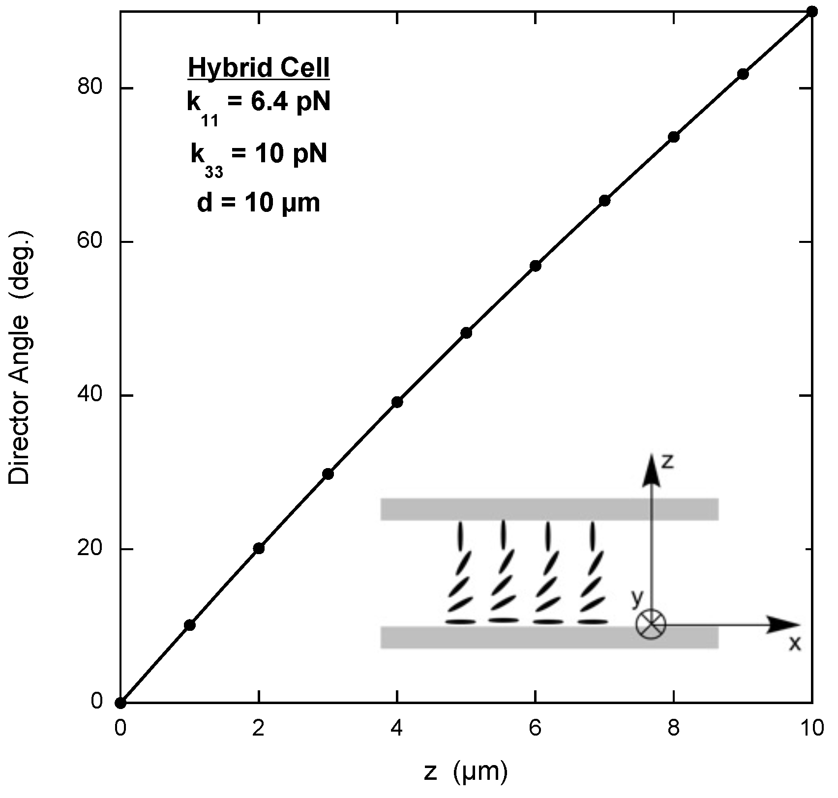
Figure 1 shows a plot of the GA solution with the lowest free energy after 25 iterations. The exact solution, which is found by writing in terms of the angle between the director and the x-axis and then solving the corresponding Euler equation numerically, is also shown [17]. The agreement is excellent.
3.2. Frederiks Transition
The Frederiks transition occurs when a uniformly oriented nematic LC between two parallel substrates is perturbed by an applied electric field. In one geometry, the director is parallel to the x-axis at both substrates with infinite anchoring strength and the electric field is applied along the z-axis (see the inset of Figure 2). Up to a critical value of the electric field, there is no perturbation of the director. However, as the field increases above this value, the director begins to rotate toward the z-axis, first in the middle of the cell and with higher field extending toward the substrates. As for the hybrid cell, , so the bulk elastic free energy density given in Equation (4) applies. However, the electric field term, Equation (3), must be included with , where V is the voltage applied across the cell and d is the distance between the substrates. This means that the calculation of the free energy density must determine in order to compute the integral. A typical script is shown on page 4 of the Supplementary Materials. The parameter “factor” in the script is just (with =11) and the only change to the GA script is to specify a crossover fraction of 0.8.
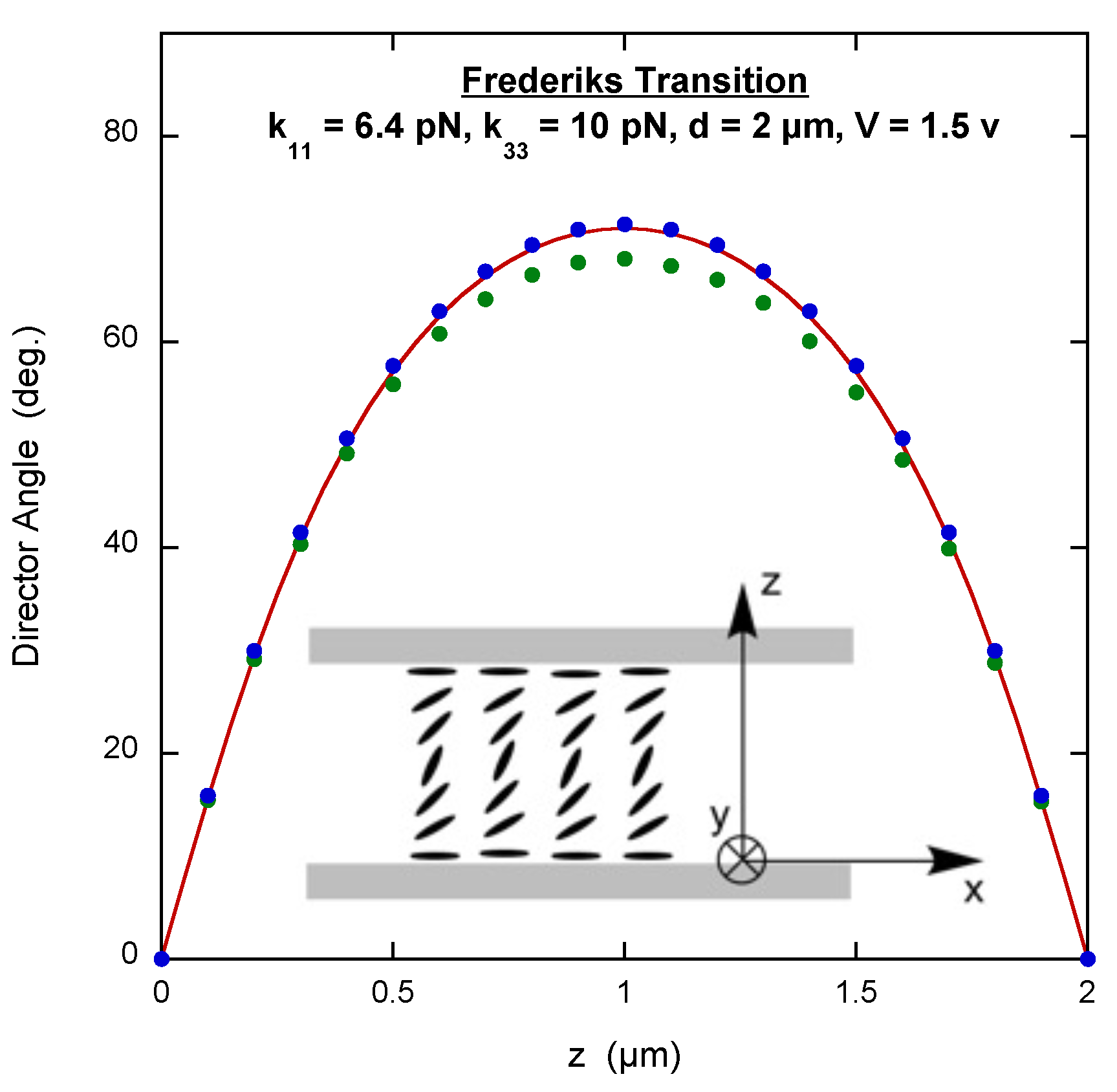
Figure 2 displays the results along with the exact solution, which is also found by writing in terms of the angle between the director and the x-axis and then solving the corresponding Euler equation numerically [17]. Notice that the results do not correspond extremely well to the exact solution. This is an example of what can happen when the number of calculation points increases. Interestingly, the results do not improve if constraints are placed on the values specifying that they are symmetric about the middle of the cell.
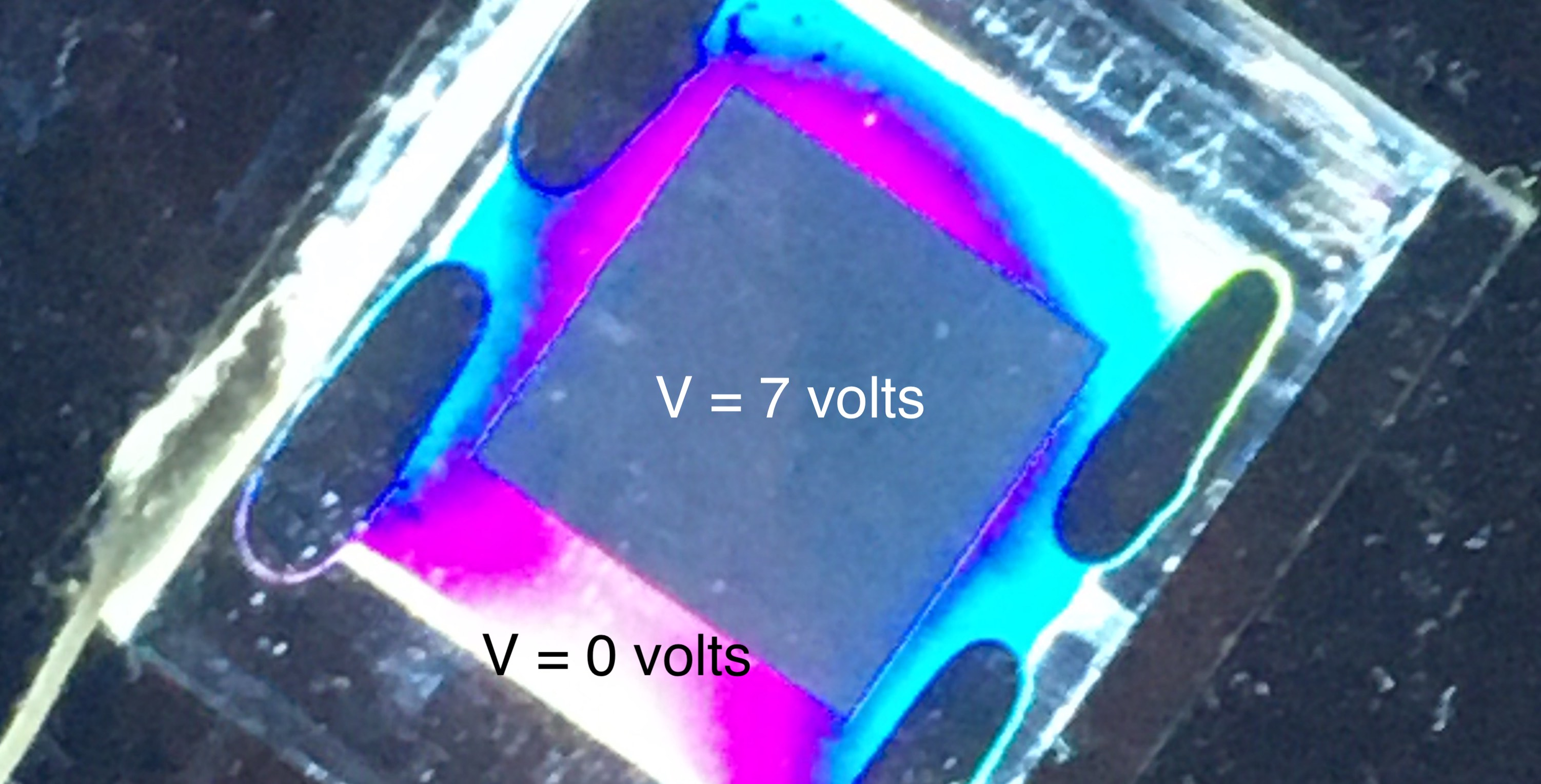
The Frederiks transition is illustrated in the Graphical Abstract. The cell is between crossed polarizers with the director oriented in the plane of the cell at 45 to the polarizers. This causes optical retardation and light emerges from the cell. When a voltage much higher than the threshold voltage is applied, the director orients perpendicular to the substrates, causing the optical retardation to become very small. Therefore, little light exits the cell.
What does increase the accuracy is a script that solves for the values for only half the cell, and the other half of the values are symmetrically equated to them. In this case only the fact that is used in the calculation, i.e., n_x_b = [1 n_x]. Such a GA script is on page 4 of the Supplementary Materials. The results obtained for this script are also shown in Figure 2, where it is clear that they correspond more closely to the exact solution.
3.3. 90-Degree Twist Cell
In a 90 twist cell, the bottom substrate has been prepared to align the director along the x-axis and the top substrate has been prepared to align the director along the y-axis (see inset in Figure 3). To make the situation more realistic, the anchoring strength of the alignment at the substrate surfaces is set to be finite. This means that the free energy density to be minimized must contain the surface expression of Equation (2) along with the volume elastic free energy density of Equation (1).
In this case the director has x- and y-components that only depend on the position along the z-axis, i.e., . Substituting into Equation (1) reveals that there is no splay deformation,
Given the situation, it is difficult to imagine the presence of bend deformation. This can be checked by letting and , where is the angle the director makes with the x-axis in the xy-plane. Substituting this into Equation (5) results in the twist term becoming and the bend term equalling zero. This points out the fact that often the free energy density can be expressed more simply in terms of another parameter instead of the director components. In the interest of uniformity, all GA scripts use the director components, yielding the following for the total free energy density (energy per unit area) for the 90 twist cell.
The symmetry of the situation demands that . Interestingly, specifying this constraint in the GA makes the script run slower and does not improve the accuracy of the results.
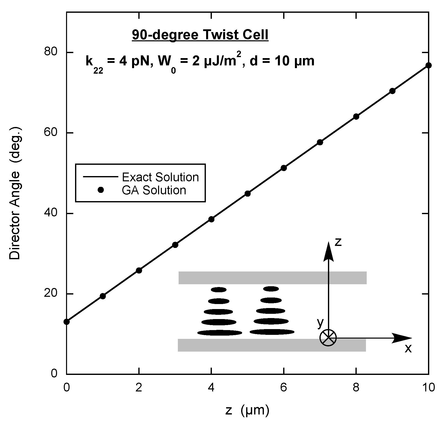
An example of the energy script is on page 5 of the Supplementary Materials. The results are shown in Figure 3, along with the exact solution, which is again found by writing in terms of the angle between the director and the x-axis and then solving the corresponding Euler equation numerically [18]. As with the hybrid cell, the agreement is excellent.
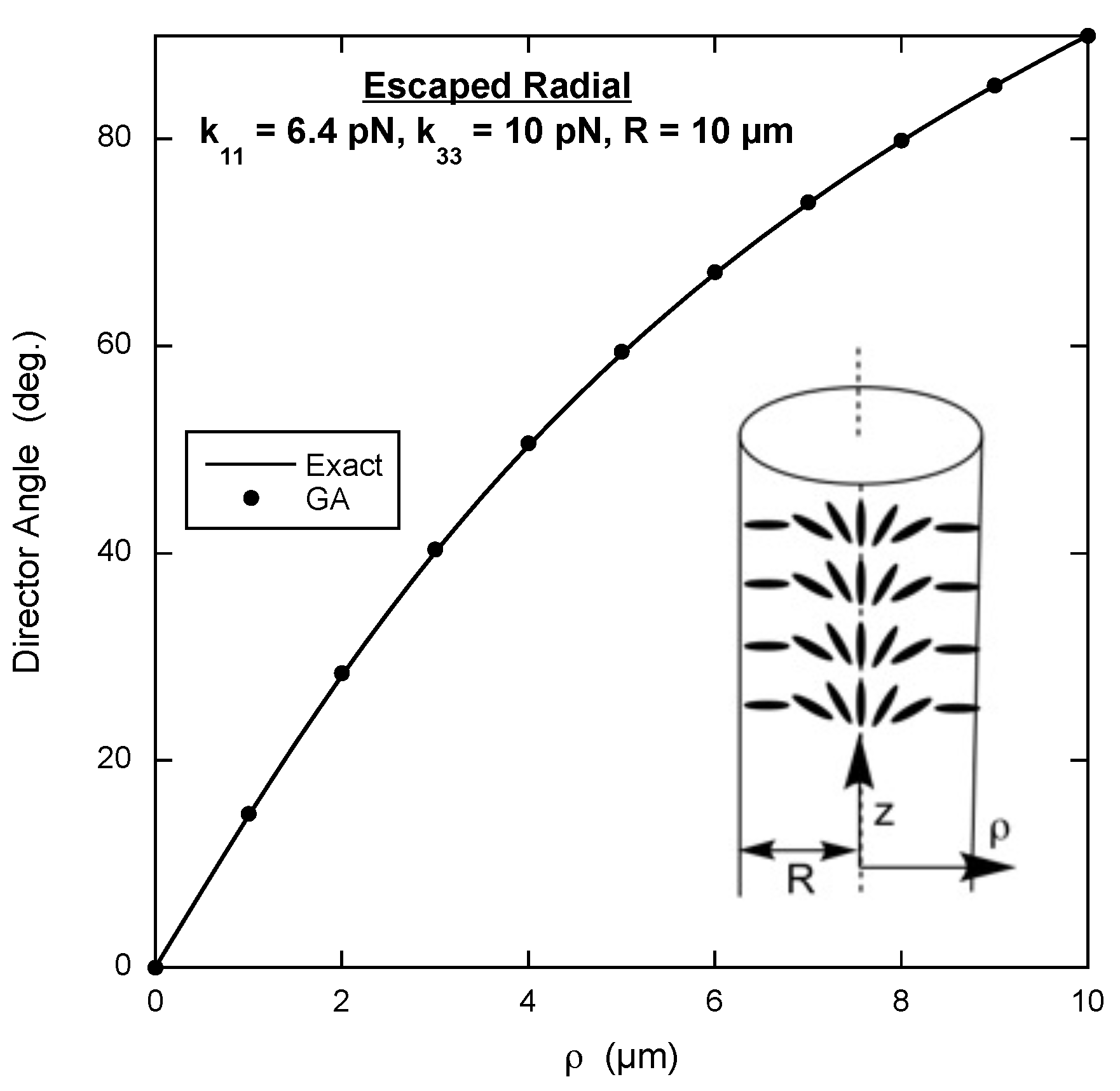
3.4. Escaped Radial Configuration
An interesting example for the genetic algorithm to solve is the director configuration inside a cylinder with the director constrained to be perpendicular to the inner surface. If the bend elastic constant is not too large, the director adopts what is called the escaped radial configuration. Along the central axis of the cylinder, the director is parallel to the axis, and as the director gets closer to the inside boundary of the cylinder, the angle between the director and the cylinder axis increases, reaching 90 at the inner surface. The inset in Figure 4 shows the escaped radial configuration.
It is best to use cylindrical coordinates with the z-axis along the central cylinder axis and the radial axis extending out from the central axis to R, the radius of the inner boundary. Thus there are two non-zero components of the director and both depend on , i.e., . Taking the divergence and curl in cylindrical coordinates reveals there is no twist deformation, yielding the volume free energy density
This volume free energy density must be integrated over the cross-section of the cylinder, which in this case means a differential surface element , where is the angular coordinate of the cylindrical coordinate system. Integrating from 0 to 2 is not done because with no dependence on , it yields a constant that does not affect finding the minimum free energy. However, the integral over must include the factor of from . So the script for the free energy calculation is slightly different (see page 5 of the Supplementary Materials).
The exact solution is once more found by numerically solving the Euler equation that comes from minimizing the free energy density expression written in terms of the angle the director makes with the cylinder’s central axis [19]. The result of the genetic algorithm and the exact solution are displayed in Figure 4. In spite of evaluating the free energy density at only nine points along the radius, the agreement is extremely good.
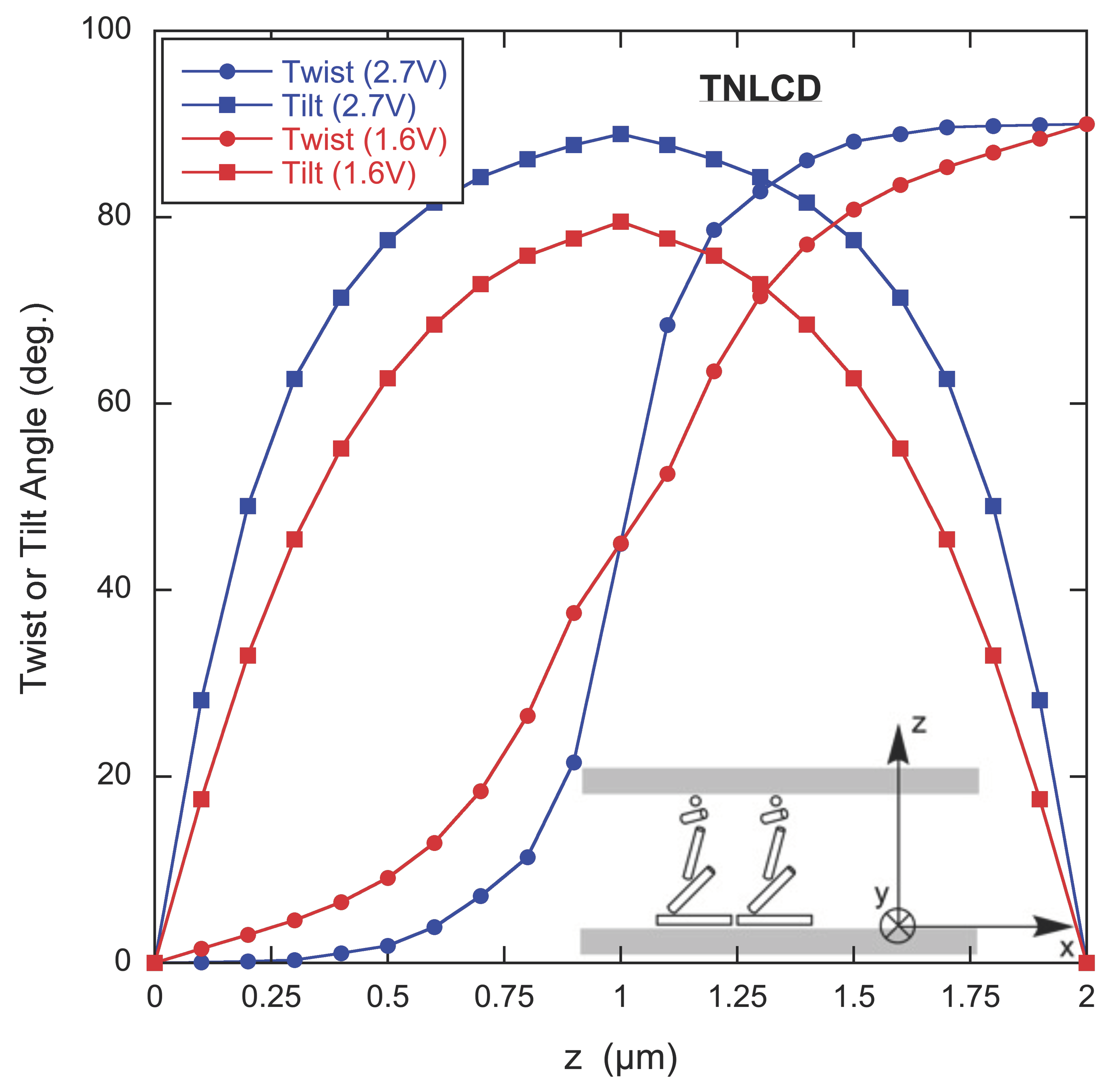
3.5. Twisted Nematic (TN) Cell
The twisted nematic (TN) liquid crystal display was the most successful of the early LCDs. The substrates are prepared to produce a 90 twist cell with a polarizer on each substrate parallel to the surface alignment direction. With no voltage applied, the linearly polarized light entering the display follows the director and thus is rotated by 90 when it encounters the other polarizer, therefore passing through. With either a backlight or a reflector, the cell appears bright or silver-colored in the “off” state. When a voltage over the threshold value is applied using transparent electrodes on each substrate, the director in most of the cell aligns perpendicular to the substrates (see the inset in Figure 5). With the light path mostly parallel to the director, there is little change to the entering polarization and most of the light is extinguished by the second polarizer. Thus the display appears dark in its “on” state.
Because all three components of the director are non-zero, i.e., , the expression for the volume free energy density is more complicated,
Again, the symmetry of the director around the mid-plane of the cell means the director for only one-half of the z-axis needs to be determined. However, there are two unknowns for each undetermined director, and , so if there are 10 calculation points, there are 20 unknowns for the GA to find. The value of does not have to be treated as an unknown since the magnitude of the director is 1. So besides the more complicated free energy expression, the scripts must keep track of which unknowns are and which are . Such a script is on page 6 of the Supplementary Materials.
The doubling of the number of independent unknowns also means the above-threshold TN LCD is a challenge for the genetic algorithm to solve. Even when solving only half the cell, it has difficulty finding the global minimum. This difficulty can be avoided by putting constraints on the solution. For example, it can be stipulated that (1) is less than 1, (2) that decreases monotonically and increases monotonically with increasing z, (3) that increases monotonically with increasing z, and (4) that and at the mid-plane of the cell are equal (see page 6 of the Supplementary Materials).
The results of the GA for two voltages are shown in Figure 5. The twist angle is the angle between the projection of the director in the x-y plane and the x-axis. The tilt angle is the angle between the director and the x-y plane. The twist angle goes from 0 to 90 and the tilt angle reaches a maximum at the mid-plane of the cell. How much of the change in the twist angle occurs near the middle of the cell and for how much of the cell the tilt angle is large depends on the applied voltage.
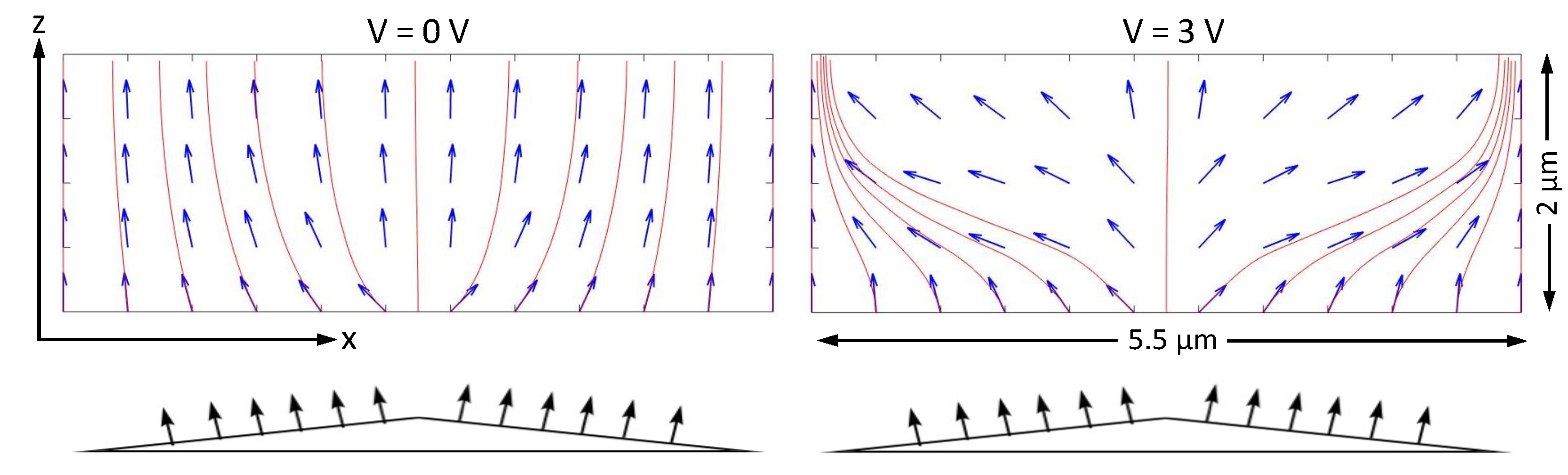
3.6. Vertically Aligned Nematic (VAN) Cell
Can the genetic algorithm handle a situation in which the director depends on two dimensions rather than one? A good example is a vertically aligned nematic (VAN) display cell in which one surface has been treated so the alignment of the director is not uniform. In the most simple VAN display, both substrates have been treated to align the director perpendicular to the substrate. This causes a uniform director configuration throughout the cell. If the liquid crystal has negative dielectric anisotropy, application of an electric field perpendicular to the substrates causes the director to tilt away from its field-free direction. In principle, the tilt can be in any plane perpendicular to the substrates. To make a display with uniform angular viewing, each pixel is engineered so that the tilt is in different planes in different regions. This can be done by adding protruding structures, perhaps small wedges, with a perpendicular alignment layer on them (illustrated at the bottom of Figure 6). In this example, to create the effect of such a double wedge, it is assumed that the bottom surface is flat but prepared so the angle of the director next to the surface varies along the x-axis. Most important, the values of on the bottom surface have opposite signs in the left and right portions of the cell.
For this case, the director can have both an x- and z-component, but both of these components depend on both the x- and z-coordinates, . Substituting into Equation (1) gives
where again it is noted that there is no twist deformation. As before, the electric field term, Equation (3), must be included with , where V is the voltage applied across the cell and d is the distance between the substrates. is negative.
Implementation of the genetic algorithm in this case is a bit more complicated in that the value of must be calculated at points throughout the x-z plane. In the following example, a 3 × 10 grid of 30 calculation points are used (3 perpendicular to the substrates times 10 parallel to the substrates). In addition, is fixed at points one row or column outside the grid of 30 points, with on the sides and top substrate of the cell and varying along the bottom substrate to mimic a two-sided wedge. Thirty values are determined by the GA procedure and thirty values are computed from them, with the free energy script using both to calculate an average value of the four partial derivatives in Equation (9) for each square formed by the grid of calculation points. For example, to calculate , the changes in on the two sides of a grid square parallel to the z-axis are averaged. The average of the four values of at the corners of a grid square is also calculated so that the electric part of the free energy can be included.
In Figure 6, the results of the GA are shown using a two-dimensional vector field and streamlines. When the applied voltage is zero, the alignment condition on the bottom substrate succeeds in slightly tilting the director on each side of the cell in opposite directions. This serves to ensure that when a voltage is applied, the director continues to tilt as desired. When running the GA for cases where the voltage is non-zero, it takes longer and often results in wildly varying solutions. There are so many ways to arrange the director, especially in the central portion of the cell, without much change in the total free energy. Solutions with wildly varying directors occur, usually with much higher free energies, but sometimes with free energies not far from the minimum. Putting in a constraint helps significantly, for example, stipulating that at the six points on either side of the center of the cell must be negative for the three points on the left and positive for the three points on the right.
4. Discussion
The genetic algorithm works quite well in determining director configurations given the very simple nature of the procedure and the fact that no trial solution is required. This includes cases in which surface anchoring and electric field effects are present in addition to the elastic energy considerations. It certainly does not replace the need for sophisticated and much more accurate computational methods in many cases, but it does allow for legitimate calculations with only a shallow learning curve. The presented examples employ a simple implementation of the GA, including the most simple method for performing the integral necessary to compute the free energy. Improvements are certainly possible, but this would bring with it a longer running time than the tens of seconds of the simple routines described here.
Still, there are some considerations that should be taken into account when using the GA in this simple form. Even with about 10 calculation points, the GA often exits without reaching the global minimum free energy. However, this can be overcome by iterating the GA multiple times seeking the lowest free energy. Because the integral method is a simple one, it does best when the director components vary monotonically and close to linearly. When this is not the case, the proportion of incorrect solutions increases and more care is needed when running the routine. The optimal crossover fraction needs to be investigated for each specific case. As one might expect, the easier it is for the GA to find the global minimum, the less necessary it is to use a high crossover fraction. Putting constraints on the solution seems to help only in situations in which there are many sets of director components with about the same free energy. Stipulating smaller tolerance values does not improve the GA much for these types of calculations.
The finding that adding additional calculation points does not improve the solution is interesting. The reason may lie in the fact that the GA works by random procedures rather than following a directed path to the solution. Adding additional points in some senses increases the probability of solutions “wandering” over a larger set of solutions. If the GA cannot discriminate between the many solutions with close-to-minimum free energy, then it may exit with any one of them. This type of difficulty is an active area of research among those who specialize in computational schemes such as neural networks and machine learning. It may resemble the “overfitting” problem in which algorithms are more sensitive to minor variations, perhaps noise, than global aspects of the solution [20]. After all, using the minimization of the free energy as computed by an integral involving derivatives between computation points is not very specific. The GA may work to minimize the contributions to the free energy from small variations among the computation points rather than seeking a wider range of solutions. Researchers have found methods to reduce these types of problems and they certainly can be applied to the presented examples, but that is beyond the subject of this article.
Reference 14 gives a general summary of the strengths and weaknesses of genetic algorithms that seems appropriate when using it to find director configurations.
They are at their best when exploring complex landscapes to locate regions of enhanced opportunity. However, if a partial solution can be improved further by making small changes in a few variables, it is best to augment the generic algorithm with other, more standard methods.
So perhaps the way to use the GA in a research investigation is to produce a first look at the director configuration in a completely unknown situation. If a more precise solution is required, other methods can start with the GA result.
5. Conclusions
The genetic algorithm is a computational technique that is likely to agree with Noel Clark’s sensibilities. It is based on biological heredity, possiblly due to the properties of DNA, one of his favorite building blocks of liquid crystal phases. Using the GA is simple, and once a short script has been written to compute the free energy, very different situations can be solved easily and quickly. With this simplicity comes some drawbacks. However, they are easily understood and in many cases can be solved. In short, the genetic algorithm allows researchers and students to get a glimpse of the behavior of confined liquid crystals without a great deal of work.
Supplementary Materials
The following are available online at https://0-www-mdpi-com.brum.beds.ac.uk/2073-4352/10/11/1041/s1, Table S1: Definition of Variables Used in the Genetic Algorithm Codes. Examples of Genetic Algorithm Codes.
Author Contributions
Both authors contributed to most aspects of the project, including conceptualization, methodology, software, validation, formal analysis, investigation, and writing (reviewing and editing). P.J.C. supervised the project and wrote the original draft. All authors have read and agreed to the published version of the manuscript.
Funding
This research received no external funding.
Acknowledgments
The authors thank Amy Graves for helpful discussions.
Conflicts of Interest
The authors declare no conflict of interest.
Abbreviations
The following abbreviations are used in this manuscript:
| LC | liquid crystal |
| LCD | liquid crystal display |
| GA | genetic algorithm |
| 5CB | 4-cyano-4’-pentylbiphenyl |
References
- Nakata, M.; Zanchetta, G.; Chapman, B.D.; Jones, C.D.; Cross, J.O.; Pindak, R.; Bellini, T.; Clark, N.A. End-to-end stacking and liquid crystal condensation of 6– to 20–base pair DNA duplexes. Science 2007, 318, 1276–1279. [Google Scholar] [CrossRef] [PubMed]
- Zanchetta, G.; Nakata, M.; Buscaglia, M.; Clark, N.A.; Bellini, T. Liquid crystal ordering of DNA and RNA oligomers with partially overlapping sequences. J. Phys. Condens. Matter 2008, 20, 494214-1–494214-6. [Google Scholar] [CrossRef]
- Zanchetta, G.; Giavazzia, F.; Nakata, M.; Buscaglia, M.; Cerbino, C.; Clark, N.A.; Bellini, T. Right-handed double-helix ultrashort DNA yields chiral nematic phases with both right- and left-handed director twist. Proc. Natl. Acad. Sci. USA 2010, 107, 17479–417502. [Google Scholar] [CrossRef] [PubMed] [Green Version]
- Bellini, T.; Zanchetta, G.; Fraccia, T.P.; Cerbino, R.; Tsai, E.; Smith, G.P.; Moran, M.J.; Walba, D.M.; Clark, N.A. Liquid crystal self-assembly of random- sequence DNA oligomers. Proc. Natl. Acad. Sci. USA 2010, 109, 1110–1115. [Google Scholar] [CrossRef] [PubMed] [Green Version]
- Yoon, D.K.; Smith, G.P.; Tsai, E.; Moran, M.; Walba, D.M.; Bellini, T.; Smalyukh, I.I.; Clark, N.A. Alignment of the columnar liquid crystal phase of nano-DNA by confinement in channels. Liq. Cryst. 2012, 39, 571–577. [Google Scholar] [CrossRef]
- Rossi, M.; Zanchetta, G.; Klussmann, S.; Clark, N.A.; Bellini, T. Propagation of Chirality in Mixtures of Natural and Enantiomeric DNA Oligomers. Phys. Rev. Lett. 2013, 110, 107801-1–107801-5. [Google Scholar] [CrossRef] [PubMed] [Green Version]
- Fraccia, T.P.; Smith, G.P.; Zanchetta, G.; Paraboschi, E.; Yi, Y.; Walba, D.M.; Dieci, G.; Clark, N.A.; Bellini, T. Abiotic ligation of DNA oligomers templated by their liquid crystal ordering. Nat. Commun. 2015, 6, 6424. [Google Scholar] [CrossRef] [PubMed] [Green Version]
- Liu, K.; Shuai, M.; Chen, D.; Tuchband, M.; Gerasimov, J.Y.; Su, J.; Liu, Q.; Zajaczkowski, W.; Pisula, W.; Müllen, K.; et al. Solvent-free Liquid Crystals and Liquids from DNA. Chem. Eur. J. 2015, 21, 4898–4903. [Google Scholar] [CrossRef] [PubMed]
- Fraccia, T.P.; Smith, G.P.; Bethge, L.; Zanchetta, G.; Nava, G.; Klussmann, S.; Clark, N.A.; Bellini, T. Liquid Crystal Ordering and Isotropic Gelation in Solutions of Four-Base-Long DNA Oligomers. ACS Nano 2016, 10, 8508–8516. [Google Scholar] [CrossRef] [PubMed]
- Saurabh, S.; Lansac, Y.; Jang, Y.H.; Glaser, M.A.; Clark, N.A.; Maiti, P.K. Understanding the origin of liquid crystal ordering of ultrashort double-stranded DNA. Phys. Rev. E 2017, 95, 032702-1–032702-6. [Google Scholar] [CrossRef] [PubMed] [Green Version]
- Fraccia, T.P.; Smith, G.P.; Clark, N.A.; Bellini, T. Liquid Crystal Ordering of Four-Base-Long DNA Oligomers with Both G–C and A–T Pairing. Crystals 2018, 8, 5. [Google Scholar] [CrossRef] [Green Version]
- Smith, G.P.; Fraccia, T.P.; Todisco, M.; Zanchetta, G.; Zhu, C.; Hayden, E.; Bellini, T.; Clark, N.A. Backbone-free duplex-stacked monomer nucleic acids exhibiting Watson–Crick selectivity. Proc. Natl. Acad. Sci. USA 2018, 115, E7658–E7664. [Google Scholar] [CrossRef] [PubMed] [Green Version]
- Theis, J.G.; Smith, G.P.; Yi, Y.; Walba, D.M.; Clark, N.A. Liquid crystal phase behavior of a DNA dodecamer and the chromonic dye Sunset Yellow. Phys. Rev. E 2018, 98, 042701-1–042701-6. [Google Scholar] [CrossRef] [Green Version]
- Holland, J.H. Genetic algorithms. Sci. Am. 1992, 267, 66–72. [Google Scholar] [CrossRef]
- Sutton, P.; Boyden, S. Genetic algorithms: A general search procedure. Am. J. Phys. 1994, 62, 549–552. [Google Scholar] [CrossRef]
- Kern, S.; Muller, S.D.; Hansen, N.; Buche, D.; Ocenasek, J.; Koumoutsakos, P. Learning probability distributions in continuous evolutionary algorithms—A comparative review. Nat. Comput. 2004, 3, 77–112. [Google Scholar] [CrossRef]
- Collings, P.J.; Goodby, J.W. Introduction to Liquid Crystals: Chemistry and Physics, 2nd ed.; Taylor & Francis Group: Boca Raton, FL, USA, 2020; p. 418. [Google Scholar]
- McGinn, C.K.; Laderman, L.I.; Zimmermann, N.; Kitzerow, H.-S.; Collings, P.J. Planar anchoring strength and pitch measurements in achiral and chiral chromonic liquid crystals using 90-degree twist cells. Phys. Rev. E 2013, 88, 062513-1–062513-9. [Google Scholar] [CrossRef] [PubMed] [Green Version]
- Crawford, G.P.; Allender, D.W.; Doane, J.W. Surface elastic and molecular anchoring properties of nematic liquid crystals confined to cylindrical cavities. Phys. Rev. A 1992, 45, 8693–8708. [Google Scholar] [CrossRef] [PubMed] [Green Version]
- Massaron, L.; Boschetti, A. Regression Analysis with Python; Packt Publishing Ltd.: Birmingham, UK, 2016. [Google Scholar]
Figure 1.
Director angle in a hybrid cell with infinite anchoring strength. Inset: schematic of a hybrid cell. The director angle is measured from the x-axis. Solid circles: genetic algorithm results. Solid line: exact solution.
Figure 1.
Director angle in a hybrid cell with infinite anchoring strength. Inset: schematic of a hybrid cell. The director angle is measured from the x-axis. Solid circles: genetic algorithm results. Solid line: exact solution.

Figure 2.
Director angle for the Frederiks transition with and infinite anchoring strength. Inset: schematic of the cell. The director angle is measured from the x-axis. Green circles: genetic algorithm results for 19 calculation points across the entire cell. Blue circles: genetic algorithm results for 10 calculation points across half the cell. Red line: exact solution.

Figure 3.
Director angle for the 90-degree twist cell. Inset: schematic of the cell. The director angle is measured from the x-axis in the xy-plane. Black circles: genetic algorithm results; black line: exact solution.
Figure 3.
Director angle for the 90-degree twist cell. Inset: schematic of the cell. The director angle is measured from the x-axis in the xy-plane. Black circles: genetic algorithm results; black line: exact solution.

Figure 4.
Director angle for the escaped radial director configuration in a cylinder. Inset: schematic of the cylinder. The director angle is measured from the z-axis in the z-plane. Black circles: genetic algorithm results; black line: exact solution.
Figure 4.
Director angle for the escaped radial director configuration in a cylinder. Inset: schematic of the cylinder. The director angle is measured from the z-axis in the z-plane. Black circles: genetic algorithm results; black line: exact solution.

Figure 5.
Twist and tilt director angles for the twisted nematic LCD at two different voltages using the genetic algorithm ( = 6.4 pN, = 4.0 pN, pN, d = 2 m). Inset: schematic of the cell. The twist angle is measured from the x-axis in the xy-plane. The tilt angle is measured perpendicularly from the xy-plane.

Figure 6.
Director angle in a vertically aligned nematic (VAN) display with protrusions to produce opposite tilt directions in the two halves of the cell ( = 6.4 pN, = 10 pN, d = 2 m, = −3). As explained in the text, the boundary conditions on the bottom substrate mimic a small protruding two-sided wedge with perpendicular anchoring, an example of which is illustrated just below the cell. The boundary condition on the other three sides is = 0 (not shown on the top substrate).

Publisher’s Note: MDPI stays neutral with regard to jurisdictional claims in published maps and institutional affiliations. |
© 2020 by the authors. Licensee MDPI, Basel, Switzerland. This article is an open access article distributed under the terms and conditions of the Creative Commons Attribution (CC BY) license (http://creativecommons.org/licenses/by/4.0/).
Share and Cite
MDPI and ACS Style
Yang, S.; Collings, P.J. The Genetic Algorithm: Using Biology to Compute Liquid Crystal Director Configurations. Crystals 2020, 10, 1041. https://0-doi-org.brum.beds.ac.uk/10.3390/cryst10111041
AMA Style
Yang S, Collings PJ. The Genetic Algorithm: Using Biology to Compute Liquid Crystal Director Configurations. Crystals. 2020; 10(11):1041. https://0-doi-org.brum.beds.ac.uk/10.3390/cryst10111041
Chicago/Turabian StyleYang, S., and Peter J. Collings. 2020. "The Genetic Algorithm: Using Biology to Compute Liquid Crystal Director Configurations" Crystals 10, no. 11: 1041. https://0-doi-org.brum.beds.ac.uk/10.3390/cryst10111041
Note that from the first issue of 2016, this journal uses article numbers instead of page numbers. See further details here.