
Modeling of the Resonant X-ray Response of a Chiral Cubic Phase


1
Department of Physics, Faculty of Natural Sciences and Mathematics, University of Maribor, Koroška 160, 2000 Maribor, Slovenia
2
Faculty of Chemistry, University of Warsaw, Żwirki i Wigury 101, 02-089 Warsaw, Poland
3
Jozef Stefan Institute, Jamova 39, 1000 Ljubljana, Slovenia
*
Author to whom correspondence should be addressed.
Crystals 2021, 11(2), 214; https://0-doi-org.brum.beds.ac.uk/10.3390/cryst11020214
Submission received: 2 February 2021
/
Revised: 15 February 2021
/
Accepted: 18 February 2021
/
Published: 21 February 2021
(This article belongs to the Special Issue In Celebration of Noel A. Clark’s 80th Birthday)
Abstract
:The structure of a continuous-grid chiral cubic phase made of achiral constituent molecules is a hot topic in the field of thermotropic liquid crystals. Several structural models have been proposed so far. Resonant X-ray scattering (RXS), which gives information on the molecular orientation in the unit cell, could be applied to select the most appropriate model. We modeled the RXS response for the recently proposed chiral cubic phase structure with an all-hexagon chiral continuous grid. A tensor form factor of a unit cell is constructed, which enables calculation of intensities of peaks for all Miller indices. We find that all the symmetry allowed peaks are resonantly enhanced, and their intensity is much stronger than the intensity of the symmetry forbidden (resonant) peaks. In particular, we predict that a strong resonant enhancement of the symmetry allowed peaks (011) and (002), not observed in a nonresonant scattering, could be observed by RXS at the carbon absorption edge. By RXS at the sulfur absorption edge, one might observe a resonant peak (113) and resonantly enhanced peak (233), and resonant enhancement of all the peaks that are observed in a nonresonant scattering, which probably hide the rest of the predicted resonant peaks.
1. Introduction
Organization of molecules in three-dimensional continuous channel network in thermotropic liquid crystals has attracted much interest from two points of view. The first is their complexity; these phases are interesting from a basic research point of view. The second one is their potential for applications as optical materials [1], mechanically resistant materials [2] and in photovoltaics [3]. The unit cells of these phases are extremely large: the length of the unit cell is of the order of 10 nm, and the cell contains several thousand molecules. Especially interesting is a chiral cubic phase, the structure of which is still under debate. Upon the first observations of the phase [4,5], its chirality was not recognized and the phase was assigned the achiral symmetry. Two structural models were proposed for the phase. A three-continuous-grid model [6] with continuous grids of channels, two of them consisting of interconnected octagons and the one between them of interconnected hexagons. In a one-continuous-grid model [7], the octagons were replaced by micelles that are enclosed by a continuous grid formed by interconnected hexagons. Neither of these models could reproduce well the intensities of the peaks observed in the X-ray scattering studies, especially regarding the intensities of the two most intensive peaks with Miller indices and . Almost a decade after the first observation of the cubic phase with the symmetry (assigned at that time), chiral domains were observed in this phase [8]. The symmetry still persists in referring to this phase, but quote marks are usually added (“”) to point out that the symmetry is not proper for this phase. We will refer to this phase as a chiral cubic () phase, instead.
Several models were proposed so far to explain the origin of chirality in the chiral cubic phase [8,9,10,11]. The latest two models [10,11] were proposed in 2020. Zeng and Ungar constructed a three-continuous-grid with the symmetry [10]. This model requires a significant rearrangement of molecules upon the transition from/to the cubic phase with the symmetry having a double gyroid structure [12] of channels. The cubic phase, which is often observed in a sequence with the CC phase, is built of two intertwining continuous grids (bicontinuous phase) of opposite chirality (Figure 1) and a helical arrangement of long molecular axes along the channels [8,13,14,15]. Because the phase transition from the double gyroid phase to the chiral cubic phase occurs with a negligible enthalpy change [16], such an extensive rearrangement of molecules as required by the channel arrangement in the phase with the symmetry is less probable. In addition, the proposed structure with the symmetry does not give the peak as the second highest intensity peak in the X-ray scattering studies. Another model, presented in Reference [11], is based on the one-continuous-grid model with micelles; however, the lengths of the hexagon sides are matched to the lengths of the channels in the lower or upper temperature double gyroid phase and the direct connections among the hexagons are replaced by channels connected to the unit cell edges or faces, as shown in Figure 1. This model predicts proper intensity ratios among the highest intensity peaks in the X-ray scattering. The basic idea behind the model is that the structure of channels in the continuous grid (i.e., the major electron density) retains the symmetry; however, the molecules on the opposite sides of the hexagon are slightly tilted up/down in order to give more space for flexible aliphatic chains. Because each hexagon is nonplanar (it has an armchair geometry, see Figure 2), the mirror symmetry is broken. The packing of the eight hexagons in the unit cell can be chiral or achiral, but having all the hexagons of the same chirality leads to more space for aliphatic tails also among the molecules in the neighboring hexagons; thus, the chirality propagates from one hexagon to the unit cell and to the whole phase [11].
Which of the proposed models (if any) of the chiral cubic phase is a proper one could be determined by the resonant X-ray studies. In this paper, we develop a method by which one can predict the intensity of the resonant and resonantly enhanced peaks that are expected for the structure of the chiral cubic phase proposed in Reference [11]. The model presented also gives a general approach to the prediction of the positions and intensities of the resonant and resonantly enhanced peaks for the other proposed structures. By comparing predictions to experimental measurements, once they are available, one could thus decide on the proper structure of the chiral cubic phase. This approach has recently proven successful to determine the structure of the double gyroid phase [15].
2. Methods
To determine molecular orientation in addition to the periodic electron density variation, resonant X-ray scattering (RXS) is used. When the energy of the incident photons is close to the absorption edge of some element present in the material (sulfur and carbon are usually used), the form factor of the material investigated becomes anisotropic; it becomes a tensor quantity, while it is a scalar for a nonresonant X-ray scattering. As a result, one can obtain scattering peaks at positions that are forbidden by the symmetry of the phase [17,18,19] (resonant peaks), as well as enhancement in the intensity of the symmetry allowed peaks (resonantly enhanced peaks) [18,20]. Because the form factor is a tensor quantity, the intensity of the peaks depends on the polarization of the incident X-rays [20,21]. The theoretical basis for the description of the RXS in liquid crystals was given by B. Pansu in A. M. Levelut [22], who suggested that the form factor is analogous to the anisotropic part of the polarizability tensor. In order to calculate the position and intensity of the resonant and resonantly enhanced peaks, one thus has to obtain the tensor form factor first and evaluate it at the values of the Miller indices allowed by the cubic symmetry (). The intensity of a chosen peak with the Miller indices depends on the scattering amplitude (), which is calculated from the tensor form factor as [17]:
where and are polarization directions of the incident and scattered wave, respectively. The polarization direction of the incident and scattered wave is split into a component perpendicular to the scattering plane (-polarization) and a component lying in the scattering plane (-polarization). Based on the polarization of the incident and scattered wave, four scattering amplitudes , , and are defined, where the first index denotes the polarization of the scattered wave and the second one the polarization of the incident wave [17]:
If unpolarized light is used in the measurements and no polarization grating is used to filter the output light, the intensity of the scattered light () is calculated as a sum of squares of scattering amplitudes of all possible pairs of polarizations:
3. Results
In this section we present the construction of the model, calculation of the tensor form factor and intensities of the resonant and resonantly enhanced peaks. In the case of the resonantly enhanced peaks, we focus only on the peaks that are allowed by the symmetry but are not observed in the nonresonant X-ray scattering.
3.1. Tensor Form Factor
To calculate the tensor form factor of the unit cell, we use a simplified model of the unit cell. We assume that the major contribution to the RXS response is due to a slight up/down shift of the molecules on the neighboring sides of nonplanar hexagons (blue hexagons in Figure 1b). Next, a group of molecules that are arranged along the channels presented by the hexagon sides is replaced by a single anisotropic scatterer placed in the midpoint of a hexagon side. We assume that the polarizability of this scatterer in the direction of the molecular long axis (we shall call it the polarization axis, blue and red lines in Figure 2; Figure 3) is different than perpendicular to it. We calculate the tensor form factor of the unit cell as a sum of the tensor form factors of all individual scatterers (six on each hexagon, eight hexagons in the unit cell, see Figure 3).
We begin by examining scatterers on one of the hexagons and calculate the tensor form factor in the coordinate system centered in the hexagon (Figure 2). The length of the hexagon side within this model is , where is the length of the side of the unit cell [11]. Positions of scatterers and orientation of their polarization axes in the case of are given in Table 1.
We assume that the tensor form factor of one anisotropic scatterer is proportional to the anisotropic part of the polarizability tensor. In the eigen system in which the axis points along the direction of the long molecular axis, i.e., along the polarization axis, the tensor form factor () of a single anisotropic scatterer is equal to:
where is the tensor element.
In order to obtain the tensor form factor of the unit cell in the laboratory system, in which the direction of axes , and are along the sides of the unit cell (Figure 3), we first rotate the tensor form factor of one scatterer from the eigen system to the coordinate system centered on the hexagon as follows. The unit vector , given in Table 1, is rotated by the rotation matrix by an angle around the hexagon side to account for the polarization axes of the scatterers on the opposite sides of the hexagons, tilted such that the hexagon is chiral. This unit vector is then rotated by the rotation matrix to point along the axis of the eigen system:
The tensor form factor of the -th anisotropic scatterer in the coordinate system of the hexagon () is then:
There is a single anisotropic scatterer on each side of each hexagon, so we obtain the tensor form factor () of a single hexagon in the coordinate system of the hexagon (Figure 2) by summing up the tensor form factors of all the scatterers, including the phase difference between them due to their different positions on the hexagon:
where is the scattering vector expressed in the coordinate system of the hexagon and is the position of the -th anisotropic scatterer, i.e., the midpoint of the -th side of the hexagon, again given in the coordinate system of the hexagon. The vectors are obtained from the positions of the hexagon’s vertices () (see Table 1) as
The tensor form factor of the unit cell is a sum of the tensor form factors of all the hexagons in the unit cell. Once a single hexagon with the belonging scatterers is defined in the coordinate system centered on the hexagon, we can use translations and rotations to place it in the proper position; the center of each hexagon is in the center of each octant of the unit cell. Orientation of each individual hexagon in the laboratory coordinate system, the origin of which is in the center of the unit cell and the axes run along the unit cell sides, is determined by the directions of axes and , which are given by the unit vectors and . These parameters for our model are presented in Table 2.
As seen from Figure 2, in the coordinate system centered on the hexagon points along the axis, while points along the axis. Thus, we can obtain the rotation matrix , which acts on the unit vector to transform it into in the following way:
In the same way, we define the rotation matrix :
where is the unit vector that points along in the laboratory system. Because vectors and are orthogonal, we obtain the tensor form factor () of the -th hexagon in the laboratory system as:
The tensor form factor of one unit cell is now constructed by summing up the tensor form factors of all the hexagons, taking into account the phase shift due to their relative positions in the unit cell:
where is the position of the center of the -th hexagon inside the unit cell (see Table 2). is the scattering vector in the laboratory system:
where , and are Miller indices. The scattering vector is given in the laboratory system, while the scattering vector in Equation (10) is given in the coordinate system of the hexagon. The relation between them for the -th hexagon is:
3.2. Resonant and Resonantly Enhanced Peaks
By using Equation (15), we can calculate the tensor form factors for any combination of Miller indices (). We find that all the peaks allowed by the symmetry are resonantly enhanced. In addition, the model predicts 10 purely resonant peaks for the combination of Miller indices such that . Because of a cubic symmetry, permutations of Miller indices should only affect the position of the tensor form factor elements without changing their magnitudes. This was used to debug the model. Table 3 gives tensor form factors for the resonant peaks and only those resonantly enhanced peaks that are not observed in a nonresonant X-ray scattering.
3.3. Intensities of the Peaks
Intensities of the resonant and resonantly enhanced peaks are calculated by following the procedure given in Section 2, where in Equations (2)–(5) is from Equation (15) and given explicitly in Table 3, calculated at Miller indices . The polarization directions and are obtained in the following way. Figure 4 shows the scattering plane, which is defined by the scattering vector for the peak with Miller indices () and the wave vector of the incident () and scattered () wave. The angle between the vector and the plane is denoted by , while the angle between and plane is . A projection of the scattering vector on the plane forms an angle with the axis. The components of the incident and scattered wave in the scattering plane ( and ) and perpendicular to it ( and ) are
From Figure 4, we observe that the angle and the angle , where is the angle between the scattering vector and axis and , is the scattering angle for the peak (). From the condition we obtain:
where is the wave number and is the wavelength of the incident X-rays. By using Equations (16) and (22), we find:
In the case of a powder sample, we average the intensity of the peak with Miller indices () over and multiply it by the multiplicity of the peak (). The calculated intensities of the resonant and resonantly enhanced peaks are given in Table 4. Intensities of the peaks , and were calculated with the X-ray wavelength , which corresponds to X-rays at the absorption edge of carbon (resonant soft X–ray scattering, RSoXS). Intensities of the rest of the peaks were calculated with the X-ray wavelength , which corresponds to X-rays at the absorption edge of sulfur (tender resonant X-ray scattering, TReXS). The intensity of the peak () was calculated by using both wavelengths. An intensity of a chosen peak is normalized with respect to the intensity of the peak (), due to the reasons provided in the discussion. Results are given for two inclinations of scatterers: and (see Figure 2).
4. Discussion and Conclusions
We modeled the resonant X–ray scattering response for the structural model of the chiral cubic phase proposed in Reference [12]. This model predicts a one-continuous grid, which is built of molecules arranged into channels that form hexagons with an armchair geometry. The length of one segment in the hexagon is the same as the length of the segments forming a double gyroid structure of the phase, the phase to which CC structure evolves on heating or cooling. Hexagons are connected by lower density channels, as shown in Figure 1. A grid of hexagons surrounds micelles. The model predicts that the chirality of the phase originates from the packing of molecules along the hexagon sides. In order to enable more space for the fluctuation of the aliphatic tails, molecules at the centers of the opposite sides are slightly tilted up/down as shown in Figure 2. The resonant X-ray scattering response was modeled by putting one anisotropic scatterer at the center of each hexagon side, the axis of the largest/lowest polarizability being along the direction of the long molecular axis.
The model predicts that all the symmetry allowed peaks are resonantly enhanced and their intensity is much stronger than the intensity of the pure resonant peaks (see Table 4). One thus expects that all the peaks that are observed in a nonresonant scattering will also be detected in the resonant scattering experiments. Because of that, we plot the resonantly enhanced peaks and resonant peaks on top of the experimental diffractogram [11] obtained by a nonresonant scattering (Figure 5). We plot only those resonantly enhanced peaks that were not observed in the nonresonant scattering: (011), (002) and (233). Concerning the purely resonant peaks, they are all very weak and their positions are close to the resonantly enhanced peaks, except for the peak (113). This is the reason why, in Table 4, we normalized the calculated intensities with respect to the (113) peak. The predicted resonant peaks (023), (223)/(014), (124) and (034) are of a comparable or higher intensity than the (113) peak (Figure 5). However, since they all lie close to the resonantly enhanced peaks, the intensities of which are three orders of magnitude higher than the intensities of the resonant peaks (assuming a small tilt of molecules, ) or one order of magnitude higher if we increase the tilt to , we expect that only the peak (113) might be detectable.
Based on the theoretical modeling, we thus predict that for the structure of the chiral cubic phase proposed in Reference [11], one should observe resonantly enhanced peaks (011) and (002) when using the resonant X-ray scattering at the carbon absorption edge. By the resonant X-ray scattering at the sulfur absorption edge, one might observe the resonant peak (113) and resonantly enhanced peak (233) plus resonantly enhanced all the peaks that are observed in the nonresonant scattering. All the other resonant peaks might be hidden by the nearby resonantly enhanced peaks.
The results reported in this paper can be directly applied to analyze experimental measurements (when these are available) only if powder samples are studied and the incident and scattered beams are not polarized. In the case of polarized incident/scattered light, this should be taken into account in the calculation of the intensity (only the appropriate term in Equation (6) should be taken). In the case of the partially or fully aligned sample, one should omit averaging over and multiplication by the multiplicity factor in the calculation of the intensity. Finally, we point out that the model of the RXS response should also be built for the structural model presented in Reference [10]. Providing that the experimental results will have sufficiently high resolution, it will then be possible to decide if any of the proposed structural models describes well the actual structure of the chiral cubic phase.
Author Contributions
Conceptualization, N.V. and E.G.; model formation, T.G. and N.V.; formal analysis, N.V., E.G., D.P. and T.G.; writing—original draft preparation, T.G. and N.V.; writing—review and editing, N.V., E.G. and D.P.; visualization, T.G. and N.V. All authors have read and agreed to the published version of the manuscript.
Funding
This research was funded by the National Science Center (Poland), grant number 2016/22/A/ST5/00319 and the Slovenian Research Agency (ARRS), through the research core funding no. P1-0055.
Data Availability Statement
Data is contained within the article.
Acknowledgments
E.G. acknowledges funding from the Foundation for Polish Science through the Sabbatical Fellowships Program.
Conflicts of Interest
The authors declare no conflict of interest. The funders had no role in the design of the study; in the collection, analyses, or interpretation of data; in the writing of the manuscript, or in the decision to publish the results.
References
- Dolan, J.A.; Wilts, B.D.; Vignolini, S.; Baumberg, J.J.; Steiner, U.; Wilkinson, T.D. Optical properties of gyroid structured materials: From photonic crystals to metamaterials. Adv. Opt. Mater. 2015, 3, 12–32. [Google Scholar] [CrossRef] [Green Version]
- Pelanconi, M.; Ortona, A. Nature-inspired, ultra-lightweight structures with gyroid cores produced by additive manufacturing and reinforced by unidirectional carbon fiber ribs. Materials 2019, 12, 4134. [Google Scholar] [CrossRef] [Green Version]
- Crossland, E.J.; Kamperman, M.; Nedelcu, M.; Ducati, C.; Wiesner, U.; Smilgies, D.-M.; Toombes, G.E.; Hillmyer, M.A.; Ludwigs, S.; Steiner, U.; et al. A bicontinuous double gyroid hybrid solar cell. Nano Lett. 2009, 9, 2807–2812. [Google Scholar] [CrossRef] [PubMed]
- Kutsumizu, S.; Ichikawa, T.; Nojima, S.; Yano, S. A cubic–cubic phase transition of 4A-n-hexacosyloxy-3A-nitrobiphenyl-4-carboxylic acid (ANBC-26). Chem. Commun. 1999, 1181–1182. [Google Scholar] [CrossRef]
- Imperor-Clerc, M.; Sotta, P.; Veber, M. Crystal shapes of cubic mesophases in pure and mixed carboxylic acids observed by optical microscopy. Liq. Cryst. 2000, 27, 1001–1009. [Google Scholar] [CrossRef]
- Zeng, X.; Ungar, G.; Impéror-Clerc, M. A triple-network tricontinuous cubicliquid crystal. Nat. Mater. 2005, 4, 562–567. [Google Scholar] [CrossRef]
- Ozawa, K.; Yamamura, Y.; Yasuzuka, S.; Mori, H.; Kutsumizu, S.; Saito, K. Coexistence of Two Aggregation Modes in Exotic Liquid-Crystalline Superstructure: Systematic Maximum Entropy Analysis for Cubic Mesogen, 1,2-Bis (4′-n-alkoxybenzoyl) hydrazine [BABH (n)]. J. Phys. Chem. B 2008, 112, 12179–12181. [Google Scholar] [CrossRef] [PubMed]
- Dressel, C.; Liu, F.; Prehm, M.; Zeng, X.; Ungar, G.; Tschierske, C. Dynamic mirror-symmetry breaking in bicontinuous cubic phases. Angew. Chem. Int. Ed. 2014, 53, 13115–13120. [Google Scholar] [CrossRef] [PubMed] [Green Version]
- Saito, K.; Yamamura, Y.; Miwa, Y.; Kutsumizu, S. A structural model of the chiral “Im 3 m” cubic phase. Angew. Chem. Int. Ed. 2016, 18, 3280–3284. [Google Scholar]
- Zeng, X.; Ungar, G. Spontaneously chiral cubic liquid crystal: Three interpenetrating networks with a twist. J. Mater. Chem. C 2020, 8, 5389–5398. [Google Scholar] [CrossRef]
- Vaupotič, N.; Salamończyk, M.; Matraszek, J.; Vogrin, M.; Pociecha, D.; Gorecka, E. New structural model of a chiral cubic liquid crystalline phase. Phys. Chem. Chem. Phys. 2020, 22, 12814–12820. [Google Scholar] [CrossRef] [PubMed]
- Guillon, D.; Skoulios, A. Molecular model for the “smectic D” mesophase. Europhys. Lett. 1987, 3, 79–85. [Google Scholar] [CrossRef]
- Nakazawa, Y.; Yamamura, Y.; Kutsumizu, S.; Saito, K. Molecular mechanism responsible for reentrance to Ia3d gyroid phase in cubic mesogen BABH (n). J. Phys. Soc. Jap. 2012, 81, 094601. [Google Scholar] [CrossRef]
- Tschierske, C.; Ungar, G. Mirror symmetry breaking by chirality synchronisation in liquids and liquid crystals of achiral molecules. ChemPhysChem 2016, 17, 9–26. [Google Scholar] [CrossRef]
- Cao, Y.; Alaasar, M.; Nallapaneni, A.; Salamończyk, M.; Marinko, P.; Gorecka, E.; Tschierske, C.; Liu, F.; Vaupotič, N.; Zhu, C. Molecular Packing in Double Gyroid Cubic Phases Revealed via Resonant Soft X-ray Scattering. Phys. Rev. Lett. E 2020, 125, 027801. [Google Scholar] [CrossRef]
- Matraszek, J.; Pociecha, D.; Vaupotič, N.; Salamończyk, M.; Vogrin, M.; Gorecka, E. Bi-continuous orthorhombic soft matter phase made of polycatenar molecules. Soft Matter 2020, 16, 3882–3885. [Google Scholar] [CrossRef]
- Dmitrienko, V.E. Forbidden reflections due to anisotropic X-ray susceptibility of crystals. Acta Cryst. A 1983, 39, 29–35. [Google Scholar] [CrossRef]
- Dmitrienko, V.E. Anisotropy of X-ray susceptibility and Bragg reflections in cubic crystals. Sect. A Found. Crystallogr. 1984, 40, 89–95. [Google Scholar] [CrossRef]
- Templeton, D.H.; Templeton, L.K. Polarized X-ray absorption and double refraction in vanadyl bisacetylacetonate. Acta Cryst. A 1980, 36, 237–241. [Google Scholar] [CrossRef] [Green Version]
- Templeton, D.H.; Templeton, L.K. X-ray dichroism and polarized anomalous scattering of the uranyl ion. Acta Cryst. A 1982, 38, 62–67. [Google Scholar] [CrossRef]
- Templeton, L.K.; Templeton, D.H.; Phizackerley, R.P.; Hodgson, K.O. L3-edge anomalous scattering by gadolinium and samarium measured at high resolution with synchrotron radiation. Acta Cryst. A 1982, 38, 74–78. [Google Scholar] [CrossRef] [Green Version]
- Levelut, A.-M.; Pansu, B. Tensorial X-ray structure factor in smectic liquid crystals. Phys. Rev. Lett. E 1999, 60, 6803–6815. [Google Scholar] [CrossRef] [PubMed] [Green Version]
Figure 1.
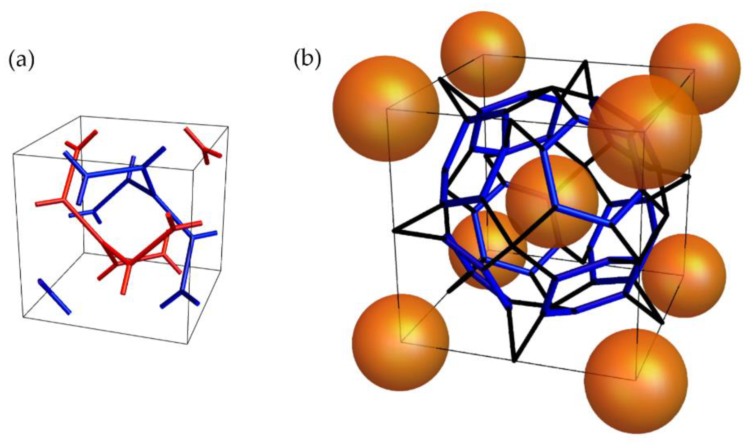
Unit cells of (a) a double gyroid cubic phase and (b) chiral cubic phase used to model the resonant X-ray response. The double gyroid cubic phase consists of two entangled systems of channels (red and blue). Three channels meet in a planar junction, and the direction normal to the junction rotates in the opposite direction in the two systems of channels. The all-hexagon-continuous grid of a chiral cubic phase consists of eight nonplanar hexagons (blue lines) in which the sides are of the same length as in the double gyroid phase, and hexagons consisting of two sides of the blue hexagons connected to the centers of edges and centers of faces of the cube (black lines). There are micelles in the center and edges of the unit cell. The unit cell side in the phase is always approximately longer than in the double gyroid phase.
Figure 1.
Unit cells of (a) a double gyroid cubic phase and (b) chiral cubic phase used to model the resonant X-ray response. The double gyroid cubic phase consists of two entangled systems of channels (red and blue). Three channels meet in a planar junction, and the direction normal to the junction rotates in the opposite direction in the two systems of channels. The all-hexagon-continuous grid of a chiral cubic phase consists of eight nonplanar hexagons (blue lines) in which the sides are of the same length as in the double gyroid phase, and hexagons consisting of two sides of the blue hexagons connected to the centers of edges and centers of faces of the cube (black lines). There are micelles in the center and edges of the unit cell. The unit cell side in the phase is always approximately longer than in the double gyroid phase.

Figure 2.
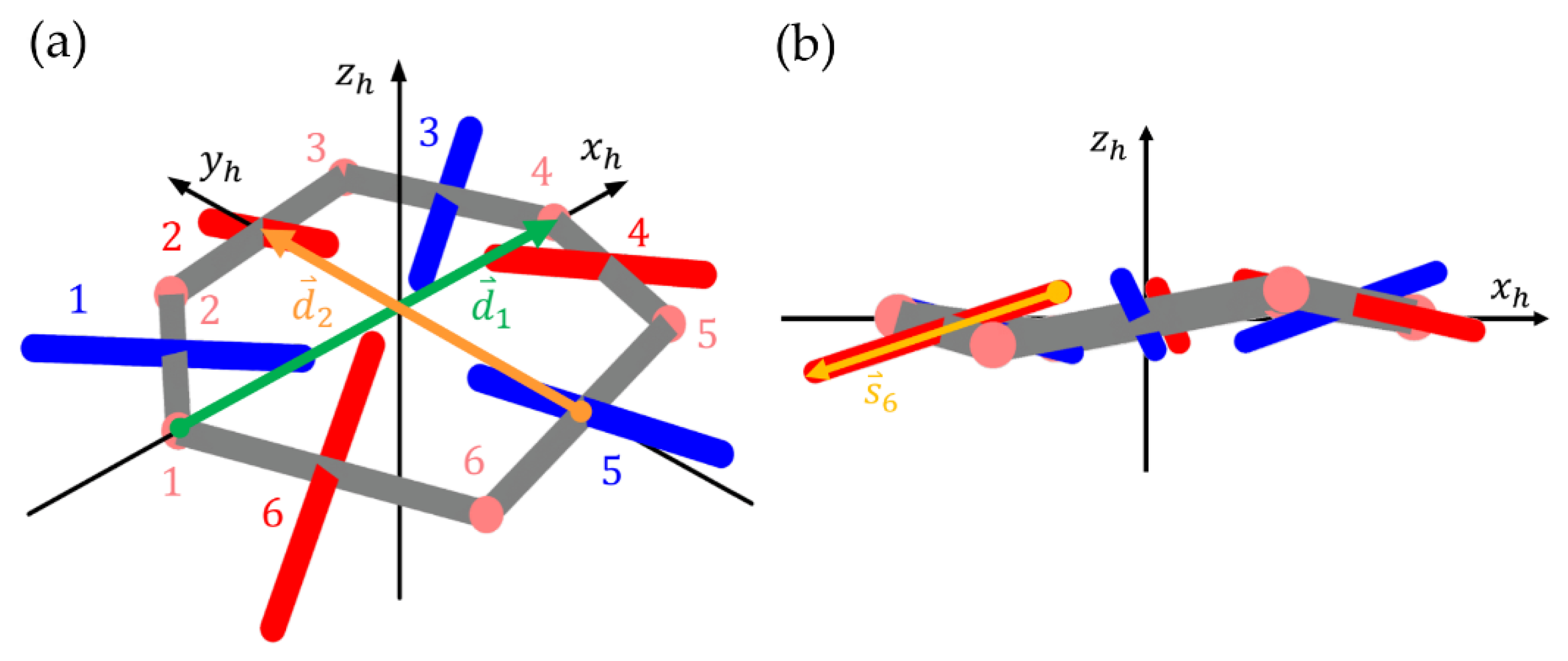
(a) A nonplanar hexagon in the coordinate system ( and ) centered on the hexagon. (b) A side view of the hexagon. Vector connects the opposite vertices of the hexagon that lie on the axis, and vector , which is perpendicular to , connects the opposite midpoints of the hexagon edges and points along the axis. Anisotropic scatterers (blue and red lines) are positioned perpendicular to each side of a hexagon. Inside the hexagon, the polarization axis of the blue scatterers is tilted in the direction by an angle and along the direction for the red scatterers. Scatterers, vertices and polarization axes are numbered from 1 to 6; thus determines the polarization axis of the -th scatterer.
Figure 2.
(a) A nonplanar hexagon in the coordinate system ( and ) centered on the hexagon. (b) A side view of the hexagon. Vector connects the opposite vertices of the hexagon that lie on the axis, and vector , which is perpendicular to , connects the opposite midpoints of the hexagon edges and points along the axis. Anisotropic scatterers (blue and red lines) are positioned perpendicular to each side of a hexagon. Inside the hexagon, the polarization axis of the blue scatterers is tilted in the direction by an angle and along the direction for the red scatterers. Scatterers, vertices and polarization axes are numbered from 1 to 6; thus determines the polarization axis of the -th scatterer.

Figure 3.
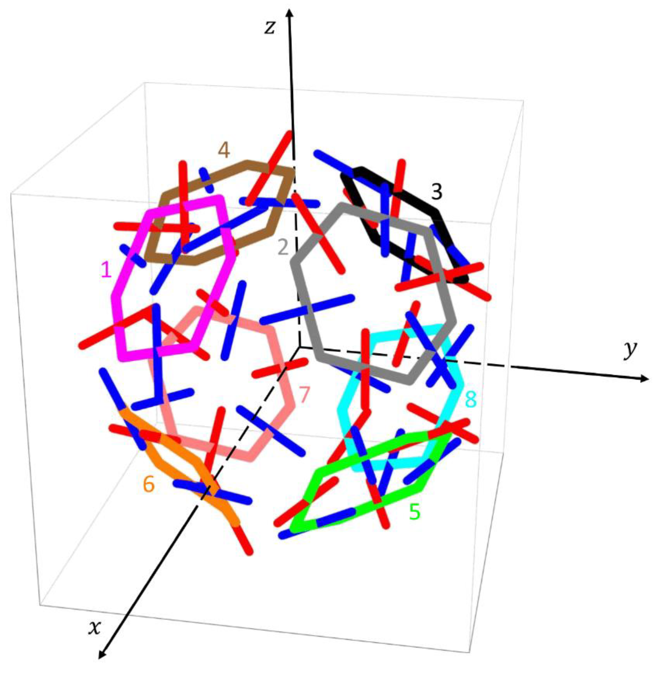
Hexagons in the unit cell of the chiral cubic phase in the laboratory system. Red and blue lines represent different inclinations of anisotropic scatterers with respect to the hexagon sides. All hexagons are identical (see Figure 2); they differ only by location and orientation inside the unit cell.
Figure 3.
Hexagons in the unit cell of the chiral cubic phase in the laboratory system. Red and blue lines represent different inclinations of anisotropic scatterers with respect to the hexagon sides. All hexagons are identical (see Figure 2); they differ only by location and orientation inside the unit cell.

Figure 4.
Scattering geometry for the peak with Miller indices () in the laboratory system. (a) is the scattering vector, and are the wave vectors of the incident and scattered wave, respectively; and are in-plane components of polarization of the incident and scattered wave, respectively, and and are perpendicular components. is the angle between the scattering vector and the axis and is the scattering angle. The angles between the wave vectors of the incident and scattered wave and the plane are and , respectively. (b) Projection of the scattering vector on the plane ( ) forms an angle with the axis.

Figure 5.
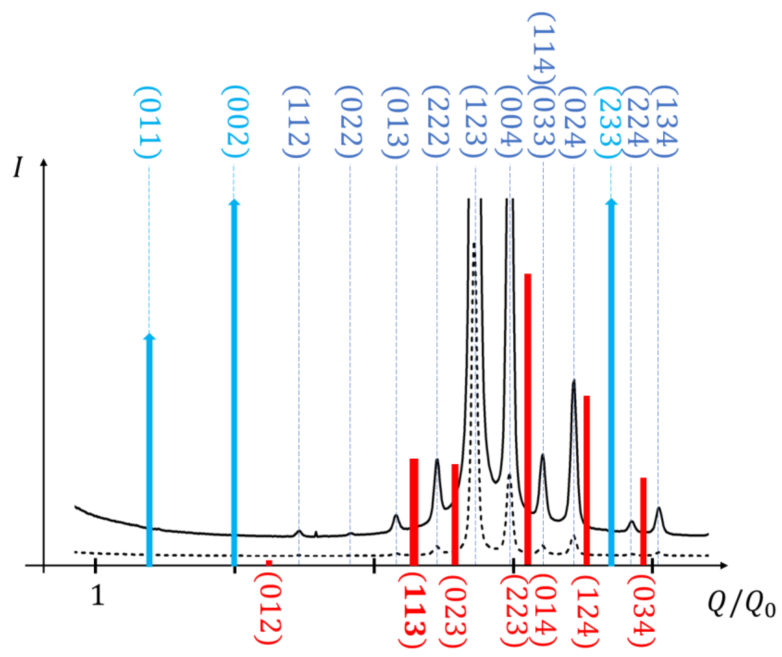
Intensities (in arbitrary units) of the diffracted peaks, measured by the nonresonant X-ray scattering (black curve) [11] and the predicted resonant (red lines) and resonantly enhanced peaks (blue arrows) as a function of the normalized scattering vector magnitude (), defined by the Miller indices : . The measured and calculated intensities are not to scale. The intensities are calculated at the scatterers’ inclination .
Figure 5.
Intensities (in arbitrary units) of the diffracted peaks, measured by the nonresonant X-ray scattering (black curve) [11] and the predicted resonant (red lines) and resonantly enhanced peaks (blue arrows) as a function of the normalized scattering vector magnitude (), defined by the Miller indices : . The measured and calculated intensities are not to scale. The intensities are calculated at the scatterers’ inclination .


Table 1.
Position () of the -th vertex of the hexagon and direction of the polarization axis for the -th scatterer in the case of an achiral hexagon ( in Figure 2) in the coordinate system centered on the hexagon (see Figure 2). Coordinates of vertices are given in units of the unit cell length ( ).
| 1 | ||
| 2 | ||
| 3 | ||
| 4 | ||
| 5 | ||
| 6 |
Table 2.
Coordinates of the centers of hexagons within the unit cell with a side length , unit vectors and along the direction of vectors and (see Figure 2) given in the laboratory coordinate system (,,) (Figure 3).
| (Color on Figure 3) | |||
|---|---|---|---|
| 1 (magenta) | |||
| 2 (gray) | |||
| 3 (black) | |||
| 4 (brown) | |||
| 5 (green) | |||
| 6 (orange) | |||
| 7 (pink) | |||
| 8 (cyan) |
Table 3.
Miller indices () of the resonant (green) and resonantly enhanced (orange) peaks predicted by the model and the corresponding tensor form factor ( ) in units of the tensor element ( ), for two inclinations of the polarization axis of scatterers ( ). Only those resonantly enhanced peaks are included that are not observed in the nonresonant X-ray scattering.
| (011) | ||
Table 4.
Relative intensities of peaks with Miller indices () and multiplicity , calculated at (RSoXS) and (TReXS) for the scatterer’s inclinations () and (). Intensities are normalized with the intensity of the peak () at the scatterer’s inclination ().
Table 4.
Relative intensities of peaks with Miller indices () and multiplicity , calculated at (RSoXS) and (TReXS) for the scatterer’s inclinations () and (). Intensities are normalized with the intensity of the peak () at the scatterer’s inclination ().
| 12 | (011) | RSoXS | ||
| 6 | (002) | |||
| 24 | (012) | |||
| 24 | (012) | TReXS | ||
| 24 | (113) | |||
| 24 | (023) | |||
| 24 | (014) | |||
| 24 | (223) | |||
| 48 | (124) | |||
| 24 | (233) | |||
| 24 | (034) |
Publisher’s Note: MDPI stays neutral with regard to jurisdictional claims in published maps and institutional affiliations. |
© 2021 by the authors. Licensee MDPI, Basel, Switzerland. This article is an open access article distributed under the terms and conditions of the Creative Commons Attribution (CC BY) license (http://creativecommons.org/licenses/by/4.0/).
Share and Cite
MDPI and ACS Style
Grabovac, T.; Gorecka, E.; Pociecha, D.; Vaupotič, N. Modeling of the Resonant X-ray Response of a Chiral Cubic Phase. Crystals 2021, 11, 214. https://0-doi-org.brum.beds.ac.uk/10.3390/cryst11020214
AMA Style
Grabovac T, Gorecka E, Pociecha D, Vaupotič N. Modeling of the Resonant X-ray Response of a Chiral Cubic Phase. Crystals. 2021; 11(2):214. https://0-doi-org.brum.beds.ac.uk/10.3390/cryst11020214
Chicago/Turabian StyleGrabovac, Timon, Ewa Gorecka, Damian Pociecha, and Nataša Vaupotič. 2021. "Modeling of the Resonant X-ray Response of a Chiral Cubic Phase" Crystals 11, no. 2: 214. https://0-doi-org.brum.beds.ac.uk/10.3390/cryst11020214
Note that from the first issue of 2016, this journal uses article numbers instead of page numbers. See further details here.