
A Framework for the Magnetic Dipole Effect on the Thixotropic Nanofluid Flow Past a Continuous Curved Stretched Surface

 , ,
, ,  ,
, 
Abstract
:1. Introduction
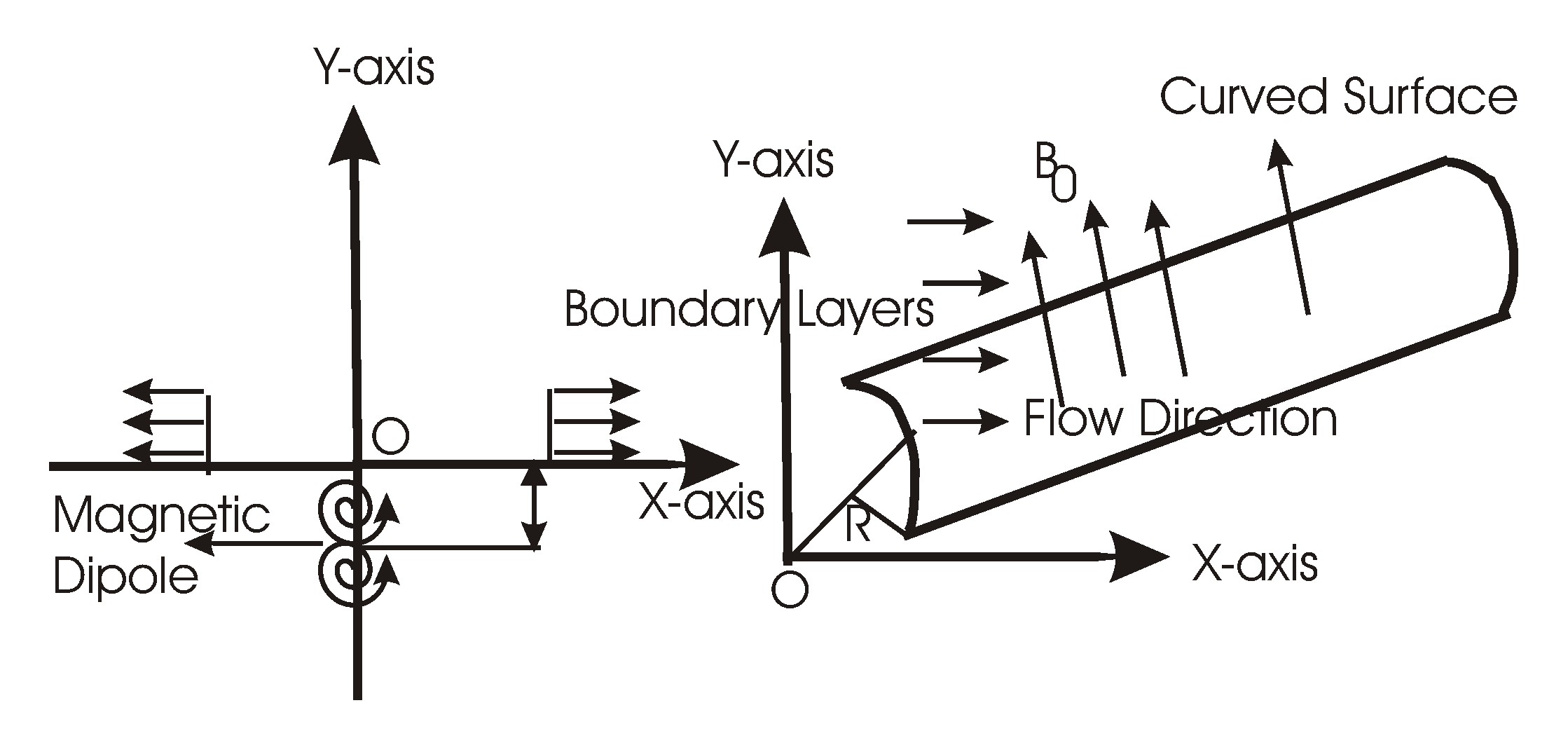
2. Methods
Magnetic Dipole
3. HAM Solution
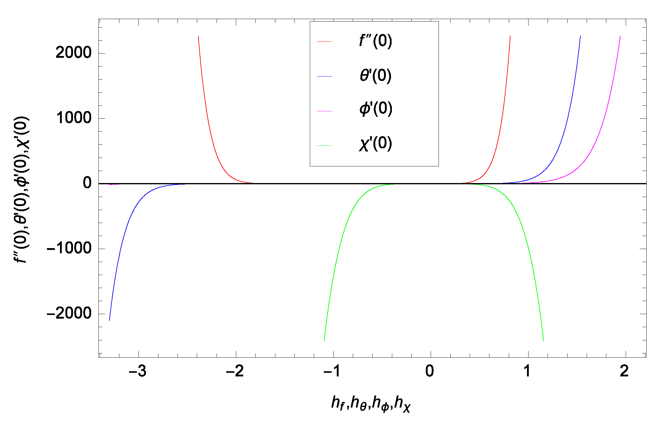
4. Convergence Analysis of the Homotopy Solution
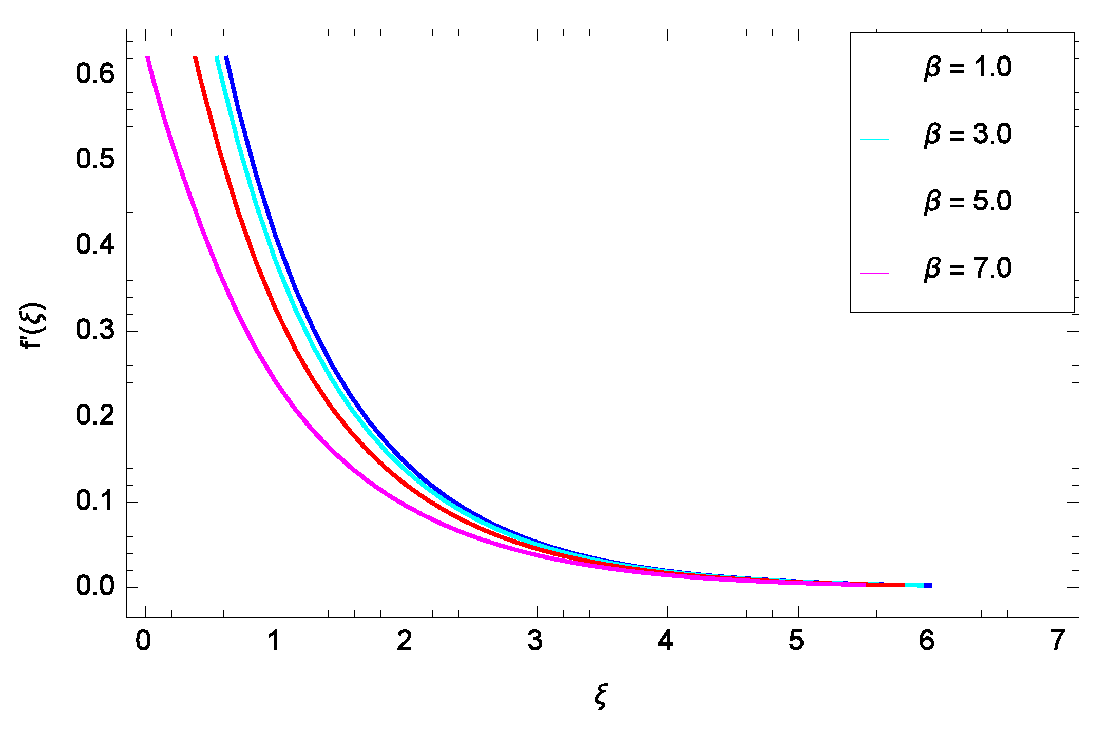
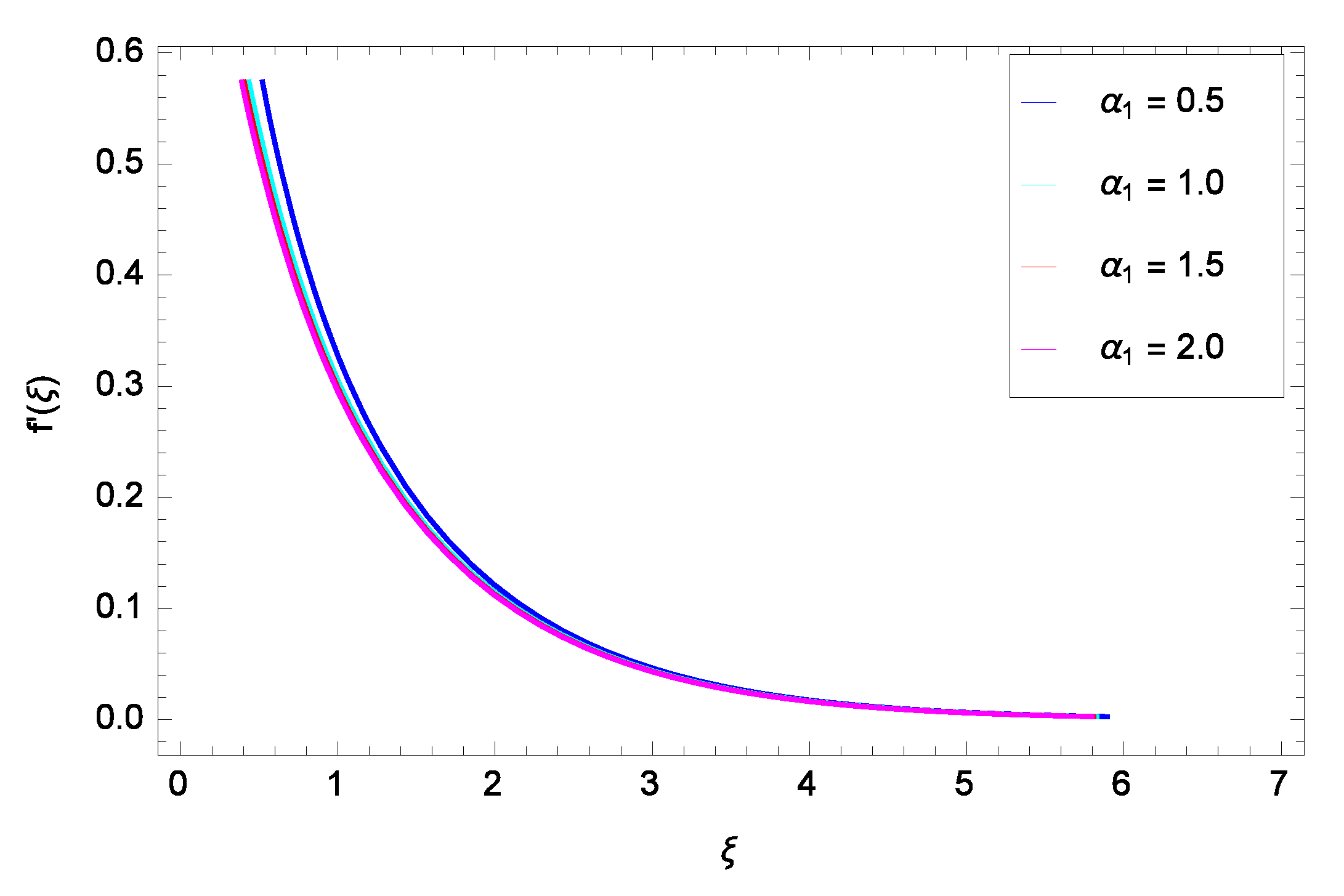
5. Discussion
6. Conclusions
- The velocity decreases with increasing values of ferromagnetic parameter and a curvature parameter , while it increases with increasing values of , and .
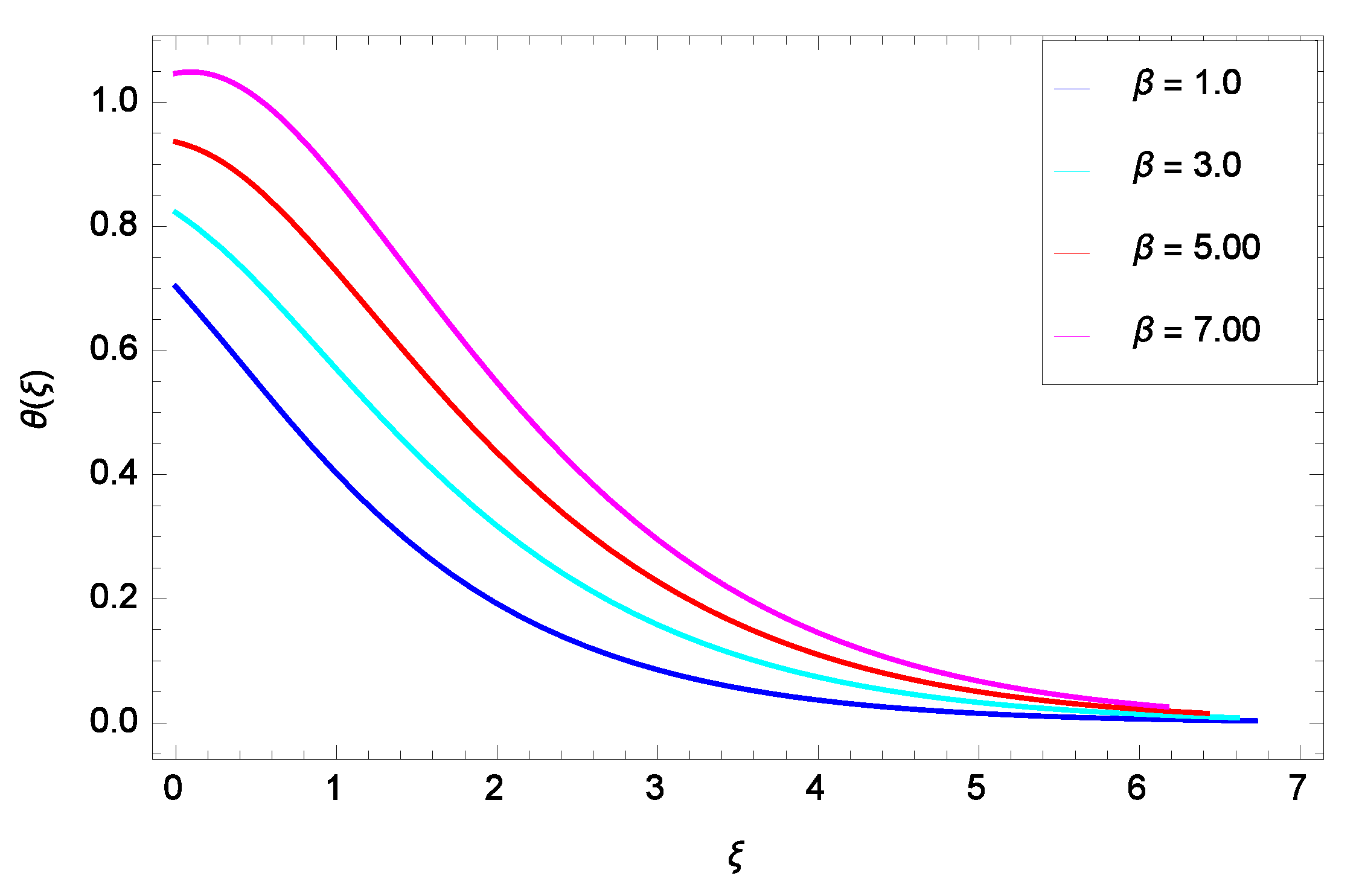
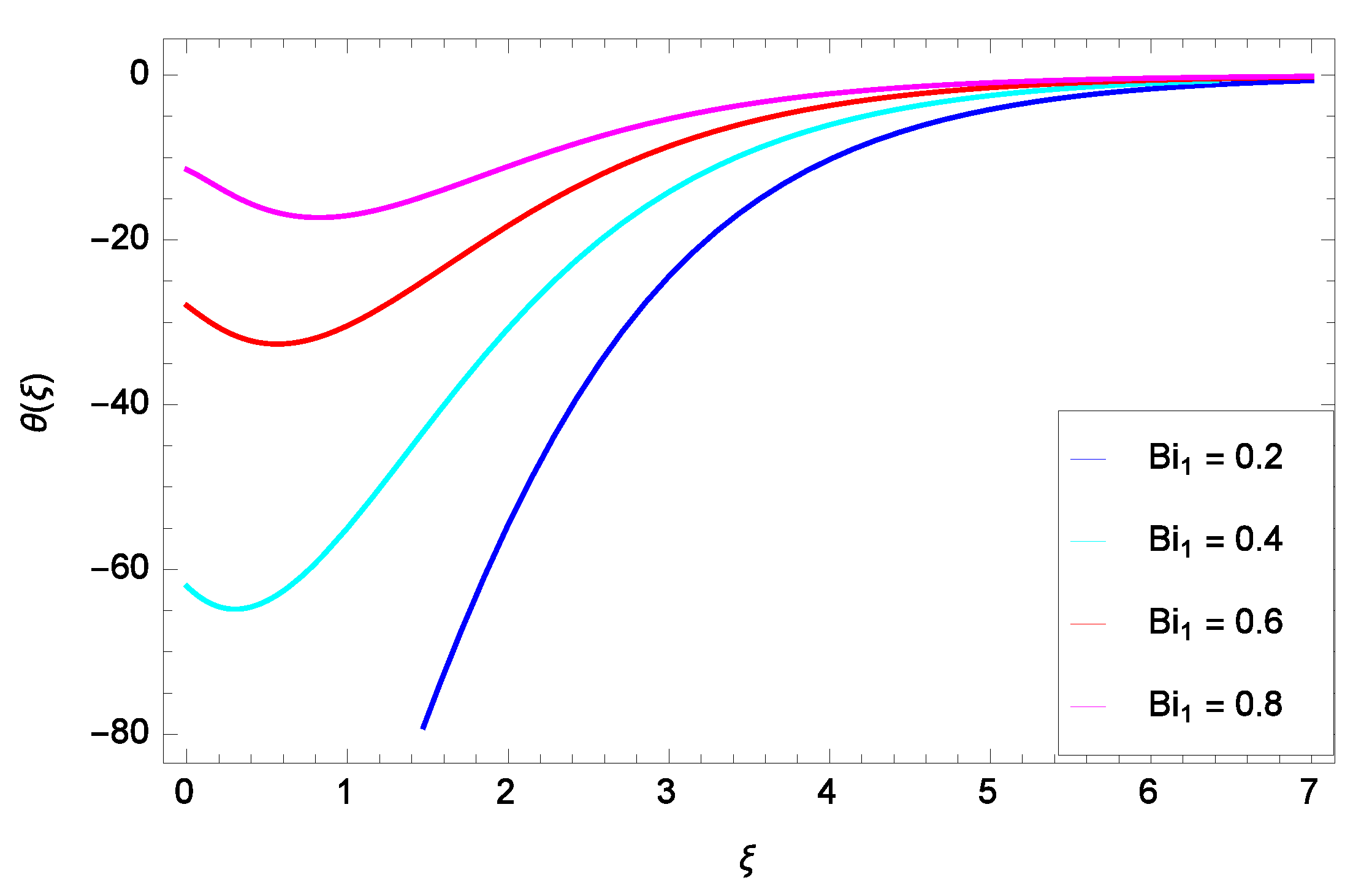
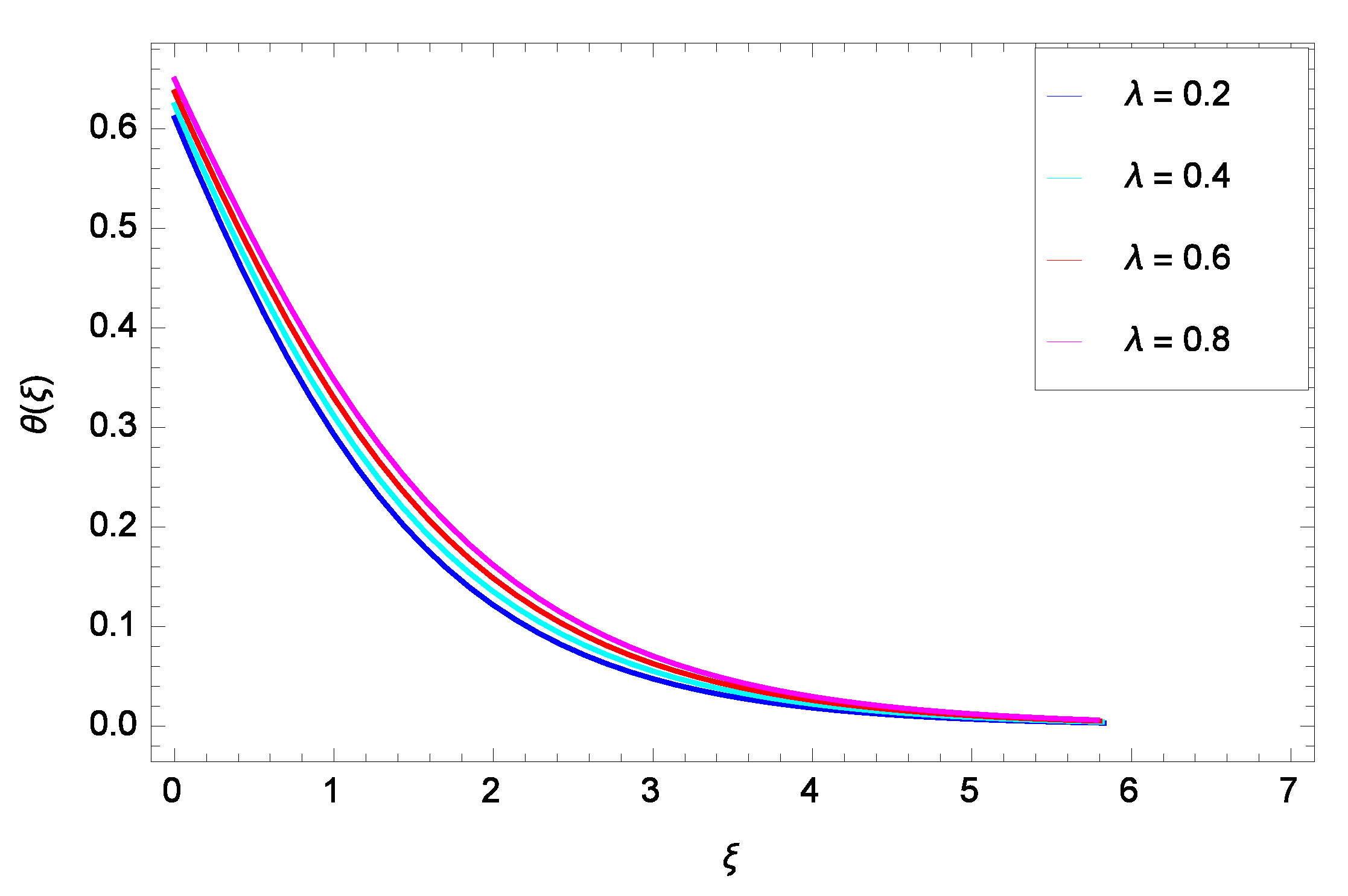
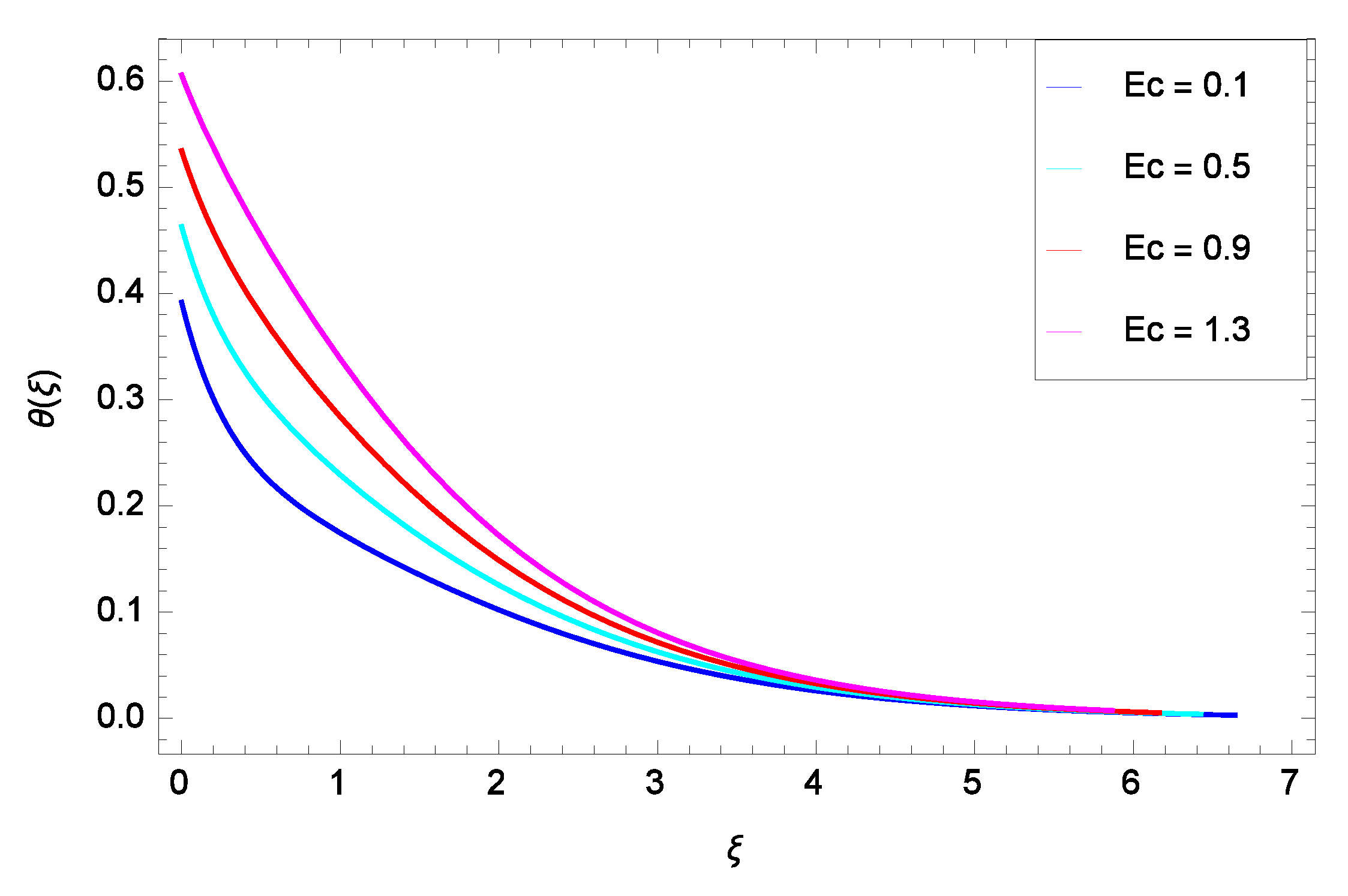
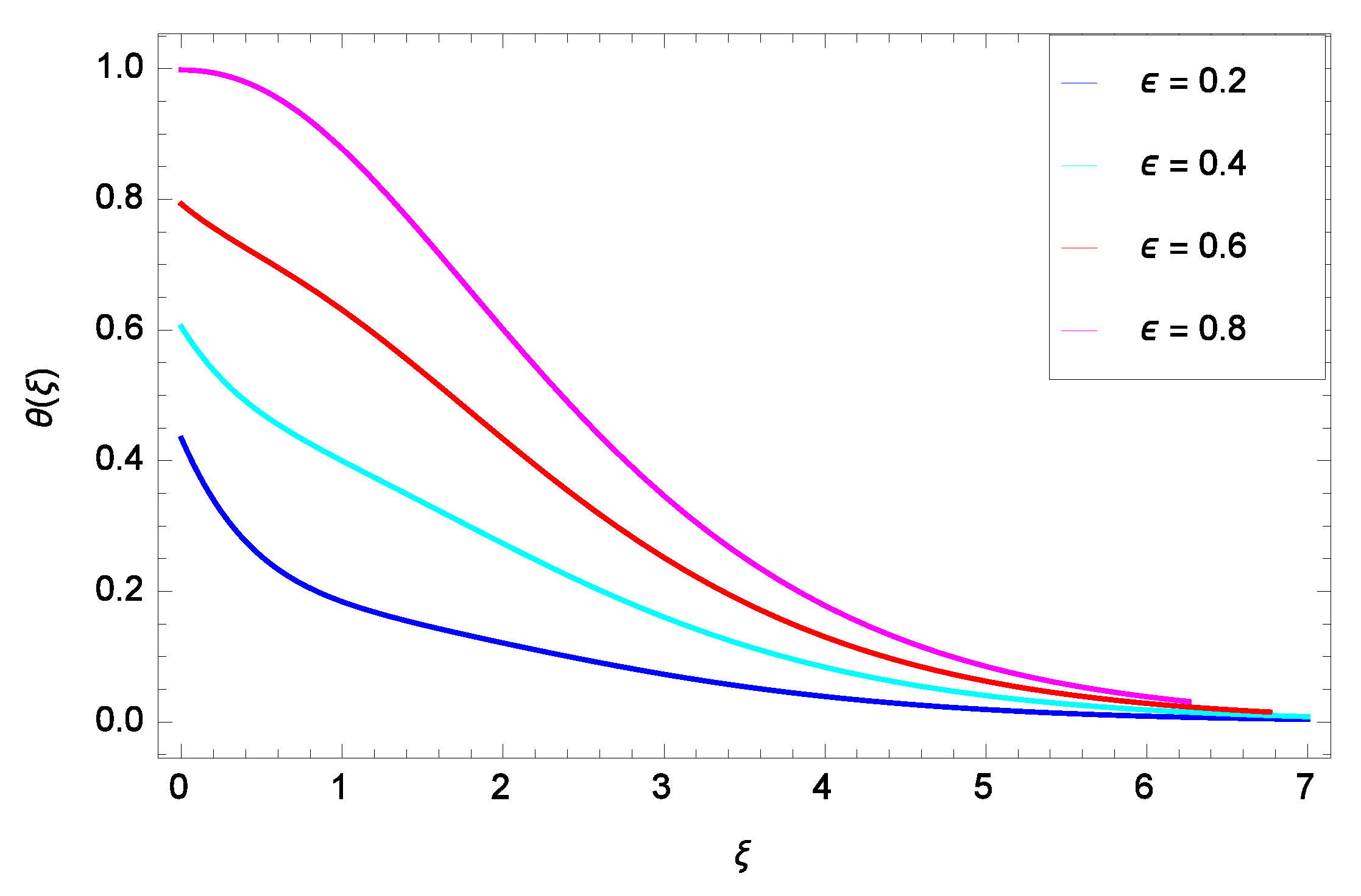
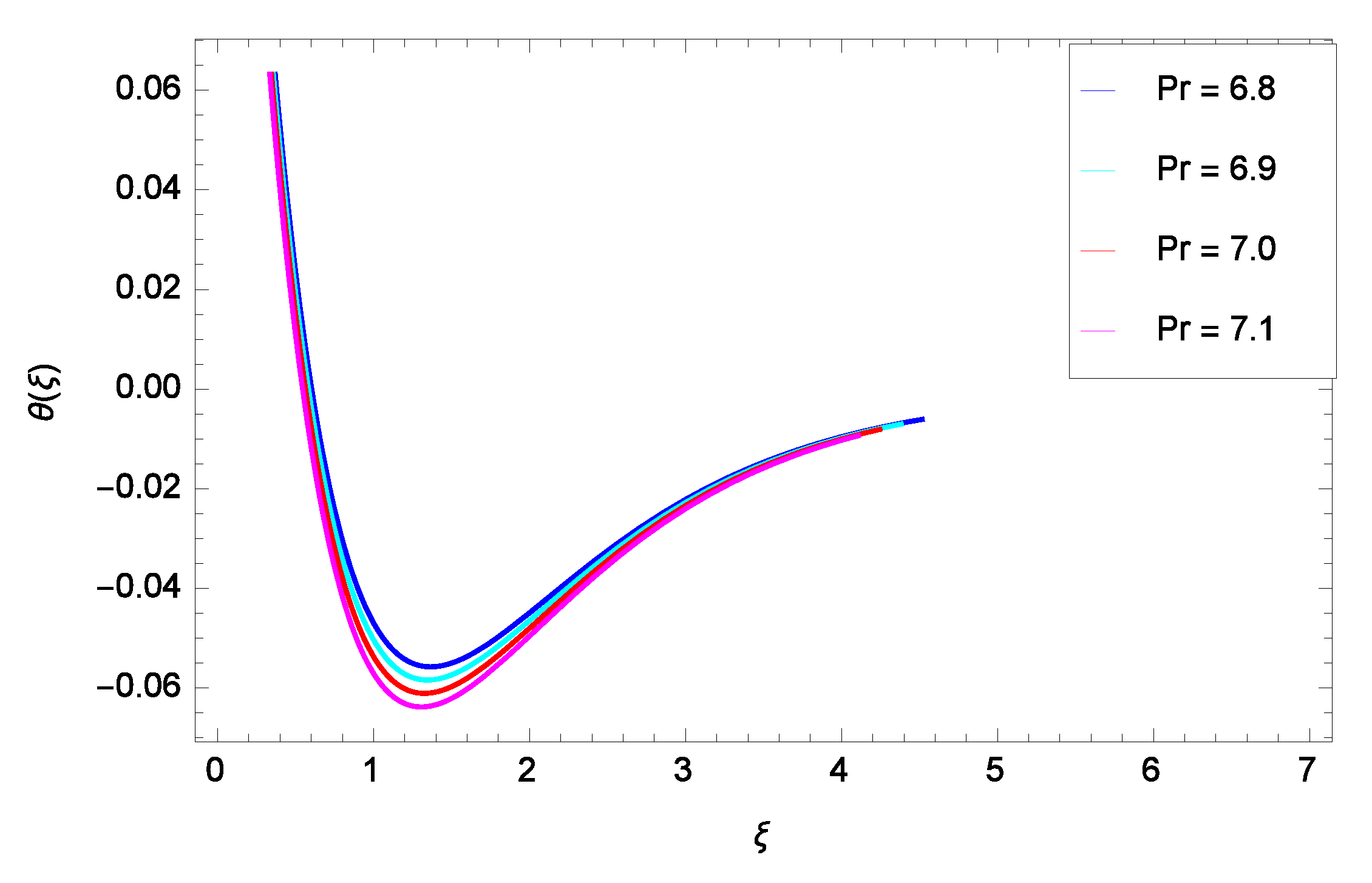
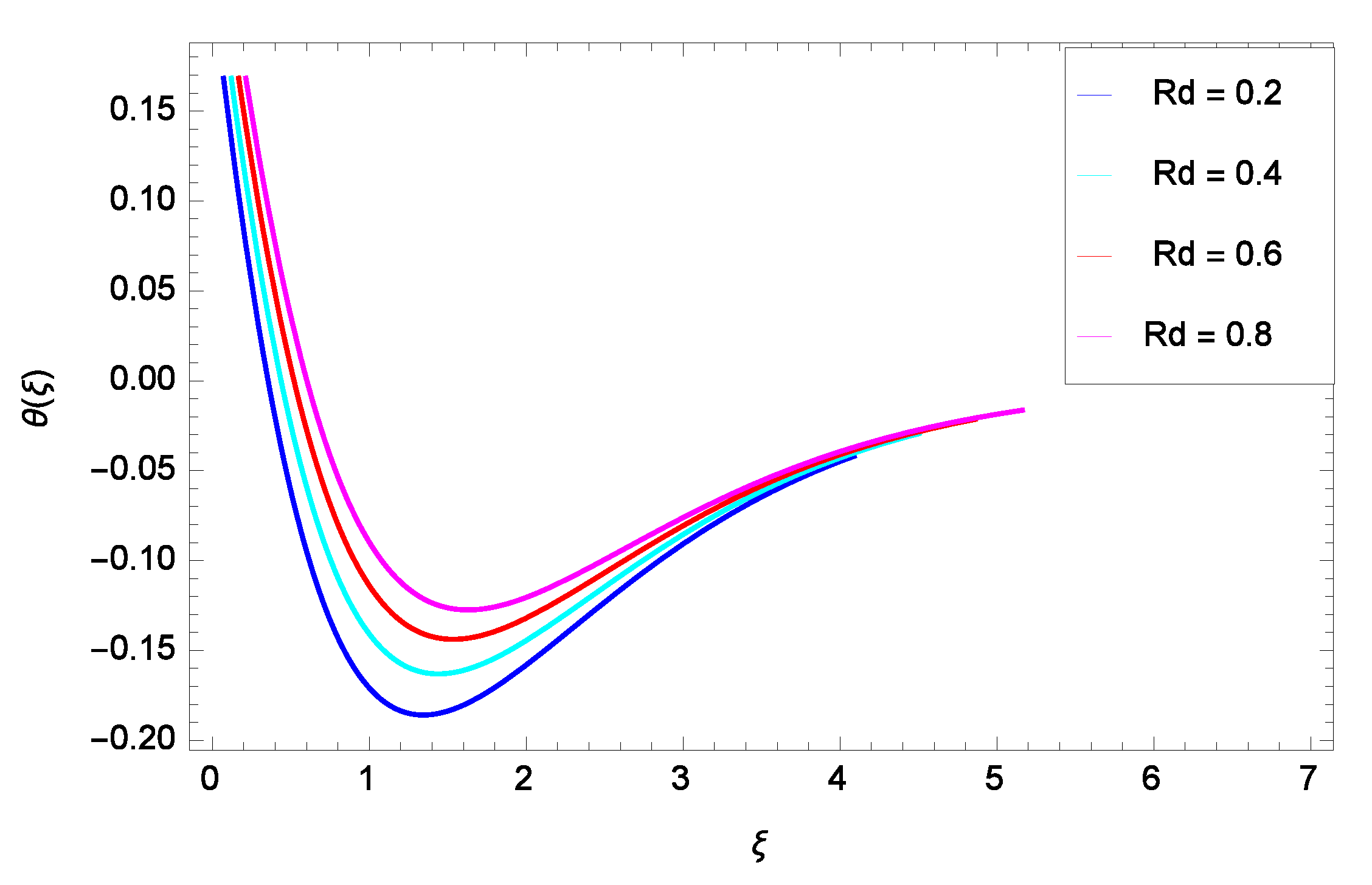
- The temperature increases with increasing values of , , and and decays with increasing values of .
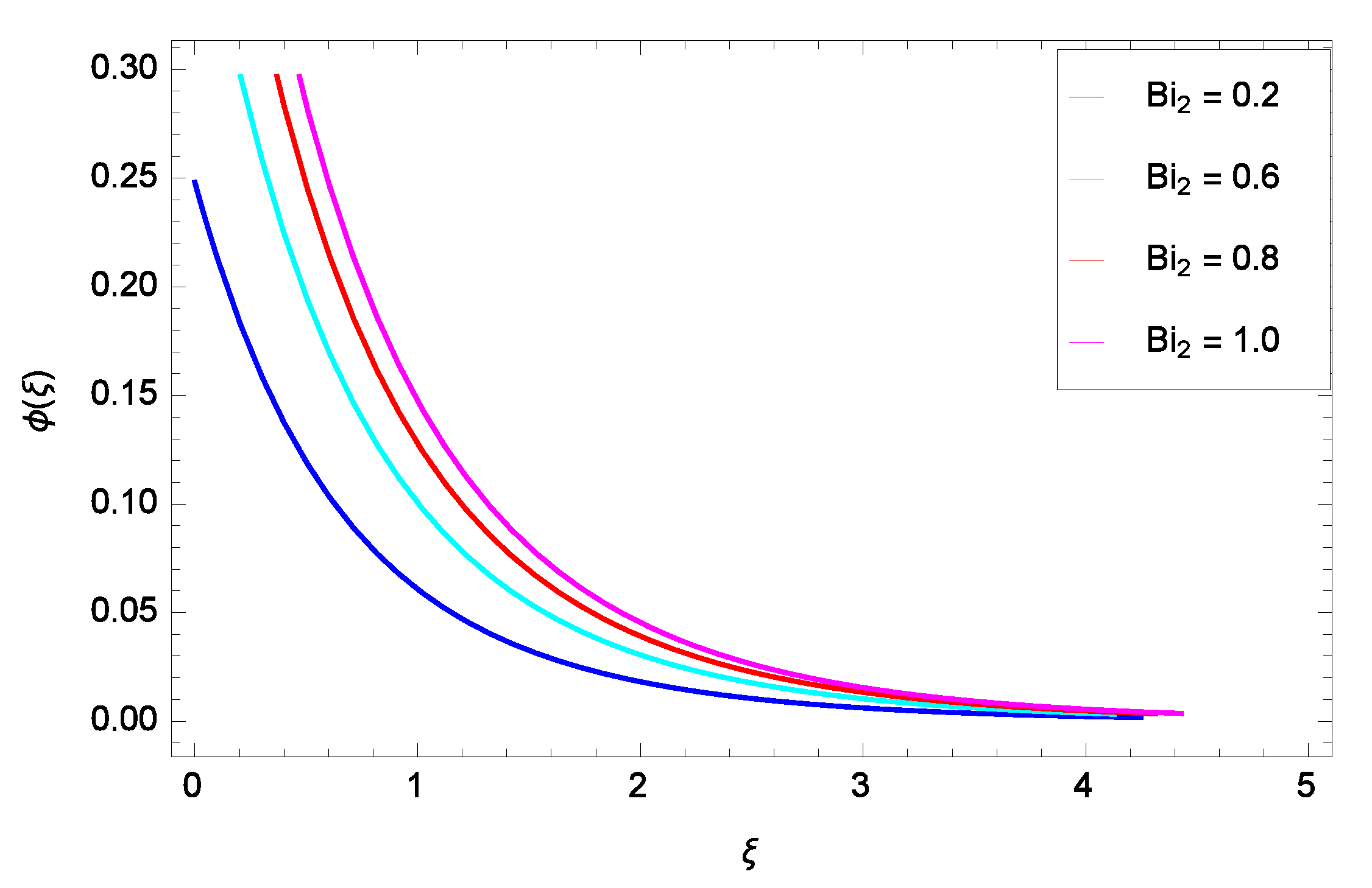
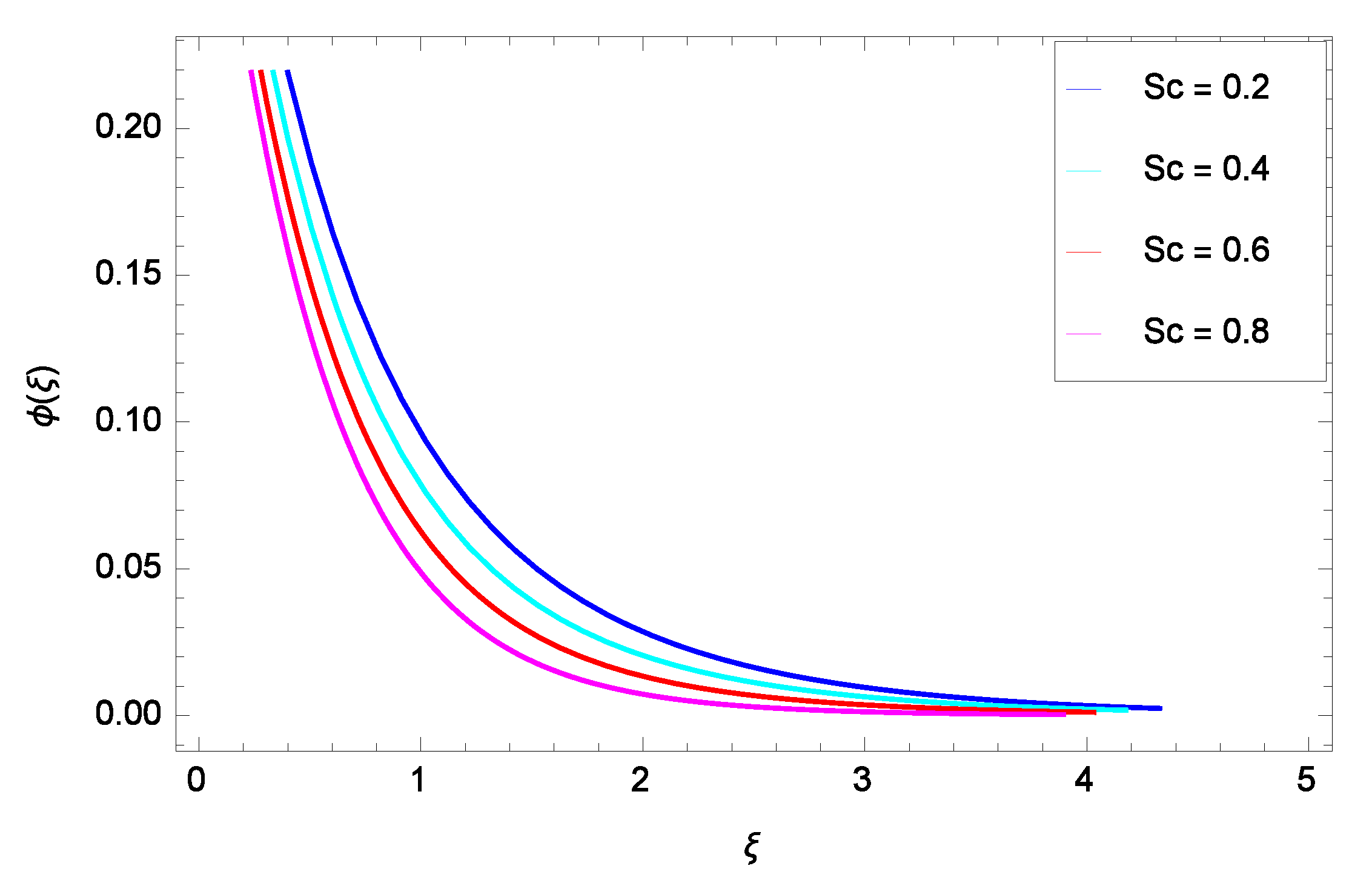
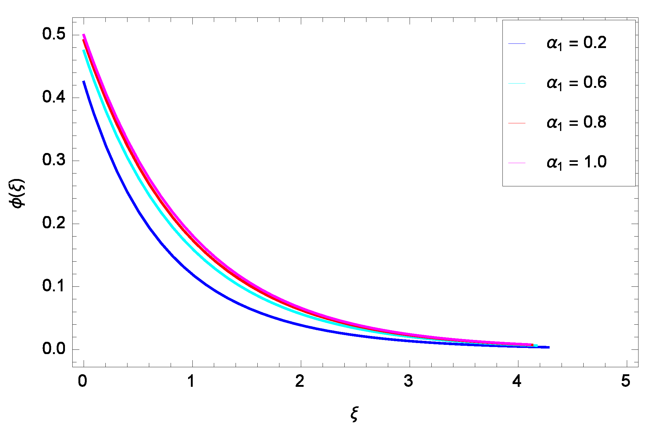
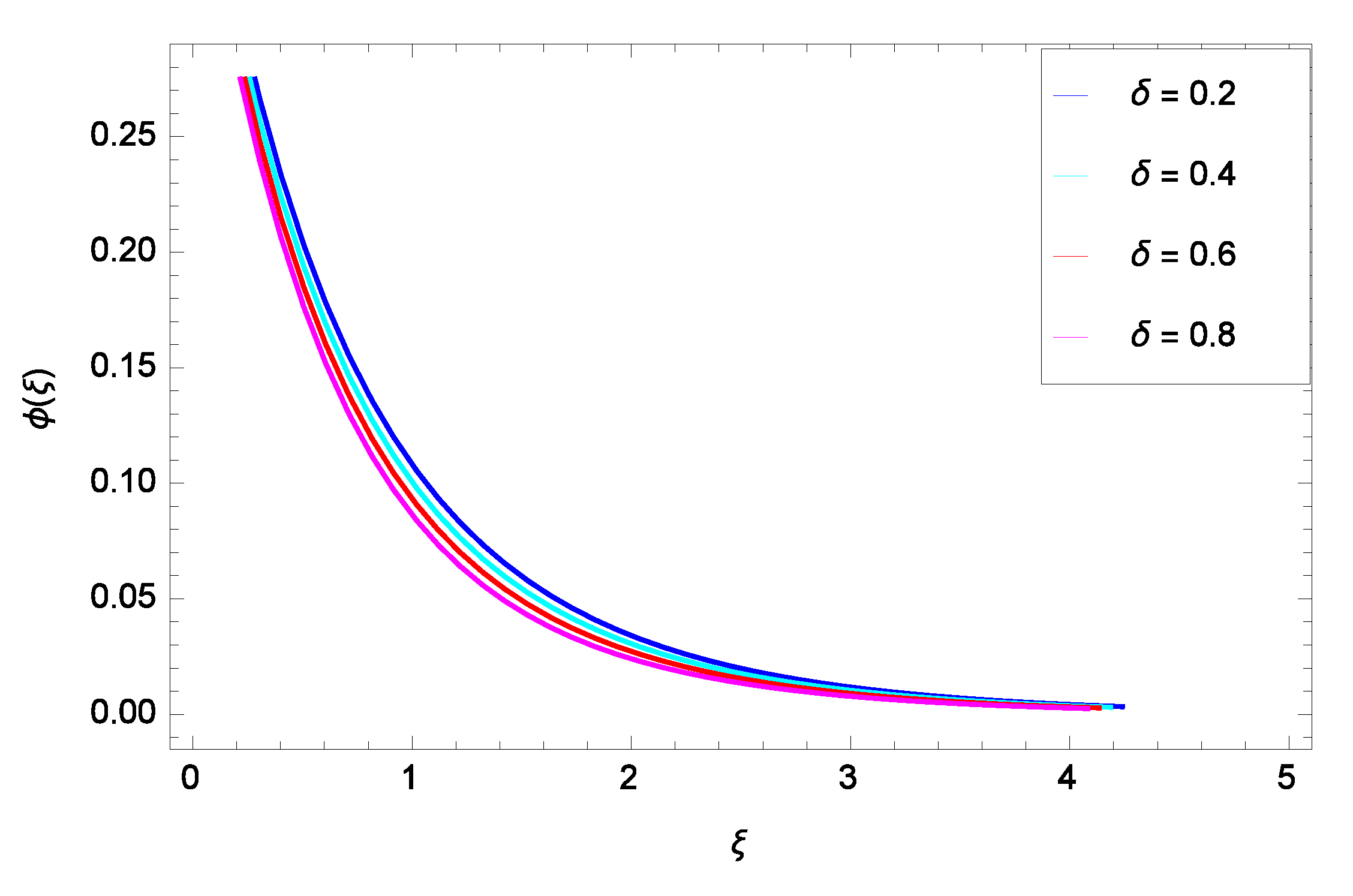
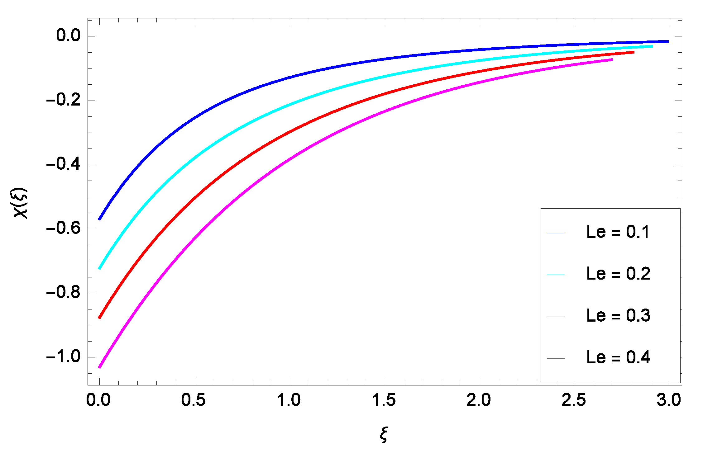
- The nanoparticles concentration decreases with increasing values of and , while it increases with increasing values of and .
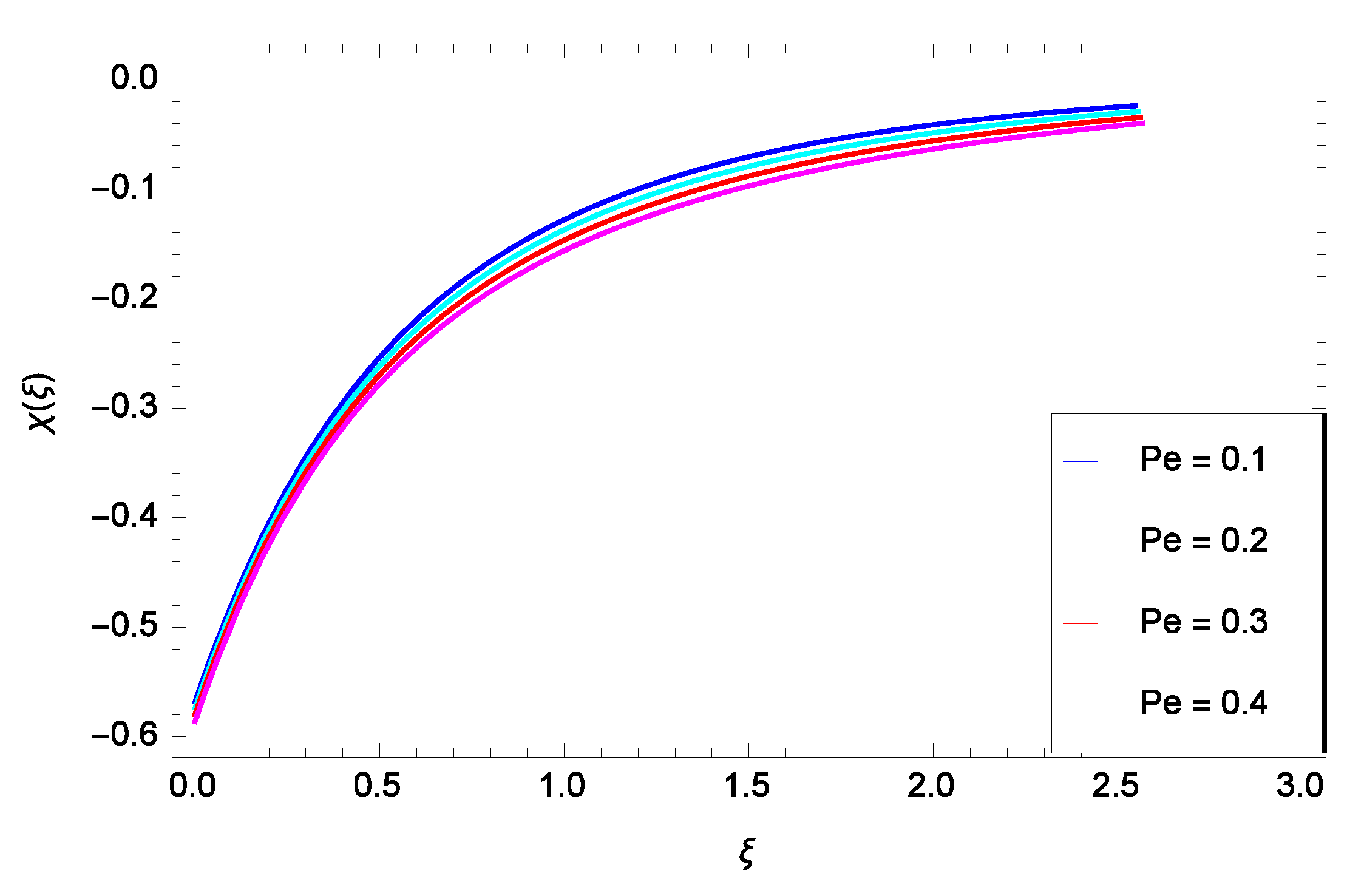
- The distribution of the microorganism is decreased with increasing values of and .
- The non-Newtonian parameters and have the same decreasing effects on the skin friction coefficient, while decreases and increases the heat transfer rate.
Author Contributions
Funding
Institutional Review Board Statement
Informed Consent Statement
Acknowledgments
Conflicts of Interest
References
- Ershkov, S.V. Non-stationary creeping flows for incompressible 3D Navier–Stokes equations. Eur. J. Mech. B/Fluids 2017, 61, 154–159. [Google Scholar] [CrossRef]
- Hsiao, K.L. Stagnation electrical MHD nanofluid mixed convection with slip boundary on a stretching sheet. Appl. Therm. Eng. 2016, 98, 850–861. [Google Scholar] [CrossRef]
- Hsiao, K.L. Micropolar nanofluid flow with MHD and viscous dissipation effects towards a stretching sheet with multimedia feature. Int. J. Heat Mass Transf. 2017, 112, 983–990. [Google Scholar] [CrossRef]
- Hsiao, K.L. Combined electrical MHD heat transfer thermal extrusion system using Maxwell fluid with radiative and viscous dissipation effects. Appl. Therm. Eng. 2017, 112, 1281–1288. [Google Scholar] [CrossRef]
- Hsiao, K.L. To promote radiation electrical MHD activation energy thermal extrusion manufacturing system efficiency by using Carreau-Nanofluid with parameters control method. Energy 2017, 130, 486–499. [Google Scholar] [CrossRef]
- de Deus, H.P.A.; Dupim, G.S. On behavior of the thixotropic fluids. Phys. Lett. A 2013, 377, 478–485. [Google Scholar] [CrossRef]
- Hayat, T.; Waqas, M.; Shehzad, S.A.; Alsaedi, A. A model of solar radiation and Joule heating in magnetohydrodynamic (MHD) convective flow of thixotropic nanofluid. J. Mol. Liq. 2016, 215, 704–710. [Google Scholar] [CrossRef]
- Hayat, T.; Waqas, M.; Khan, M.I.; Alsaedi, A. Analysis of thixotropic nanomaterial in a doubly stratified medium considering magnetic field effects. Int. J. Heat Mass Transf. 2016, 102, 1123–1129. [Google Scholar] [CrossRef]
- Zubair, M.; Waqas, M.; Hayat, T.; Ayub, M.; Alsaedi, A. Simulation of nonlinear convective thixotropic liquid with Cattaneo-Christov heat flux. Results Phys. 2018, 8, 1023–1027. [Google Scholar] [CrossRef]
- Khan, N.S.; Shah, Z.; Islam, S.; Khan, I.; Alkanhal, T.A.; Tlili, T. Entropy generation in MHD mixed convection non-Newtonian second-grade nanoliquid thin film flow through a porous medium with chemical reaction and stratification. Entropy 2019, 21, 139. [Google Scholar] [CrossRef] [Green Version]
- Khan, N.S.; Gul, T.; Islam, S.; Khan, W. Thermophoresis and thermal radiation with heat and mass transfer in a magnetohydrodynamic thin film second-grade fluid of variable properties past a stretching sheet. Eur. Phys. J. Plus 2017, 132, 11. [Google Scholar] [CrossRef]
- Palwasha, Z.; Khan, N.S.; Shah, Z.; Islam, S.; Bonyah, E. Study of two dimensional boundary layer thin film fluid flow with variable thermo-physical properties in three dimensions space. AIP Adv. 2018, 8, 105318. [Google Scholar] [CrossRef] [Green Version]
- Khan, N.S.; Gul, T.; Islam, S.; Khan, A.; Shah, Z. Brownian motion and thermophoresis effects on MHD mixed convective thin film second-grade nanofluid flow with Hall effect and heat transfer past a stretching sheet. J. Nanofluids 2017, 6, 812–829. [Google Scholar] [CrossRef]
- Khan, N.S.; Zuhra, S.; Shah, Z.; Bonyah, E.; Khan, W.; Islam, S. Slip flow of Eyring-Powell nanoliquid film containing graphene nanoparticles. AIP Adv. 2019, 8, 115302. [Google Scholar] [CrossRef]
- Khan, N.S.; Gul, T.; Kumam, P.; Shah, Z.; Islam, S.; Khan, W.; Zuhra, S.; Sohail, A. Influence of inclined magnetic field on Carreau nanoliquid thin film flow and heat transfer with graphene nanoparticles. Energies 2019, 12, 1459. [Google Scholar] [CrossRef] [Green Version]
- Khan, N.S. Study of two dimensional boundary layer flow of a thin film second grade fluid with variable thermo-physical properties in three dimensions space. Filomat 2019, 33, 5387–5405. [Google Scholar] [CrossRef] [Green Version]
- Khan, N.S.; Zuhra, S. Boundary layer unsteady flow and heat transfer in a second grade thin film nanoliquid embedded with graphene nanoparticles past a stretching sheet. Adv. Mech. Eng. 2019, 11, 1–11. [Google Scholar] [CrossRef] [Green Version]
- Khan, N.S.; Gul, T.; Islam, S.; Khan, W.; Khan, I.; Ali, L. Thin film flow of a second-grade fluid in a porous medium past a stretching sheet with heat transfer. Alex. Eng. J. 2017, 57, 1019–1031. [Google Scholar] [CrossRef]
- Zahra, A.; Mahanthesh, B.; Basir, M.F.M.; Imtiaz, M.; Mackolil, J.; Khan, N.S.; Nabwey, H.A.; Tlili, I. Mixed radiated magneto Casson fluid flow with Arrhenius activation energy and Newtonian heating effects: Flow and sensitivity analysis. Alex. Eng. J. 2020, 57, 1019–1031. [Google Scholar]
- Liaqat, A.; Asifa, T.; Ali, R.; Islam, S.; Gul, T.; Kumam, P.; Mukhtar, S.; Khan, N.S.; Thounthong, P. A new analytical approach for the research of thin-film flow of magneto hydrodynamic fluid in the presence of thermal conductivity and variable viscosity. ZAMM J. Appl. Math. Mech. Z. Angewwandte Math. Mech. 2020, 1–13. [Google Scholar] [CrossRef]
- Khan, N.S.; Zuhra, S.; Shah, Z.; Bonyah, E.; Khan, W.; Islam, S.; Khan, A. Hall current and thermophoresis effects on magnetohydrodynamic mixed convective heat and mass transfer thin film flow. J. Phys. Commun. 2019, 3, 035009. [Google Scholar] [CrossRef]
- Nield, D.A.; Bejan, A. Convection in Porous Media; Springer: New York, NY, USA, 2006; p. 3. [Google Scholar]
- Forchheimer, P. Wasserbewegung durch boden. Z. Ver. Dtsch. Ing. 1901, 45, 1782–1788. [Google Scholar]
- Morris, M. The Flow of Homogeneous Fluids through Porous Media; J.W. Edwards Inc.: Ann Arbor, MI, USA, 1946; p. 191. [Google Scholar]
- Kishan, N.; Maripala, S. Thermophoresis and viscous dissipation effects on Darcy–Forchheimer MHD mixed convection in a fluid saturated porous media. Adv. Appl. Sci. Res. 2012, 3, 60–74. [Google Scholar]
- Rauf, A.; Abbas, Z.; Shehzad, S.A.; Mushtaq, T. Thermally radiative viscous fluid flow over curved moving surface in Darcy–Forchheimer porous space. Commun. Theor. Phys. 2019, 71, 259. [Google Scholar] [CrossRef]
- Jagadha, S.; Amrutha, P. MHD boundary layer flow of Darcy-Forchheimer mixed convection in a nanofluid saturated porous media with viscous dissipation. Int. J. Appl. Appl. Math. 2019, 4, 117–134. [Google Scholar]
- Andersson, H.I.; Valnes, O.A. Flow of a heated ferrofluid over a stretching sheet in the presence of a magnetic dipole. Acta Mech. 1998, 128, 39–47. [Google Scholar] [CrossRef]
- Hayat, T.; Ahmad, S.; Khan, M.I.; Alsaedi, A. Exploring magnetic dipole contribution on radiative flow of ferromagnetic Williamson fluid. Results Phys. 2018, 8, 545–551. [Google Scholar] [CrossRef]
- Titus, L.R.; Abraham, A. Heat transfer in ferrofluid flow over a stretching sheet with radiation. Int. J. Eng. Res. Technol. 2014, 3, 2198–2203. [Google Scholar]
- Kefayati, G.H. Natural convection of ferrofluid in a linearly heated cavity utilizing LBM. J. Mol. Liq. 2014, 191, 1–9. [Google Scholar] [CrossRef]
- Afkhami, S.; Renardy, Y. Ferrofluids and magnetically guided superparamagnetic particles in flows: A review of simulations and modeling. J. Eng. Math. 2017, 107, 231–251. [Google Scholar] [CrossRef] [Green Version]
- Mabood, F.; Khan, W.A.; Ismail, A.M. MHD stagnation point flow and heat transfer impinging on stretching sheet with chemical reaction and transpiration. Chem. Eng. J. 2015, 273, 430–437. [Google Scholar] [CrossRef]
- Narayana, P.S.; Babu, D.H. Numerical study of MHD heat and mass transfer of a Jeffrey fluid over a stretching sheet with chemical reaction and thermal radiation. J. Taiwan Inst. Chem. Eng. 2016, 59, 18–25. [Google Scholar] [CrossRef]
- Hayat, T.; Zahir, H.; Tanveer, A.; Alsaedi, A. Influences of Hall current and chemical reaction in mixed convective peristaltic flow of Prandtl fluid. J. Magn. Magn. Mater. 2016, 407, 321–327. [Google Scholar] [CrossRef]
- Hayat, T.; Rashid, M.; Imtiaz, M.; Alsaedi, A. MHD convective flow due to a curved surface with thermal radiation and chemical reaction. J. Mol. Liq. 2017, 225, 482–489. [Google Scholar] [CrossRef]
- Khan, N.S.; Gul, T.; Islam, S.; Khan, I.; Alqahtani, A.M.; Alshomrani, A.S. Magnetohydrodynamic nanoliquid thin film sprayed on a stretching cylinder with heat transfer. J. Appl. Sci. 2017, 7, 271. [Google Scholar] [CrossRef]
- Khan, N.S.; Kumam, P.; Thounthong, P. Renewable energy technology for the sustainable development of thermal system with entropy measures. Int. J. Heat Mass Transf. 2019, 145, 118713. [Google Scholar] [CrossRef]
- Khan, N.S.; Kumam, P.; Thounthong, P. Second law analysis with effects of Arrhenius activation energy and binary chemical reaction on nanofluid flow. Sci. Rep. 2020, 10, 1226. [Google Scholar] [CrossRef] [PubMed] [Green Version]
- Khan, N.S.; Shah, Q.; Bhaumik, A.; Kumam, P.; Thounthong, P.; Amiri, I. Entropy generation in bioconvection nanofluid flow between two stretchable rotating disks. Sci. Rep. 2020, 10, 4448. [Google Scholar] [CrossRef] [PubMed]
- Khan, N.S.; Shah, Q.; Sohail, A. Dynamics with Cattaneo-Christov heat and mass flux theory of bioconvection Oldroyd-B nanofluid. Adv. Mech. Eng. 2020, 12, 1–20. [Google Scholar] [CrossRef]
- Khan, N.S.; Shah, Q.; Sohail, A.; Kumam, P.; Thounthong, P.; Bhaumik, A.; Ullah, Z. Lorentz forces effects on the interactions of nanoparticles in emerging mechanisms with innovative approach. Symmetry 2020, 5, 1700. [Google Scholar] [CrossRef]
- Liaqat, A.; Khan, N.S.; Ali, R.; Islam, S.; Kumam, P.; Thounthong, P. Novel insights through the computational techniques in unsteady MHD second grade fluid dynamics with oscillatory boundary conditions. Heat Transf. 2020, 50, 2502–2524. [Google Scholar] [CrossRef]
- Chamkha, A.J.; Rashad, A.M.; Kameswaran, P.K.; Abdou, M.M. Radiation effects on natural bioconvection flow of a nanofluid containing gyrotactic microorganisms past a vertical plate with streamwise temperature variation. J. Nanofluids 2017, 6, 587–595. [Google Scholar] [CrossRef]
- Raju, C.S.; Seep, N. Dual solutions for unsteady heat and mass transfer in bio-convection flow towards a rotating cone/plate in a rotating fluid. Int. J. Eng. Res. Afr. 2016, 20, 161–176. [Google Scholar] [CrossRef]
- Hady, F.M.; Mahdy, A.; Mohamed, R.A.; Zaid, O.A.A. Effects of viscous dissipation on unsteady MHD thermo bioconvection boundary layer flow of a nanofluid containing gyrotactic microorganisms along a stretching sheet. World J. Mech. 2016, 6, 505–526. [Google Scholar] [CrossRef] [Green Version]
- Khan, N.S. Bioconvection in second grade nanofluid flow containing nanoparticles and gyrotactic microorganisms. Braz. J. Phys. 2018, 48, 227–241. [Google Scholar] [CrossRef]
- Ferdows, M.; Zaimi, K.; Rashad, A.M.; Nabwey, H.A. MHD bioconvection flow and heat transfer of nanofluid through an exponentially stretchable sheet. Symmetry 2020, 12, 692. [Google Scholar] [CrossRef]
- Khan, S.U.; Al-Khaled, K.; Bhatti, M.M. Bioconvection analysis for flow of Oldroyd-B nanofluid configured by a convectively heated surface with partial slip effects. Surf. Interfaces 2021, 23, 100982. [Google Scholar] [CrossRef]
- Majeed, A.; Zeeshan, A.; Amin, N.; Ijaz, N.; Saeed, T. Thermal analysis of radiative bioconvection magnetohydrodynamic flow comprising gyrotactic microorganism with activation energy. J. Therm. Anal. Calorim. 2021, 143, 2545–2556. [Google Scholar] [CrossRef]
- Zuhra, S.; Khan, N.S.; Alam, A.; Islam, S.; Khan, A. Buoyancy effects on nanoliquids film flow through a porous medium with gyrotactic microorganisms and cubic autocatalysis chemical reaction. Adv. Mech. Eng. 2020, 12, 1–17. [Google Scholar] [CrossRef] [Green Version]
- Palwasha, Z.; Islam, S.; Khan, N.S.; Ayaz, H. Non-Newtonian nanoliquids thin film flow through a porous medium with magnetotactic microorganisms. Appl. Nanosci. 2018, 8, 1523–1544. [Google Scholar] [CrossRef]
- Khan, N.S. Mixed convection in MHD second grade nanofluid flow through a porous medium containing nanoparticles and gyrotactic microorganisms with chemical reaction. Filomat 2019, 33, 4627–4653. [Google Scholar] [CrossRef] [Green Version]
- Zuhra, S.; Khan, N.S.; Shah, Z.; Islam, Z.; Bonyah, E. Simulation of bioconvection in the suspension of second grade nanofluid containing nanoparticles and gyrotactic microorganisms. AIP Adv. 2018, 8, 105210. [Google Scholar] [CrossRef] [Green Version]
- Khan, N.S.; Shah, Z.; Shutaywi, M.; Kumam, P.; Thounthong, P. A comprehensive study to the assessment of Arrhenius activation energy and binary chemical reaction in swirling flow. Sci. Rep. 2020, 10, 7868. [Google Scholar] [CrossRef] [PubMed]
- Khan, N.S.; Gul, T.; Khan, M.A.; Bonyah, E.; Islam, S. Mixed convection in gravity-driven thin film non-Newtonian nanofluids flow with gyrotactic microorganisms. Results Phys. 2017, 7, 4033–4049. [Google Scholar] [CrossRef]
- Liao, S.J. An explicit, totally analytic approximate solution for Blasius’ viscous flow problems. Int. J. Non-Linear Mech. 1999, 34, 759–778. [Google Scholar] [CrossRef]
- Liao, S. Beyond Perturbation: Introduction to the Homotopy Analysis Method; CRC Press: Boca Raton, FL, USA, 2003. [Google Scholar]
- Liao, S.J. Homotopy Analysis Method in Nonlinear Differential Equations; Higher Education Press: Beijing, China; Springer: Berlin/Heidelberg, Germany, 2012. [Google Scholar]
- Shah, Z.; Islam, S.; Gul, T.; Bonyah, E.; Khan, M.A. The electrical MHD and hall current impact on micropolar nanofluid flow between rotating parallel plates. Results Phys. 2018, 9, 1201–1214. [Google Scholar] [CrossRef]
- Zuhra, S.; Khan, N.S.; Khan, M.A.; Islam, S.; Khan, W.; Bonyah, E. Flow and heat transfer in water based liquid film fluids dispensed with graphene nanoparticles. Result Phys. 2018, 8, 1143–1157. [Google Scholar] [CrossRef]
- Usman, A.H.; Khan, N.S.; Humphries, U.W.; Shah, Z.; Kumam, P.; Khan, W.; Khan, A.; Rano, S.A.; Ullah, Z. Development of dynamic model and analytical analysis for the diffusion of different species in non-Newtonian nanofluid swirling flow. Front. Phys. 2021, 8, 616790. [Google Scholar] [CrossRef]
- Zuhra, S.; Khan, N.S.; Islam, S. Magnetohydrodynamic second-grade nanofluid flow containing nanoparticles and gyrotactic microorganisms. Comput. Appl. Math. 2018, 37, 6332–6358. [Google Scholar] [CrossRef]
- Usman, A.H.; Humphries, U.W.; Kumam, P.; Shah, Z.; Thounthong, P. Double diffusion non-isothermal thermo-convective flow of couple stress micropolar nanofluid flow in a Hall MHD generator system. IEEE Access 2020, 8, 78821–78835. [Google Scholar] [CrossRef]
- Ershkov, S.V.; Leshchenko, D. Dynamics of a charged particle in electromagnetic field with joule effect. Rom. Rep. Phys. 2020, 72, 120. [Google Scholar]
- Hayat, T.; Sajjad, R.; Ellahi, R.; Alsaedi, A.; Muhammad, T. Homogeneous-heterogeneous reactions in MHD flow of micropolar fluid by a curved stretching surface. J. Mol. Liq. 2017, 240, 209–220. [Google Scholar] [CrossRef]


| 0.3 | 0.4 | 0.3 | 0.3 | 0.5 | 0.5 | 1.24238 |
| 0.7 | 1.24698 | |||||
| 1.1 | 1.25158 | |||||
| 0.7 | 1.24467 | |||||
| 1.0 | 1.23511 | |||||
| 1.3 | 1.22220 | |||||
| 0.6 | 1.33715 | |||||
| 0.9 | 1.43382 | |||||
| 1.2 | 1.53241 | |||||
| 0.6 | 1.28757 | |||||
| 0.9 | 1.33233 | |||||
| 1.2 | 1.37976 | |||||
| 1.0 | 1.19970 | |||||
| 1.5 | 1.16111 | |||||
| 2.0 | 1.12627 | |||||
| 1.0 | 1.20631 | |||||
| 1.5 | 1.17235 | |||||
| 2.0 | 1.14041 |
| Published Work [66] | Present Work | |
|---|---|---|
| 5 | 0.7577 | 0.7569 |
| 10 | 0.8735 | 0.8736 |
| 15 | 0.9357 | 0.9357 |
| 0.4 | 0.3 | 0.3 | 6.8 | 0.4 | 0.1 | 0.1 | 0.5 | 0.5 | 0.331075 |
| 0.7 | 0.330973 | ||||||||
| 1.0 | 0.330021 | ||||||||
| 0.8 | 0.332224 | ||||||||
| 1.3 | 0.332115 | ||||||||
| 1.8 | 0.332006 | ||||||||
| 0.7 | 0.332245 | ||||||||
| 1.1 | 0.332158 | ||||||||
| 1.5 | 0.332071 | ||||||||
| 6.9 | 0.333827 | ||||||||
| 10.0 | 0.335319 | ||||||||
| 10.11 | 0.336809 | ||||||||
| 0.6 | 0.379260 | ||||||||
| 0.8 | 0.426063 | ||||||||
| 1.0 | 0.472745 | ||||||||
| 0.4 | 0.332614 | ||||||||
| 0.7 | 0.332896 | ||||||||
| 1.0 | 0.333177 | ||||||||
| 0.4 | 0.334739 | ||||||||
| 0.7 | 0.337145 | ||||||||
| 1.0 | 0.339552 | ||||||||
| 1.0 | 0.332088 | ||||||||
| 1.5 | 0.331853 | ||||||||
| 2.0 | 0.331625 | ||||||||
| 1.0 | 0.333376 | ||||||||
| 1.5 | 0.334405 | ||||||||
| 2.0 | 0.335419 |
| 0.4 | 0.3 | 0.1 | 0.23643 |
| 0.7 | 0.23658 | ||
| 1.0 | 0.23661 | ||
| 0.8 | 0.23775 | ||
| 1.3 | 0.238104 | ||
| 1.8 | 0.238455 | ||
| 0.5 | 0.238244 | ||
| 0.9 | 0.239083 | ||
| 1.3 | 0.239915 |
Publisher’s Note: MDPI stays neutral with regard to jurisdictional claims in published maps and institutional affiliations. |
© 2021 by the authors. Licensee MDPI, Basel, Switzerland. This article is an open access article distributed under the terms and conditions of the Creative Commons Attribution (CC BY) license (https://creativecommons.org/licenses/by/4.0/).
Share and Cite
Khan, N.S.; Usman, A.H.; Sohail, A.; Hussanan, A.; Shah, Q.; Ullah, N.; Kumam, P.; Thounthong, P.; Humphries, U.W. A Framework for the Magnetic Dipole Effect on the Thixotropic Nanofluid Flow Past a Continuous Curved Stretched Surface. Crystals 2021, 11, 645. https://0-doi-org.brum.beds.ac.uk/10.3390/cryst11060645
Khan NS, Usman AH, Sohail A, Hussanan A, Shah Q, Ullah N, Kumam P, Thounthong P, Humphries UW. A Framework for the Magnetic Dipole Effect on the Thixotropic Nanofluid Flow Past a Continuous Curved Stretched Surface. Crystals. 2021; 11(6):645. https://0-doi-org.brum.beds.ac.uk/10.3390/cryst11060645
Chicago/Turabian StyleKhan, Noor Saeed, Auwalu Hamisu Usman, Arif Sohail, Abid Hussanan, Qayyum Shah, Naeem Ullah, Poom Kumam, Phatiphat Thounthong, and Usa Wannasingha Humphries. 2021. "A Framework for the Magnetic Dipole Effect on the Thixotropic Nanofluid Flow Past a Continuous Curved Stretched Surface" Crystals 11, no. 6: 645. https://0-doi-org.brum.beds.ac.uk/10.3390/cryst11060645