
Director Fluctuations in Two-Dimensional Liquid Crystal Disclinations

Department of Physics and Astronomy, University of Pennsylvania, Philadelphia, PA 19104, USA
*
Author to whom correspondence should be addressed.
Crystals 2022, 12(1), 1; https://0-doi-org.brum.beds.ac.uk/10.3390/cryst12010001
Submission received: 18 November 2021
/
Revised: 17 December 2021
/
Accepted: 17 December 2021
/
Published: 21 December 2021
(This article belongs to the Special Issue In Celebration of Noel A. Clark’s 80th Birthday)
Abstract
:We present analytical calculations of the energies and eigenfunctions of all normal modes of excitation of charge two-dimensional splay (bend) disclinations confined to an annular region with inner radius and outer radius and with perpendicular (tangential) boundary conditions on the region’s inner and outer perimeters. Defects such as these appear in islands in smectic-C films and can in principle be created in bolaamphiphilic nematic films. Under perpendicular boundary conditions on the two surfaces and when the ratio of the splay to bend 2D Frank constants is less than one, the splay configuration is stable for all values . When , the splay configuration is stable only for less than a critical value , becoming unstable to a “spiral” mixed splay-bend configuration for . The same behavior occurs in trapped bend defects with tangential boundary conditions but with and interchanged. By calculating free energies, we verify that the transition from a splay or bend configuration to a mixed one is continuous. We discuss the differences between our calculations that yield expressions for experimentally observable excitation energies and other calculations that produce the same critical points and spiral configurations as ours but not the same excitation energies. We also calculate measurable correlation functions and associated decay times of angular fluctuations.
1. Introduction
We are honored to submit this paper in celebration of Noel Clark’s 80th birthday. Noel is a giant of our community. He has made major contributions to almost every aspect of liquid-crystal (LC) science with contributions to soft-matter in general as a bonus: fundamental and applied, light and X-ray scattering, displays and other applications spawning at least three startup companies, ferroelectric LCs (most recently a true three-dimensional (3D) fluid version [1]), ferronematics, banana LC’s, defects in LCs, LCs in random environments, lyotropic lamellar phases, DNA LC’s along with speculations about the origin of life, de Vries smectics, and the list goes on. This paper is a small contribution to one of the fields, freely-suspended or free-standing LC films [2,3], in which Noel has been a leading figure from the beginning—as coauthor of the first paper on the subject [4] and in over 25 papers (some of which are cited here [5,6,7,8,9,10,11,12,13,14,15,16,17,18,19,20,21,22]) that followed. These few-layer-thick smectic-C (Sm-C) films [4] have provided, and the more recently discovered bolaamphiphilic nematic films [1,23] have the potential to provide, fertile ground for studying topological defects in liquid crystals [24,25,26,27,28] (LCs). Viewed under a microscope [4,5,6,7,8,9,11], these films give striking visual proof of the existence of point disclinations and their varied properties.
It is well established that thermal fluctuations lead to a spontaneous motion of these point disclinations akin to the Brownian motion of a particle [11,29,30]. We have found only two publications [31,32] that directly calculate fluctuation energies, not of simple splay or bend defects as shown in Figure 1, but of more complex spiral structures of Figure 2b displaying both splay and bend. These publications use a different parametrization than ours that produces excitation energies that are positive throughout stable regions and that correctly identify the phase boundaries in Figure 3. These energies, however, unlike those we calculate, do not correspond to those that would be measured in an experiment as will be discussed in more detail in Section 6.
In smectic-C films, the nematic director tilts relative to the local normal to smectic layers creating a component parallel to these layers that, when normalized to unit magnitude defines the -director, that is a function of its spatial position . Both splay and bend defects Figure 1, and even more complex twisting structures [16,32,33,34], are common in circular islands with extra smectic layers in freely-suspended SmC films. Bend (splay) defects in generally occur in systems in which the 2D Frank constant, , for bend (units of energy) is less (greater) than the 2D splay constant . The former condition is more common in nonpolar SmC phases and the latter in ferroelectric Sm phases [33,34,35], in which is a result of renormalization of through couplings to the electric polarization [5,36]. Charge defects also arise in films of anticlinic smectic phases (Sm-) [37] and should, in principle, arise in bolaamphiphilic nematic films [23]. Core regions where Sm-C or nematic order vanishes can act as the inner circle of an annular island as can nematic or cholesteric (for chiral Sm-) droplets [34] or even smoke particles [32]. To simplify our calculations, we will assume, following common practice [3], that the core region is a circle of radius the same boundary condition (BC) as the outer circle with radius , i.e., perpendicular for splay and tangential for bend defects. In addition, we assume that the BCs do not change when is rotated through an angle of about an inplane axis through . We also fix the inner circle to be at the center of the outer circle, thus ignoring diffusive motion of the inner core.
2. Results
We investigate the fluctuations of the inplane -director field in an annular region, which we will refer to as a trap, of inner radius and outer radius holding a splay, bend, or mixed splay bend charge disclination defect at its center. The properties of these defects, particularly their stability, depend on two the ratios:
We begin with systems with perpendicular BCs. If , the energy (ignoring BCs), , of a pure splay defect is less than that, , of a pure bend defect. With these BCs, the splay defect is the stable, lowest-energy configuration for an annulus of any . On the other hand, if , the pure bend defect (again ignoring BCs) has lower energy than the pure splay defect. In this case, the enforced perpendicular alignment at boundaries stabilizes the splay state at small because of the high energy cost of rotation from the pure splay state in the confined geometry defined by . As increases, however, there is more room for the rotation to occur, and at a critical value , the splay defect becomes unstable to the formation of a state, which we will refer to as the spiral state, with mixed splay and bend, as shown in Figure 3a. Alternatively, at fixed , the splay state is stable with respect to the spiral state for all less than a critical value . A similar scenario occurs when the BCs are tangential. The pure bend defect is stable with respect to the spiral state for all greater than a critical value as shown in Figure 3b. Experiments reported in Ref. [35] display exactly the scenario just discussed: Islands with subjected to tangential boundary conditions adopt the bend defect geometry for all . Small area islands of polar Sm with and tangential boundary conditions adopt the pure bend configuration even though the bulk energy prefers the pure splay configuration. Upon increasing the area, the system undergoes a transition, when exceeds a critical value , to a spiral state. The value of decreases with decreasing as we find. Approximate numerical calculations in Ref. [35] of the -director fit the experiments very well. It should be noted that these calculations, like ours, model the system as an annulus with tangential boundary conditions at both interior boundaries. In what follows, we will often not display the superscripts S and B indicating splay and bend.
The energy of the lowest-energy normal mode (the critical mode) determines the stability of the splay state: if it is positive, the state is at least metastable; if it is negative, the state is unstable. The energy densities of normal modes are all expressed as where is a unitless “wavenumber”. When and , is real, and both and are positive, approaching zero at . When , is imaginary, is negative, and both and rise from zero at . Figure 4 plots for the three lowest-energy modes as a function of . These results are repeated, but with and interchanged, for trapped bend defects subjected to tangential BCs. Figure 3 shows the phase diagrams for the traps with tangential and with perpendicular BCs.
The two-dimensional () scenario presented here follows closely the scenario [38] for a radial hedgehog defect trapped in a spherical nematic emulsion droplet with a small spherical droplet at its center. The agreement between theory and experiment in the case [39] is extremely good. In particular, because fluctuations diminish and become difficult to measure as the energies of the lowest-energy excitations increase, fluctuations in droplets with near are large and visible, whereas fluctuations in droplets with distant from are small and barely visible. The result is that only droplets with less than but close to exhibit observable fluctuations. Our prediction is that the same phenomenon should occur under appropriate conditions in .
This is a theoretical paper that provides a full analysis of fluctuations in trapped defects. In Section 3, we obtain analytic expressions for the complete eigenvalue spectrum and associated wavefunctions (Figure 5) of both splay and bend defects with perpendicular or tangential BCs at inner and outer circular boundaries. The results are a little unusual. The wavefunctions are Bessel functions of irrational or rational order, and the particular one associated with the critical soft mode is of imaginary order with either irrational or rational magnitude. In Section 4, we calculate the director correlation functions that might be measured in optical experiments. In Section 5, using an alternative parametrization in terms of used in previous publications [31,32,34], we calculate the function in the splay-defect system with for and show that there is a transition to lower-energy spiral state in systems with the soft mode. In Section 6, we campare results obtained by our procedure with those of the alternative parametrization that correctly calculates stable or metastable configurations, but provides normal-mode energies that are not part of the experimental fluctuation spectra. In the final Discussion section (Section 7), we review our results and speculate about future directions.
3. Theoretical Preliminaries
In 2D, there is no twist deformation, and the Frank elastic energy of a SmC film is
Here, and are the effective 2D Frank elastic constants for splay and bend, respectively. They depend on the original 3D Frank constants of the LC, the film thickness, and the tilt angle and have the units of energy.
3.1. Splay and Bend Disclinations
Because of the rotational symmetry of the boundaries of our droplets, it is useful to employ polar coordinates where, as usual, r is the radius, the polar angle, and and are the corresponding basis vectors. Perpendicular BCs favor a splay defect in which the -director adopts the homogeneous, radial configuration : tangential BCs favor a bend defect with a circular configuration with . Each of the two configurations and deviations from them can be parameterized by a scalar angle field (f or g):
where f and g are functions depending on .
The Frank energy for the splay defect expressed in terms of f is then [32]
where and . The energy for a bend defect is identical to the above with and interchanged, or equivalently replacing by . After expansion to harmonic order in f and some algebra, we can recast the Frank energy (relative to the equilibrium energy ) as
3.2. Eigenvalue Problem
Next, we determine the eigenvalues and eigenfunctions of the Frank elastic energy in the harmonic limit as stated in Equation (5). Then, we expand the latter in terms of these eigenvalues and eigenfunctions which will allow us to calculate measurable quantities such as director correlation functions.
The eigensystem of F is determined by the characteristic equation
where is an eigenenergy density and where we used
with . Note the factors of on the first two terms but not on the term. This is a reflection of the nature of the problem. We will return to this observation in Section 6. To solve Equation (6), we note that the dependence of the polar angle is contained entirely in one term of the sum. This motivates a product ansatz of the form
where for normalization purposes we choose to have units of inverse length, A to have units of length, and to be unitless. Because f must be -periodic in , we immediately deduce that
with integer m. After substitution of Equations (8) and (9) into Equation (6), the characteristic equation (after multiplying by ) becomes
where
and
The parameters will take on an important role shortly as the indices of Bessel functions that are the main building blocks of our solution. They are in general irrational numbers that are all real for so long as the elastic constants are positive, which we assume to be true. is real when , i.e., when the pure splay defect is favored over the pure bend defect, and it is imaginary when and the bend defect is favored. Whether is real or imaginary has important qualitative consequences that we will discuss shortly. Equation (10) is the well-known Bessel differential equation whose solutions are linear combinations of Bessel functions of the first and second kind, and , respectively. We seek solutions that vanish at and . The first condition is satisfied for any , k, and r by the linear combination,
The second condition is met when is the nth zero of :
where
and where n sequentially specifies the zeros with increasing values of .
The solutions determine the energy of the modes :
When , all are real, and both and and, consequently, oscillates out to infinity and, therefore, has an infinite number of zeros for each (See Figure 6a,b). When , is real when and imaginary when . In the former case, the splay configuration has lower energy than that of the bend state in an infinite sample, and there is no instability (signaled by a vanishing mode) toward a state with bend and splay. In the latter case, shown in Figure 6c, the splay state has higher energy than the pure bend state at but lower energy imposed by the splay-favoring perpendicular BCs at sufficiently small . The value of depends on : it is positive for , zero at , and negative at . When , there is a zero in the function that approaches zero as approaches 0 with . When , the latter zero no longer exists. Thus, it appears the we have lost a solution altogether and that the curve of versus in Figure 4 simply stops. But, it turns out we missed a solution that occurs when , where , is real as shown in Figure 6d. This solution, , exists when is imaginary and ; it disappears at and does not exist for . Because is imaginary for this solution, the energy is negative, indicating that the radial hedgehog is unstable for all , a result that should be expected because when becomes large, BCs become less important and the bend defect should win out when .
The value of and the behavior of near is easily determined by expanding to second order in
An expression for will be given in Equation (20). For the moment we are interested in . As Figure 6b shows, the zero of that exists for vanishes when reaches zero, causing, as shown in Figure 6c, and to vanish. Thus, the critical point at which the radial defect becomes marginally unstable occurs at , or when
Note that because must be real, it only exists for values of the Frank constants for which is imaginary (We ignore the hypothetical case that could be exactly the inverse of a positive even integer). In our sample configuration with and imaginary ,
What happens physically when approaches and crosses its critical value? To shed light on this question, it is instructive to see how the wavenumbers change near . For just below , is small, and we can obtain an approximate solution for it by calculating by setting Equation (17) truncated to quadratic order equal to zero. The result is
Figure 4 shows a plot of vs. , i.e., a plot of the square root of this result along with with points calculated by the full function.
Equation (20) encapsulates the behavior of near for both and . From Equation (18), so that is zero as required. To determine for near , we expand to linear order in . The result is ), implying that when , is positive and is real and positive and that when , is negative and is imaginary. The negative value of implies an instability towards a mixed spiral state. As Figure 4 illustrates, the zeros of at higher values of (, , etc.) continue to exist, but their energies are much greater than that of .
3.3. Eigenfunctions and Expansion of the Frank Energy
Now, we proceed with our calculation of the normalized eigenfunctions. The solutions to Equation (10) are all linear in with a normalization coefficient (with units of inverse length) such that
which yields
where
is a dimensionless integral depending on and the ratio of radii .
Figure 5 plots the radial eigenfunctions for our sample configuration with imaginary . It is noteworthy that the eigenfunction with the lowest energy, , is peaked near the defect core because its is close to . This is qualitatively different from the other sample configurations with real () which are much less localized. Note that the curves in this figure are functions of at fixed . This means that peaks in the curve will have a definite value of regardless of the value of .
We now have all of the components to express f in terms of the solutions to the eigenvalue problem,
with
Note that the product eigenfunctions as a whole satisfy the orthonormality relations
and that the expansion coefficients have units of the square root of an area. Finally, using Equation (24) and the orthnormality of the wavefunctions (Equation (26)), we expand the harmonic Frank energy in terms of the in the amplitudes :
4. Correlation Functions
Our goal in this section is to provide expressions for the full time-dependent f-correlation functions. A necessary first step is to define our dynamics. The real dynamics of the -director is quite complicated with interactions between fluid flow and and complicated anisotropic dissipative processes. Here, we will content ourselves with the simplest purely-dissipative dynamical model in which
where , which we set equal to for illustrative purposes in what follows, is a kinetic coefficient given by the inverse of the rotational viscosity of the mesogens. Thus, the dynamical equation has the same functional derivative with respect to as Equation (6), implying that the experimentally measured inverse decay times are necessarily given by :
These equations of motion are readily integrated with the result
for both and . Then, using the the standard equilibrium statistical weight with the Boltzmann constant and T the temperature, we can calculate the static equilibrium averages,
from which we obtain
for the A-A correlations, where
We can now express the f-correlation function as
where for all m
Recall from Equations (21) and (22) that depends implicitly on , , and . Note that the net effect of the relaxation dynamics is to replace the inverse energies in the static correlation function stated in Equations (32) and (35) by the time-dependent G’s. Note also that for , our time-dependent correlation functions reduce to their static counterparts as they should. The function is plotted in Figure 7.
5. Mixed Spiral States
In the absence of BCs, pure splay and bend states in an annular trap have respective energies and so that the splay state has lower energy when and the bend state lower energy when . This simple reasoning changes when there are BCs, such as the perpendicular and tangential ones on both boundaries considered in this manuscript, because they enforce an alignment near the boundaries causing locally higher energy density than that of the uniform bulk configuration. Thus it is reasonable to ask whether the uniform splay configuration in an annular trap is the lowest energy state when , both when and when . The fact that the energies of all modes, including remain positive for all establishes that the splay state is at least metastable and provides credible evidence that it is the true equilibrium state. The fact that is zero at also suggests that it is a precursor to a lower-energy mixed spiral state for . To address these issues, we follow Refs. [31,32,34] and seek local extrema of the full Frank free energy of Equation (4). We first note that to find local extrema, it is useful to change variables to and, for simplicity, to consider only isotropic distortions so that f is independent of . The Frank energy expressed in terms of the x-variable is then
The second term in this expression is a perfect derivative and integrates to zero. Local extrema of are then solutions to
Solutions to this equation, other that of the pure splay for which , with perpendicular BCs will necessarily contain both splay and bend. We will refer to them as mixed states.
Our goal here is not an exhaustive analysis of the full phase diagram; rather it is to establish whether or not there are mixed states with lower energy than that of the pure splay state favored by BCs. To this end, we use the shooting method to find solutions to Equation (37) for the systems with homeotropic BCs. In our systematic, but not exhaustive calculations, we found no mixed states with lower energy than the the pure splay state when . But when , we find lower-energy mixed states for every we tested. Figure 8 plots the energy difference in units of between the mixed and the pure splay state as a function of for different values of . Curves for all as calculated by the shooting technique are zero for and negative for , establishing that the transition from the pure splay state to the mixed state is second order. Figure 9 plots the profile of for and selected values of . It shows that the magnitude of f increases with increasing . It also shows a pronounced peak in f near the core, consistent with the observations of Ref. [34]. It is worth emphasizing again that the perpendicular boundary conditions guarantee that right at the two boundaries the defect is forced to have a splay configuration, but the configuration at any radius between and is mixed splay and bend.
6. Two Calculational Procedures
Upon comparing Equations (4) and (36), it is natural to ask why not continue with the less complex Equation (36) to investigate the stability of the splay state. The answer is Equation (36) does not predict excitation energies and decay times that are described by the dynamical equation (Equation (28)) for the -director and measured in standard experiments. To see how, we express as a function, of rather than r:
where is taken to be unitless. The harmonic energy of Equation (5) then becomes,
- 1
- 2
- 3
- The change of variables from r to x changed the free energy from a form to a form equivalent to a one.
With the aid of , the new eigenvalue equation for the radial function reflects these differences:
The solution to this equation is
where
to satisfy the boundary conditions and . The resultant energy is
which is surely different from the energy functions calculated in Section 3.2: it has a different analytic form from that of in Equation (16) does, and it has units of energy rather than energy density. But defines the limit of stability, which is identical to Equation (18) obtained from . Thus the two approaches produce the same critical line in the two-dimensional space of and , but away from the critical line, their mode energies are different, even though they both reflect stability of the splay phase, as long as their respective energies are positive. Experimental measurements of fluctuations of the -director are controlled by the dynamics of , as described by Equation (28) which depends on rather than . Thus, correlation function measured, for example, by video imaging, depend on and not .
7. Review and Discussion
In summary, we have analyzed fluctuations and phase behavior of splay and bend disclination defects trapped in an annular region defined by the area between an outer circle of radius and a smaller concentric circle of radius with either perpendicular or tangential BCs at the two circular boundaries. If under perpendicular BC’s, the splay defect is stable for all values of , where and are the 2D splay and bend Frank constants, respectively, but when , the defect is only stable for less than a critical value , Equation (18). At , the defect undergoes a continuous (second-order) transition to a spiral state. Under tangential BCs, the behavior of the defect follows the same scenario as that of the splay state except with and interchanged, i.e., the bend defect is stable for all when and unstable to a mixed spiral defect when and . Our treatment includes analytical calculations of normal-mode energies, associated eigenfunctions, and related two-point director correlation functions relative to the pure splay and bend states. We point out the differences between our approach, which calculates properties that are observable in real experiments, and an approach used to identify critical points and to calculate spiral configurations. The two approaches predict the same critical points and mixed configurations and their domain of stability. They do, however, predict different values for normal-mode energies and their wave functions except at phase boundaries.
We have not found any published papers reporting experimental measurements of fluctuations of trapped defects in smectic-C films or other media. It does seem, however, that video imaging, for example, of fluctuations in the cloverleaf pattern produced by “pure” bend or splay configurations should be possible. In addition, the existence of materials covering a wide range of ’s (for example by mixing mesogens [33,34,35] with different Frank constants, chirality, or polarity) and the possibility of modifying the properties of the inner circles with different inclusions [18,32] (e.g., dust particles or different fluids) suggests an interesting avenues for future research. Measurements of fluctuations about hedgehogs trapped in micron-scale emulsion droplets with nanoscale water droplets at their center have been carried out successfully [38], and their results are well explained by the version [39] of the theory presented here.
Author Contributions
Conceptualization: O.S. and T.C.L.; Methodology: O.S. and T.C.L.; Writing—original draft: O.S.; Writing—review & editing: O.S. and T.C.L.; Supervision: T.C.L.; Funding acquisition: T.C.L. All authors have read and agreed to the published version of the manuscript.
Funding
This work was supported by US National Science Foundation Penn MRSEC under Grant No. DMR17-20530.
Data Availability Statement
Not applicable.
Conflicts of Interest
Neither author has any conflict of interest.
References
- Chen, X.; Korblova, E.; Dong, D.P.; Wei, X.Y.; Shao, R.F.; Radzihovsky, L.; Maclennan, M.A.; Bedrov, D.; Walba, D.M.; Clark, N.A. First -principles experimental demonstration of ferroelectricity in a thermotropic nematic liquid crystal: Polar domains and striking electro-optics. Proc. Natl. Acad. Sci. USA 2020, 117, 14021–14031. [Google Scholar] [CrossRef] [PubMed]
- Bohley, C.; Stannarius, R. Inclusions in free standing smectic liquid crystal films. Soft Matter 2008, 4, 683–702. [Google Scholar] [CrossRef]
- Harth, K.; Stannarius, R. Topological Point Defects of Liquid Crystals in Quasi-Two-Dimensional Geometries. Front. Phys. 2020, 8, 112. [Google Scholar] [CrossRef]
- Young, C.Y.; Pindak, R.; Clark, N.A.; Meyer, R.B. Light-scattering study of two-dimensional molecular-orientation in a freely suspended ferroelectric liquid-crystal film. Phys. Rev. Lett. 1978, 40, 773. [Google Scholar] [CrossRef]
- Rosenblatt, C.S.; Pindak, R.; Clark, N.A.; Meyer, R.B. Freely Suspended Ferroelectric Liquid-Crystal Films—Absolute Measurements of Polarization, Elastic Constant, and Viscosities. Phys. Rev. Lett. 1979, 42, 1220. [Google Scholar] [CrossRef]
- Rosenblatt, C.S.; Pindak, R.B.M.R.; Clark, N.A. Temperature Behavior of Ferrolelectric Liquid-Crystal Thin-Films—Classical XY-System. Phys. Rev. A 1980, 21, 140. [Google Scholar] [CrossRef]
- Pindak, R.; Young, C.Y.; Meyer, R.B.; Clark, N.A. Macroscopic Orientation Patterns in Smectic-C Films. Phys. Rev. Lett. 1980, 45, 1193–1196. [Google Scholar] [CrossRef]
- Winkle, D.H.V.; Clark, N.A. Direct Measurement of Orientation Correlations—Observation of the Landau-Peierls Divergence in a Freely Suspended Tilted Smectic Film. Phys. Rev. Lett. 1984, 53, 1157–1160. [Google Scholar] [CrossRef]
- Winkle, D.H.V.; Clark, N.A. Direct Measurement of Orientation Correlations in a Two-Dimensional Liquid-Crystal System. Phys. Rev. A 1988, 38, 1573–1589. [Google Scholar] [CrossRef]
- Van Winkle, D.H.; Dierker, S.B.; Clark, N.A. Raman-Scattering from Freely Suspended Liquid-Crystal Films. J. Chem. Phys. 1989, 91, 5212–5217. [Google Scholar] [CrossRef]
- Muzny, C.D.; Clark, N.A. Direct Observation of the Brownian-Motion of a Liquid-Crystal topological Defect. Phys. Rev. Lett. 1992, 68, 804–807. [Google Scholar] [CrossRef] [PubMed]
- Maclennan, J.E.; Sohling, U.; Clark, N.A.; Seul, M. Textures in Hexatic Films of Nonchiral Liquid-crystals–Symmetry-Breaking and Modulated Phases. Phys. Rev. E 1994, 49, 3207–3224. [Google Scholar] [CrossRef]
- Link, D.R.; Radzihovsky, L.; Natale, G.; Maclennan, J.E.; Clark, N.A.; Walsh, M.; Keast, S.S.; Neubert, M.E. Ring-pattern dynamics in smectic-C* and smectic-C-A* freely suspended liquid crystal films. Phys. Rev. Lett. 2000, 84, 5772–5775. [Google Scholar] [CrossRef] [PubMed] [Green Version]
- Pattanaporkratana, A.; Park, C.S.; Maclennan, J.E.; Clark, N.A. Manipulation of disk-shaped islands on freely suspended smectic films and bubbles using optical tweezers. Ferroelectrics 2004, 310, 275. [Google Scholar] [CrossRef]
- Chao, C.Y.; Lo, C.R.; Liu, Y.H.; Link, D.R.; Maclennan, J.E.; Clark, N.A.; Veum, M.; Huang, C.C.; Ho, J.T. Unusual thickness-dependent thermal behavior in chiral smectic free-standing liquid-crystal films. Mol. Cryst. Liq. Cryst. 2004, 412, 2003–2010. [Google Scholar] [CrossRef]
- Link, D.R.; Chattham, N.; Maclennan, J.E.; Clark, N.A. Effect of high spontaneous polarization on defect structures and orientational dynamics of tilted chiral smectic freely suspended films. Phys. Rev. E 2005, 71, 021704. [Google Scholar] [CrossRef] [PubMed]
- Pattanaporkratana, A.; Park, C.S.; Maclennan, J.E.; Clark, N.A. Direct measurement of interaction forces between islands on freely suspended smectic C films using multiple optical tweezers. Ferroelectrics 2006, 344, 314–324. [Google Scholar] [CrossRef] [Green Version]
- Silvestre, N.M.; Patricio, P.; da Gama, M.M.T.; Pattanaporkratana, A.; Park, C.S.; Maclennan, J.E.; Clark, N.A. Modeling dipolar and quadrupolar defect Structures generated by chiral islands in freely suspended liquid crystal films. Phys. Ref. E 2009, 80, 041708. [Google Scholar] [CrossRef] [Green Version]
- Eremin, A.; Baumgarten, S.; Harth, K.; Stannarius, R.; Nguyen, Z.H.; Goldfain, A.; Park, C.S.; Maclennan, J.E.; Glaser, M.A.; Clark, N.A. Two-Dimensional Microrheology of Freely Suspended Liquid Crystal Films. Phys. Rev. Lett. 2011, 107, 268301. [Google Scholar] [CrossRef] [PubMed] [Green Version]
- Kuriabova, T.; Powers, T.R.; Qi, Z.Y.; Goldfain, A.; Park, C.S.; Glaser, M.A.; Maclennan, J.E.; Clark, N.A. Hydrodynamic interactions in freely suspended liquid crystal films. Phys. Rev. E 2016, 94, 052701. [Google Scholar] [CrossRef] [Green Version]
- Radzihovsky, S.P.; Cranfill, C.; Nguyen, Z.; Park, C.S.; Maclennan, J.E.; Glaser, M.A.; Clark, N.A. Two-dimensional island emulsions in ultrathin, freely-suspended smectic liquid crystal films. Soft Matter 2017, 13, 6314–6321. [Google Scholar] [CrossRef] [PubMed]
- Yoon, D.K.; Zhu, C.; Kim, Y.H.; Shen, Y.Q.; Jung, H.T.; Clark, N.A. Dendritic growth in a two-dimensional smectic E freely suspended film. Mol. Sys. Des. Eng. 2020, 5, 815–819. [Google Scholar] [CrossRef]
- Chattham, N.; Zhu, C.; Cheng, X.; Limtrakul, J.; Tschierske, C.; Maclennan, J.E.; Clark, N.A. Direct observation of two-dimensional nematic and smectic ordering in freely suspended films of a bolaamphiphilic liquid crystal. Soft Matter 2011, 7, 9978–9982. [Google Scholar] [CrossRef]
- Mermin, N.D. Topological Theory in Ordered Media. Rev. Mod. Phys. 1979, 51, 591–648. [Google Scholar] [CrossRef]
- Brinkman, W.F.; Cladis, P.E. Defects in Liquid Crystals. Phys. Today 1982, 35, 48–54. [Google Scholar] [CrossRef] [Green Version]
- Chandrasekhar, S.; Ranganath, G.S. The structure and energetics of defects in liquid crystals. Adv. Phys. 1986, 35, 507–596. [Google Scholar] [CrossRef]
- de Gennes, P.G.; Prost, J. The Physics of Liquid Crystals, 2nd ed.; Oxford University Press: London, UK, 1995; Chapters 4 and 9. [Google Scholar]
- Chaikin, P.M.; Lubensky, T.C. Principles of Condensed Matter Physics; Cambridge Press: Cambridge, UK, 1995; Chapter 9. [Google Scholar]
- Loft, R.; DeGrand, T.A. Numerical simulation of dynamics in the xy-model. Phys. Rev. B 1987, 35, 8528–8541. [Google Scholar] [CrossRef]
- Pleiner, H. Dynamics of disclination point in smectic-C and smectic-D* liquid-crystal films. Phys. Rev. A 1988, 37, 3986–3992. [Google Scholar] [CrossRef] [PubMed]
- Loh, K.-K.; Kraus, I.; Meyer, R.B. Chiral hedgehog textures in two-dimensional XY-like ordered domains. Phys. Rev. E 2000, 62, 5115. [Google Scholar] [CrossRef] [PubMed] [Green Version]
- Lee, J.-B.; Konovalov, D.; Meyer, R. Textural Transformations in islands on free standing Sm-C* films. Phys. Rev. E 2006, 73, 051705. [Google Scholar] [CrossRef] [Green Version]
- Dolganov, P.V.; Dolganov, V.K.; Cluzeau, P. The effect of spontaneous polarization on two-dimensional elasticity of smectic liquid crystals. JETP 2013, 116, 1043–1049. [Google Scholar] [CrossRef]
- Dolganov, P.V.; Cluzeau, P. Manifold configurations of the director field formed by topological defects in free and confined geometry in smectic films. Phys. Rev. E 2014, 90, 062501. [Google Scholar] [CrossRef] [PubMed]
- Dolganov, P.V.; Shuravin, N.S.; Dolganov, V.K.; Kats, E.I. Topological defects in smectic islands in freely suspended films. JETP Lett. 2015, 101, 453–458. [Google Scholar] [CrossRef]
- Lee, J.; Pelcovits, R.A.; Meyer, R.B. Role of electrostatics in the texture of islands in free-standing ferroelectric liquid crystal films. Phys. Rev. E 2007, 75, 051701. [Google Scholar] [CrossRef] [PubMed] [Green Version]
- Link, D.R.; Natale, G.; Clark, N.A.; Maclennan, J.E.; Walsh, M.; Keast, S.S.; Neubert, M.E. Anticlinic Smectic-C Surfaces on Smectic-A Freely Suspended Liquid-Crystal Films. Phys. Rev. Lett. 1999, 82, 2508. [Google Scholar] [CrossRef]
- de la Cotte, A.; Stenull, O.; Ettinger, S.; Collings, P.J.; Lubensky, T.C.; Yodh, A.G. Giant Director Fluctuations in Liquid Crystals Droplets. Phys. Rev. E, Submitted.
- Stenull, O.; Ettinger, S.; Cotte, A.d.; Collings, P.J.; Yodh, A.G.; Lubensky, T.C. Submitted to Phys. Rev. E.
Figure 1.
Sketches of in-plane -director fields in annular traps with concentric outer and inner bounding circles with (a) perpendicular and (b) tangential boundary conditions.
Figure 1.
Sketches of in-plane -director fields in annular traps with concentric outer and inner bounding circles with (a) perpendicular and (b) tangential boundary conditions.

Figure 2.
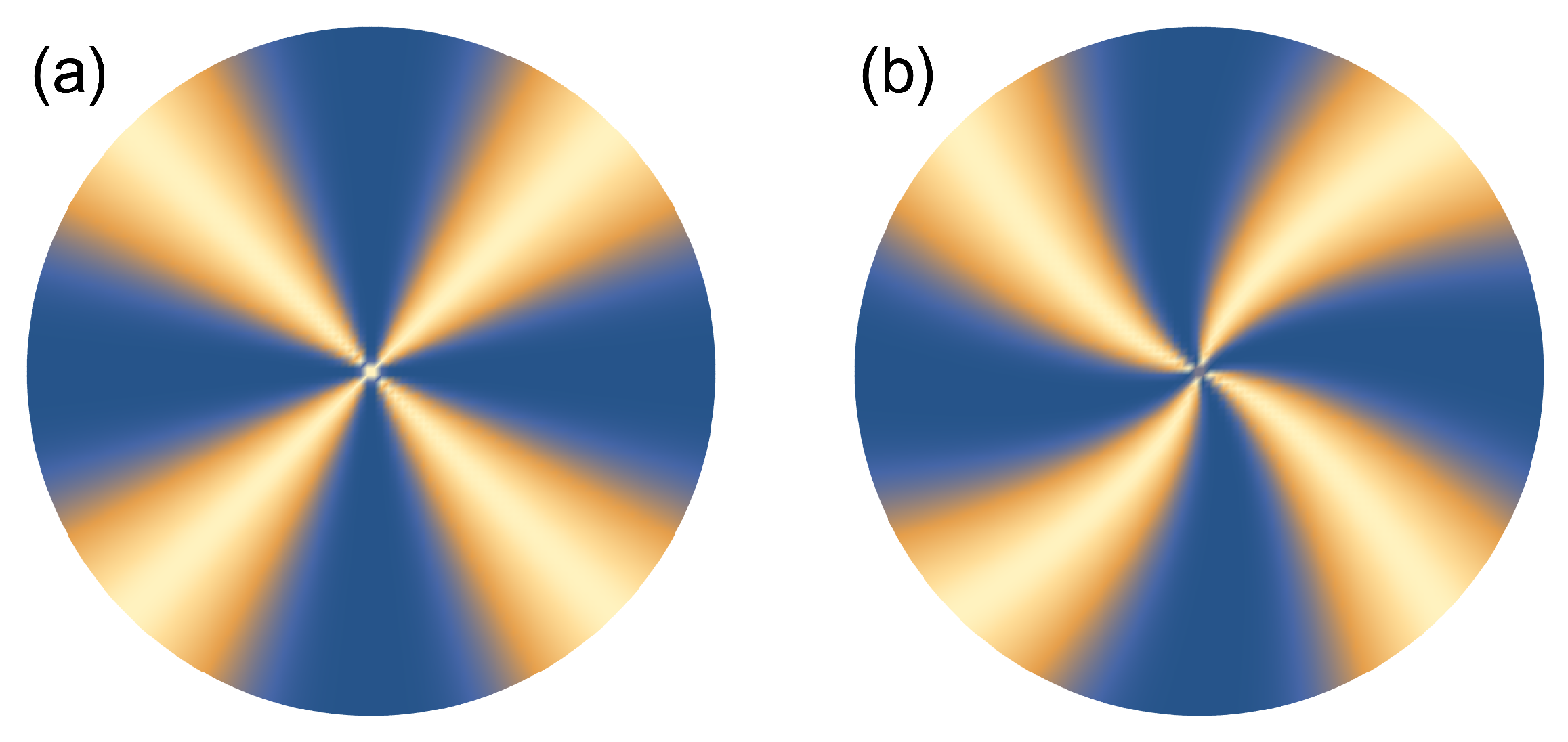
Computer generated images of (a) splay or bend defects and (b) spiral defects under crossed polarizers. The twisting or spiral structure is produced by a combination of splay and bend. The spiral structure was calculated with and corresponding to the orange curve in Figure 9.
Figure 2.
Computer generated images of (a) splay or bend defects and (b) spiral defects under crossed polarizers. The twisting or spiral structure is produced by a combination of splay and bend. The spiral structure was calculated with and corresponding to the orange curve in Figure 9.

Figure 3.
Phase diagrams for an annulus with (a) tangential and (b) perpendicular BCs. The dividing line between the two defect types is in (a) and in (b). In (a), the bend (spiral) defect is stable, and in (b), the splay (spiral) defect is stable in the shaded (unshaded) areas.
Figure 3.
Phase diagrams for an annulus with (a) tangential and (b) perpendicular BCs. The dividing line between the two defect types is in (a) and in (b). In (a), the bend (spiral) defect is stable, and in (b), the splay (spiral) defect is stable in the shaded (unshaded) areas.

Figure 4.
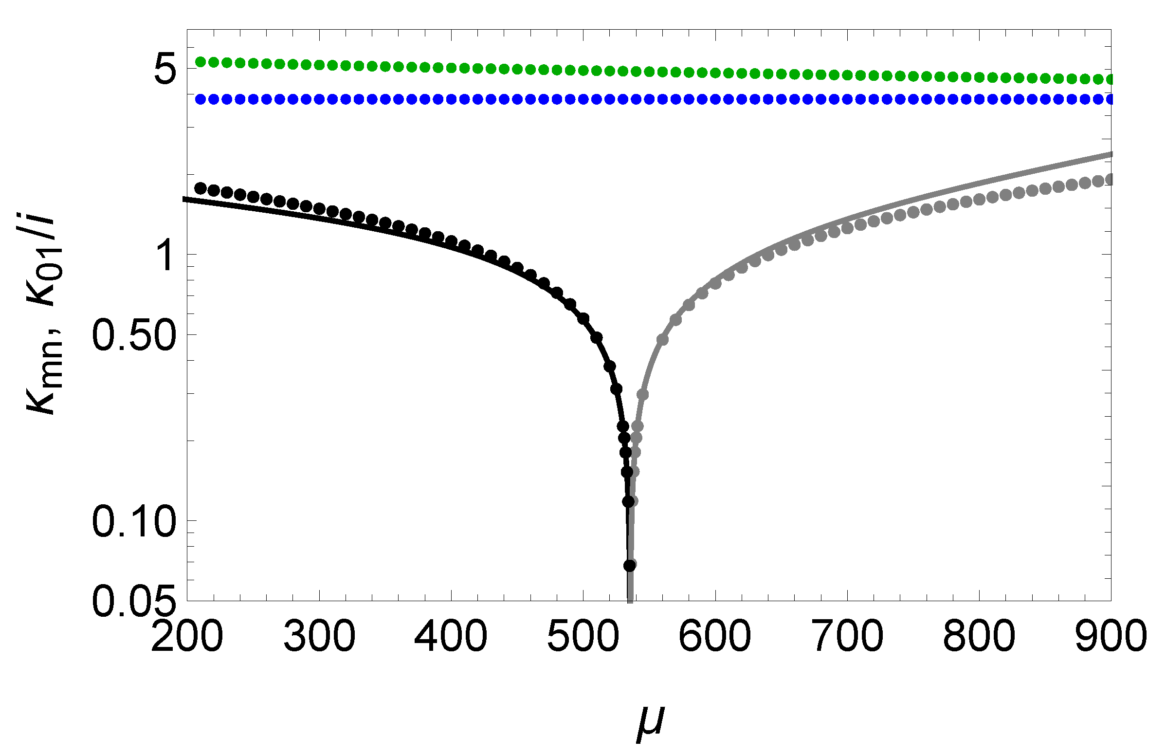
Wavenumbers as a function of for our sample configurations with imaginary and . The dots are obtained by numerical calculation of the zeros (black), (gray) and (blue) of the full function . The black line stems from our approximate analytical solution for as given in Equation (20). Note the excellent agreement between the black dots and the black line for close to . Also note the steep rise of the near .
Figure 4.
Wavenumbers as a function of for our sample configurations with imaginary and . The dots are obtained by numerical calculation of the zeros (black), (gray) and (blue) of the full function . The black line stems from our approximate analytical solution for as given in Equation (20). Note the excellent agreement between the black dots and the black line for close to . Also note the steep rise of the near .

Figure 5.
The radial eigenfunctions , where m and n are, respectively, the standard integer azimuthal and radial quantum numbers for polar coordinates, for a system with the imaginary value of used in Figure 6c. All plots are for , the lowest permitted value for n. On the ordinate, we included a factor , where is the total area enclosed by the outer circle of the trap so that the plotted eigenfunctions are dimensionless.

Figure 6.
The functions as a function of for , and : (a) for , (b) for ; (c) for , and (d) as a function of for . The rapid oscillations are a consequence of the logarithmic scale. Note that there are no zeros at small for (a,b) indicating large values of both for cases with and for modes with (and greater). In addition, the positions of the zeros in (a,b) are fairly insensitive to the value of and to the critical point. In (c), there is a zero in the top curve () that vanishes at and ceases to exist for . In (d), there is a zero in bottom curve () that vanishes at and then disappears when . has an infinity of larger-value zeros in (c), whereas in (d), it has only one zero when .

Figure 7.
The correlation function defined in Equation (34). The left shows the correlation as a function of dimensionless coordinates in the plane. The green loop indicates an assumed probing radius of . The right shows a zoom-in on the correlation function along the green loop.
Figure 7.
The correlation function defined in Equation (34). The left shows the correlation as a function of dimensionless coordinates in the plane. The green loop indicates an assumed probing radius of . The right shows a zoom-in on the correlation function along the green loop.

Figure 8.
Plots of calculated from Equation (37) as a function of for different values of . Note, grows exponentially as approaches 1, and the regions depicted in this figure are relative to a large value of for small .
Figure 8.
Plots of calculated from Equation (37) as a function of for different values of . Note, grows exponentially as approaches 1, and the regions depicted in this figure are relative to a large value of for small .

Figure 9.
Plot of for mixed states with and for different values for : (red), (blue), and (orange). Note the peak in amplitude near the core.
Figure 9.
Plot of for mixed states with and for different values for : (red), (blue), and (orange). Note the peak in amplitude near the core.

Publisher’s Note: MDPI stays neutral with regard to jurisdictional claims in published maps and institutional affiliations. |
© 2021 by the authors. Licensee MDPI, Basel, Switzerland. This article is an open access article distributed under the terms and conditions of the Creative Commons Attribution (CC BY) license (https://creativecommons.org/licenses/by/4.0/).
Share and Cite
MDPI and ACS Style
Stenull, O.; Lubensky, T.C. Director Fluctuations in Two-Dimensional Liquid Crystal Disclinations. Crystals 2022, 12, 1. https://0-doi-org.brum.beds.ac.uk/10.3390/cryst12010001
AMA Style
Stenull O, Lubensky TC. Director Fluctuations in Two-Dimensional Liquid Crystal Disclinations. Crystals. 2022; 12(1):1. https://0-doi-org.brum.beds.ac.uk/10.3390/cryst12010001
Chicago/Turabian StyleStenull, Olaf, and Tom C. Lubensky. 2022. "Director Fluctuations in Two-Dimensional Liquid Crystal Disclinations" Crystals 12, no. 1: 1. https://0-doi-org.brum.beds.ac.uk/10.3390/cryst12010001
Note that from the first issue of 2016, this journal uses article numbers instead of page numbers. See further details here.