
Characterization of Thickness Loss in a Storage Tank Plate with Piezoelectric Wafer Active Sensors

1
Safety Monitoring and Intelligent Diagnosis Laboratory, College of Safety and Ocean Engineering, China University of Petroleum (Beijing), Beijing 102249, China
2
CNPC Research Institute of Safety & Environment Technology, Beijing 102200, China
3
Key Laboratory of Optoelectronic Technology and System of Ministry of Education, College of Optoelectronic Engineering, Chongqing University, Chongqing 400044, China
*
Author to whom correspondence should be addressed.
Crystals 2022, 12(1), 92; https://0-doi-org.brum.beds.ac.uk/10.3390/cryst12010092
Submission received: 23 November 2021
/
Revised: 31 December 2021
/
Accepted: 2 January 2022
/
Published: 10 January 2022
(This article belongs to the Special Issue Piezoelectric Sensors Application)
Abstract
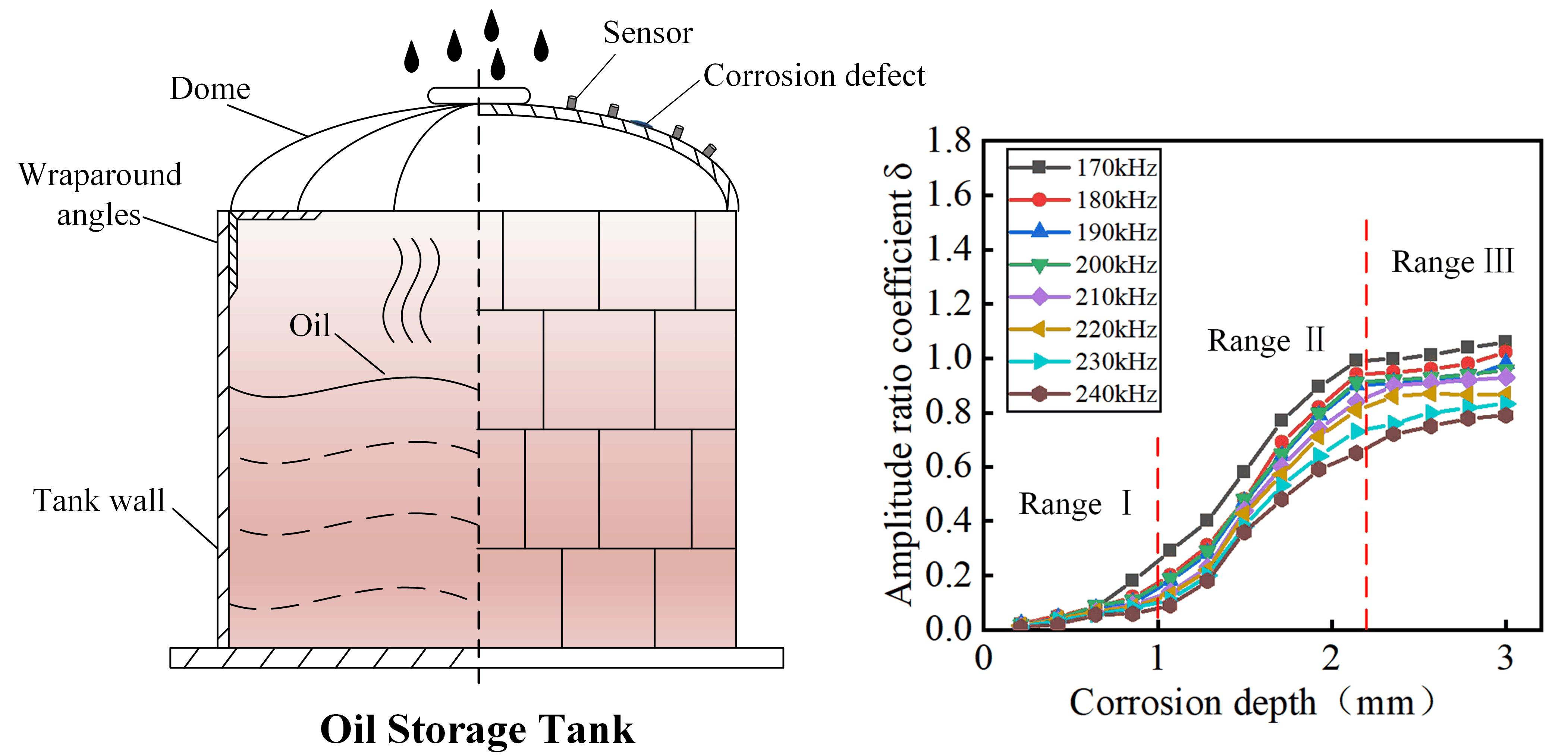
:In terms of the structural health inspection of storage tanks by ultrasonic guided wave technology, many scholars are currently focusing on the tanks’ floor and walls, while little research has been conducted on storage tank roofs. However, the roof of a storage tank is prone to corrosion because of its complex structure and unique working environment. For this purpose, this paper proposes a reflection/transmission signal amplitude ratio (RTAR) coefficient method for corrosion depth assessment. We studied the relationship between the RTAR coefficient, the corrosion depth, and the guided wave frequency to establish a depth assessment model. More importantly, unlike the traditional reflection coefficient method, the characteristics of guided wave signals, including the propagation and attenuation, are introduced in this model for accurate assessment. To eliminate the interference of residual vibration and improve the detection accuracy of defects, we built a corrosion detection system by using piezoelectric sensors and carried out field tests to verify the performance of the proposed method. We demonstrate that corrosion defects with a minimum depth of 0.2 mm can be quantitatively evaluated.
1. Introduction
Corrosion causes wall thinning in storage tanks, which leads to failures and leakage of the tanks. The leakage of a storage tank may have many serious consequences, such as severe casualties and property losses [1,2,3]. Various nondestructive testing (NDT) methods are widely used to inspect storage tanks, such as magnetic particle inspection, radiographic inspection, Eddy current inspection, acoustic emission inspection, and ultrasonic inspection [4,5]. However, the inspection of corrosion on the tank’s roof is challenging. In many tank structures, the fragility of the roof, the hazards linked to the inspection environment, the inaccessibility of corrosion defects, and the limitations of remote inspection can make it inefficient to assess [6,7,8,9,10,11]. Therefore, the goal of this study is to develop an ultrasonic inspection technique applicable to tank tops for the depth quantification of corrosion defects considering the propagation attenuation factor.
Since ultrasonic guided waves can propagate over long distances in thin-walled structures, and monitoring locations can obtain waveform signals containing defect information, several ultrasonic inspection techniques have been proposed for tank health assessment in the last few years [12,13]. Some papers have focused on the detection and characterization of corrosion defects using ultrasonic guided waves, which mainly studied the wave field and energy changes when guided waves interact with defects. Gao H et al. [14,15] studied the wave field energy change process caused by the corrosion defect damage on a thin aluminum plate by using finite element method (FEM) simulation tools and located the corrosion defect according to the energy change value. Fromme et al. [16,17] proposed using high-frequency guided wave technology to detect corrosion defects and found a correlation between the defect depth and the amplitude beat length. Yu et al. [18] used piezoelectric wafer active sensors (PWAS) for damage localization imaging with array signal processing on various thicknesses of plate specimens. The received signals from the electromagnetic acoustic transducer (EMAT) arrays that encircled the pipe were processed using computerized ultrasonic tomography to generate maps of the thickness loss [19,20]. Douka et al. [15,16] evaluated crack depth and defined an intensity factor that relates the wavelet coefficients to crack depth.
The mentioned methods mainly study the corresponding relationship between a certain characteristic of ultrasonic guided waves and the degree of corrosion defects, while less attention has been paid to the influencing factors in the actual application process, such as the influence of corrosion defects, the relative spatial distance, and the guided wave excitation signal frequency. These factors have a great influence on the detection results. Thus, the evaluation parameters and quantitative research on the depth of corrosion defects under different relative distances and excitation frequencies need to be studied in-depth.
Following this introduction, a statement on the inspection principle of corrosion depth is given in Section 2. It includes a theoretical analysis of the Lamb wave dispersion equation, selection of the Lamb wave frequency, and the principle of the RTAR coefficient method. In Section 3, the effects of relative distance and excitation frequency on the propagation characteristics of guided waves at different corrosion depths are studied by finite element simulation. Then, we build a corrosion detection system using piezoelectric active sensors and carry out field tests to verify the performance of the method. Finally, some conclusions are drawn in Section 4.
2. Inspection Method of Corrosion Depth
2.1. Lamb Wave Dispersion Equation
The elastic stress wave of a Lamb wave in an infinite plate belongs to the free plate problem. The solution to the problem of Lamb wave propagation in the plate satisfies the equation of motion (1) and the boundary condition (2), as follows:
where μ, λ, and ρ are the Lamb constant, wave number, and density of the plate material, respectively. And u is the displacement of the stress field. According to the above equations, the characteristic frequency Equation (3) of the Lamb wave vibration form in the plate can be further derived. The function is related to the plate thickness, frequency, wave number, etc.
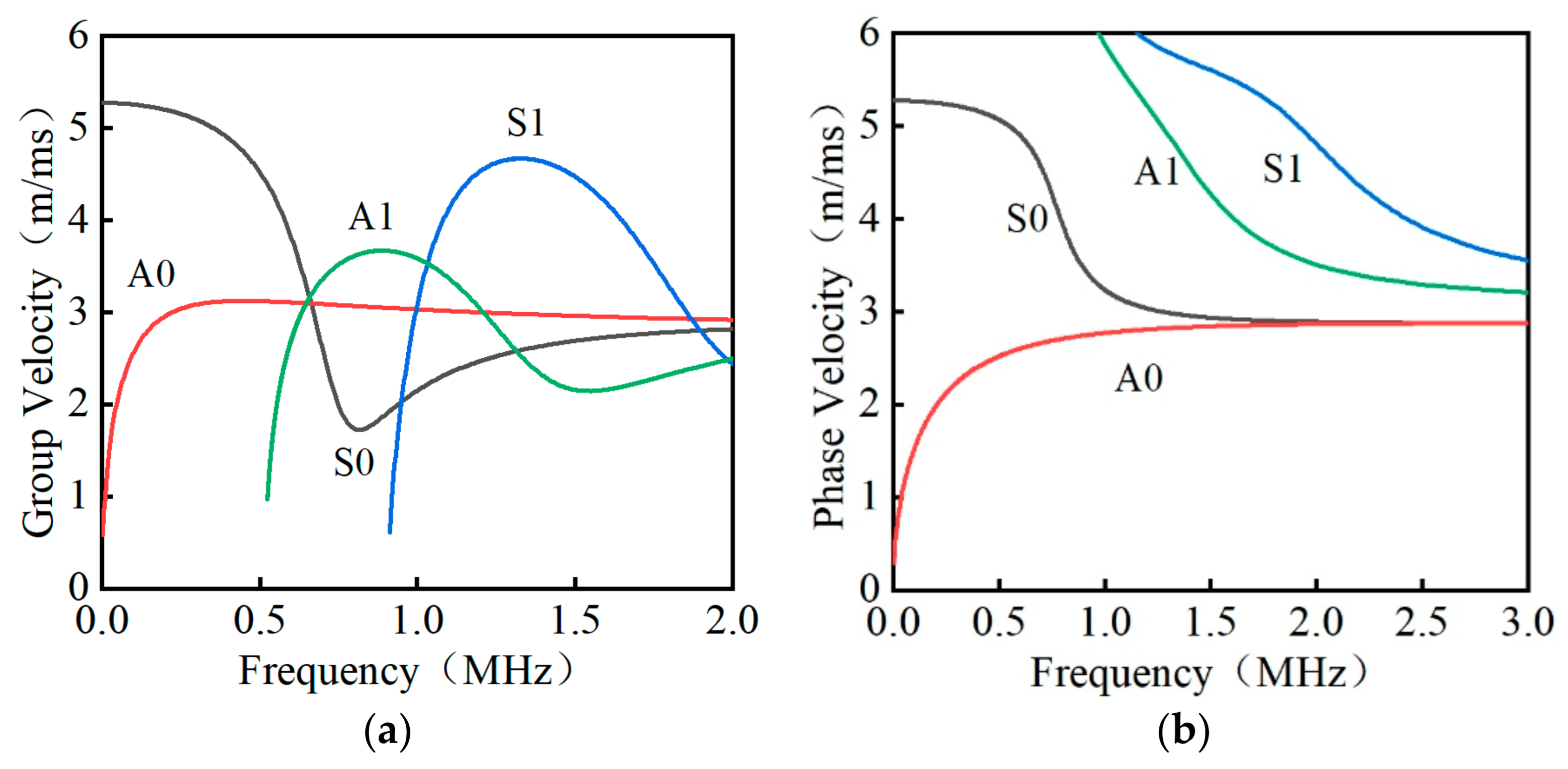
In the above equations, , where is the wave number, is the longitudinal wave speed, is the transverse wave speed, is the frequency, and h is the plate thickness. The above equations reflect the multimodal and dispersive characteristics of the Lamb wave. Lamb wave modes are roughly divided into two modes: the Symmetry Lamb wave (S mode) and the Antisymmetric Lamb wave (A mode). The dispersion curves reveal the nonlinearity between the wave number k and the frequency ω. This research mainly focuses on the quantitative evaluation of the corrosion defects of storage tanks. To simulate the on-site test conditions, a Q235 steel plate with a thickness of 3 mm is selected for constructing an experimental platform. The transverse wave velocity in the plate is 3100 m/s, and the longitudinal wave velocity is 5900 m/s. The relationship curve is calculated using the Disperse software, as shown in Figure 1.
2.2. Selection of the Lamb Wave Frequency
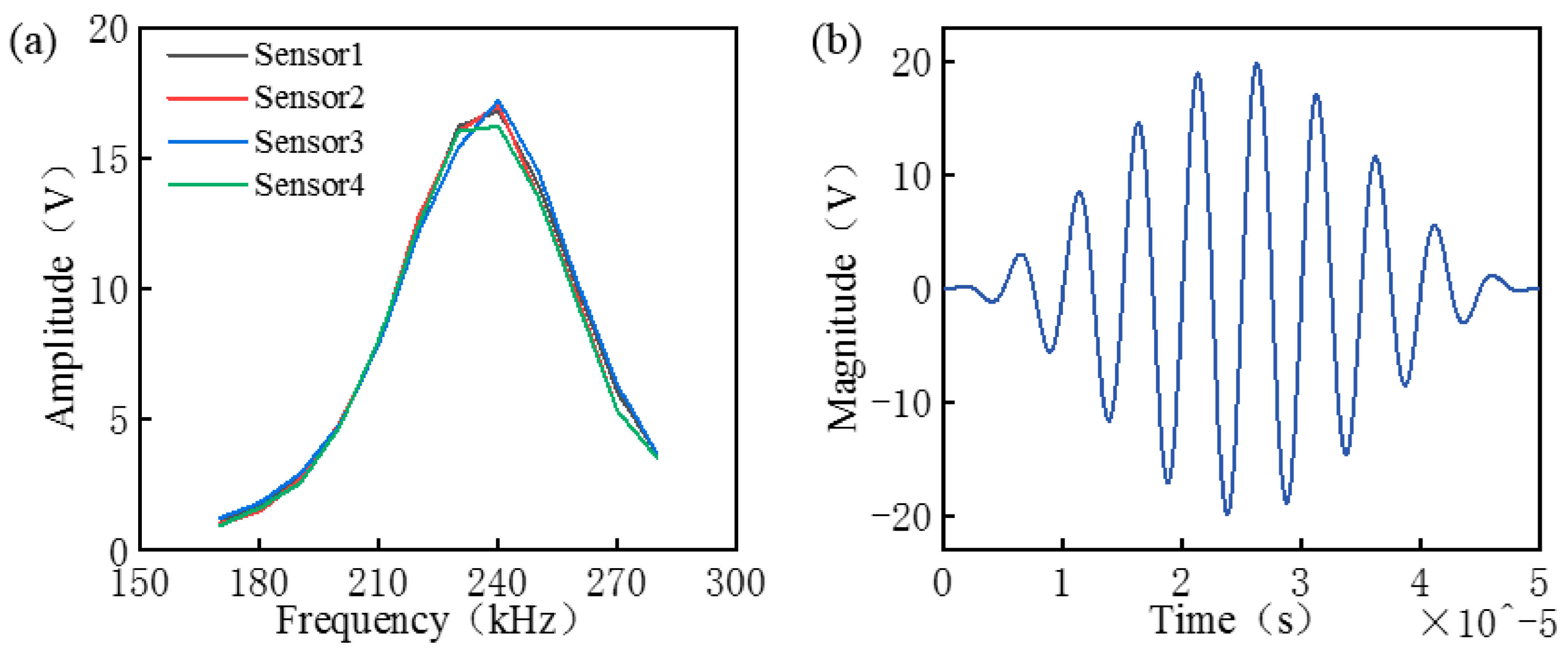
Theoretically, signal processing is easier and more accurate when there are fewer modes. The dispersion curve is shown in Figure 1. There are at least two modes in the steel plate at any frequency, making signal analysis difficult. It is found that A0 mode is more sensitive to the depth change of corrosion defects, so A0 mode is selected in the experiment. To ensure the accuracy of the experiment, the piezoelectric active transducer with a diameter of 20 mm is tested and the results show that the transducer performs best at about 240 kHz (see Figure 2). The frequency curves of multiple receiving sensors are also tested and the sensors showed good consistency (see Figure 2). In the experiment, a voltage signal with an amplitude of 20 V and 10 Hanning windows is used as the excitation source signal.
2.3. Reflected/Scattered Wave Amplitude Ratio (RTAR) Coefficient Method
Corrosion defects change the rigidity of a plate structure. When ultrasonic guided waves pass through defects, they are reflected, transmitted, and modally converted due to deformation and discontinuous boundary in the medium. When the depth and location of the corrosion defects change, the amplitude of the scattered wave will change accordingly. To accurately detect the corrosion depth, the attenuation caused by the amplitude and the propagation distance should be considered. Therefore, in this study, the RTAR coefficient is defined as the evaluation parameter. As mentioned in Section 2.1, an ultrasonic transducer is used to excite the ultrasonic guided wave at a point of the structure. The dispersion characteristics of the guided wave in the propagation process are considered. Assuming that the position of the transducer is the zero point in the time-space domain, the displacement component along the x-axis of the incident wave is as follows [21]:
The first term, , represents the wave propagating along the positive direction of the x-axis; the second term, , represents the wave propagating along the negative direction of the x-axis; and and .
The wave directly incident on the defect position in a single direction is considered; the displacement of the incident wave can be expressed as:
In this case, the displacement of the reflected echo and of the transmitted wave at any point in the time-space domain can be expressed as:
The sound attenuation in gas-solid two-phase media can be classified into three types according to the following loss mechanisms: geometric spreading, material damping, and wave scattering. This study mainly considers the geometric spreading of the plate-like structure. The function of the amplitude with the propagation direction and location L is fitted as the following equation:
where is the peak amplitude of the incident wave, L is the distance from the excitation source along the propagation direction, and is the peak amplitude of the wave packet from the excitation source L in the x-direction.
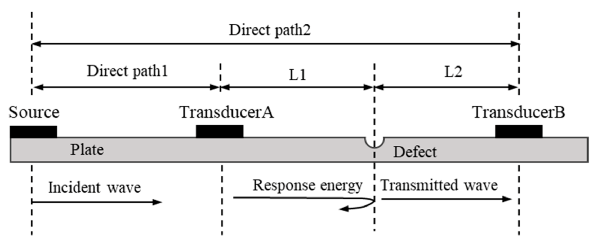
The propagation diagram, assuming that the position of the defect is the zero point in the time-space domain, is shown in Figure 3. When the incident wave propagates along the propagation direction and encounters the defect, due to the discontinuity of the medium, wave reflection, transmission, and the scattering phenomenon will occur. According to the principle of conservation of energy, the sum of the reflected wave energy at the defect, the transmitted wave energy at the defect, and the scattered wave energy at the defect constitute the total energy at the defect. For the specific guided wave mode propagating in the slab structure, combined with Equations (6)–(8), the reflected wave amplitude at the receiving point Transducer A at the distance from the defect , and the transmitted wave amplitude at the receiving point Transducer B at the distance from the defect , can be expressed as:
where is the reflected wave packet amplitude of the incident wave at the defect, and is the transmitted wave packet amplitude of the incident wave at the defect. Under the same frequency, the energy of the reflected wave and the transmitted wave is only related to the location of the receiving sensor. The ratio coefficient δ of the reflected signal to the transmitted signal amplitude at the defect is defined as:
where is defined as the attenuation factor of the guided wave propagation. δ is determined by the propagation distance of the reflected wave and the projected wave. The distances and between the receiving point and the defect in Equation (10) can be obtained from the wave-time information of the measured data. This equation is suitable for corrosion defect detection at any relative distance.
3. Results and Discussion
3.1. Finite Element Analysis
A three-dimensional FEM model of a steel plate with a corrosion defect is built by using the commercial FEM software ABAQUS. The dimensions of the steel plate are 600 mm × 600 mm × 3 mm, and the steel plate has three elements through the plate thickness. An element size of 1 × 1 × 1 mm3 is used; and the time step is 0.0003 s, which meets the required stability conditions in the space iteration and time convergence criteria in the finite element solution process. To eliminate boundary effects, two 80 mm-wide absorbing boundaries are placed along the edges of the model. To study the changes in the reflection and transmission signals of the propagation field caused by the depth of the defect, the corrosion defect is located at the center of the steel plate. The area of the corrosion is 20 mm × 20 mm, and the corrosion depth is set as 0.6 mm, 1.5 mm, 2.2 mm, and 3.0 mm. The material properties of the steel plate used in the simulations are listed in Table 1.
The excitation sinusoidal pulse modulated by the Hanning window has 10 cycles. Considering the frequency band of the sensor and the plate thickness, the center frequency of the excitation signal ranges from 170 to 240 kHz. At the same time, we consider the attenuation characteristics of the guided wave, the reflection distance , and the transmission distance changed. As a result, the propagation attenuation factor β of the guided wave becomes , 1, and , 1.
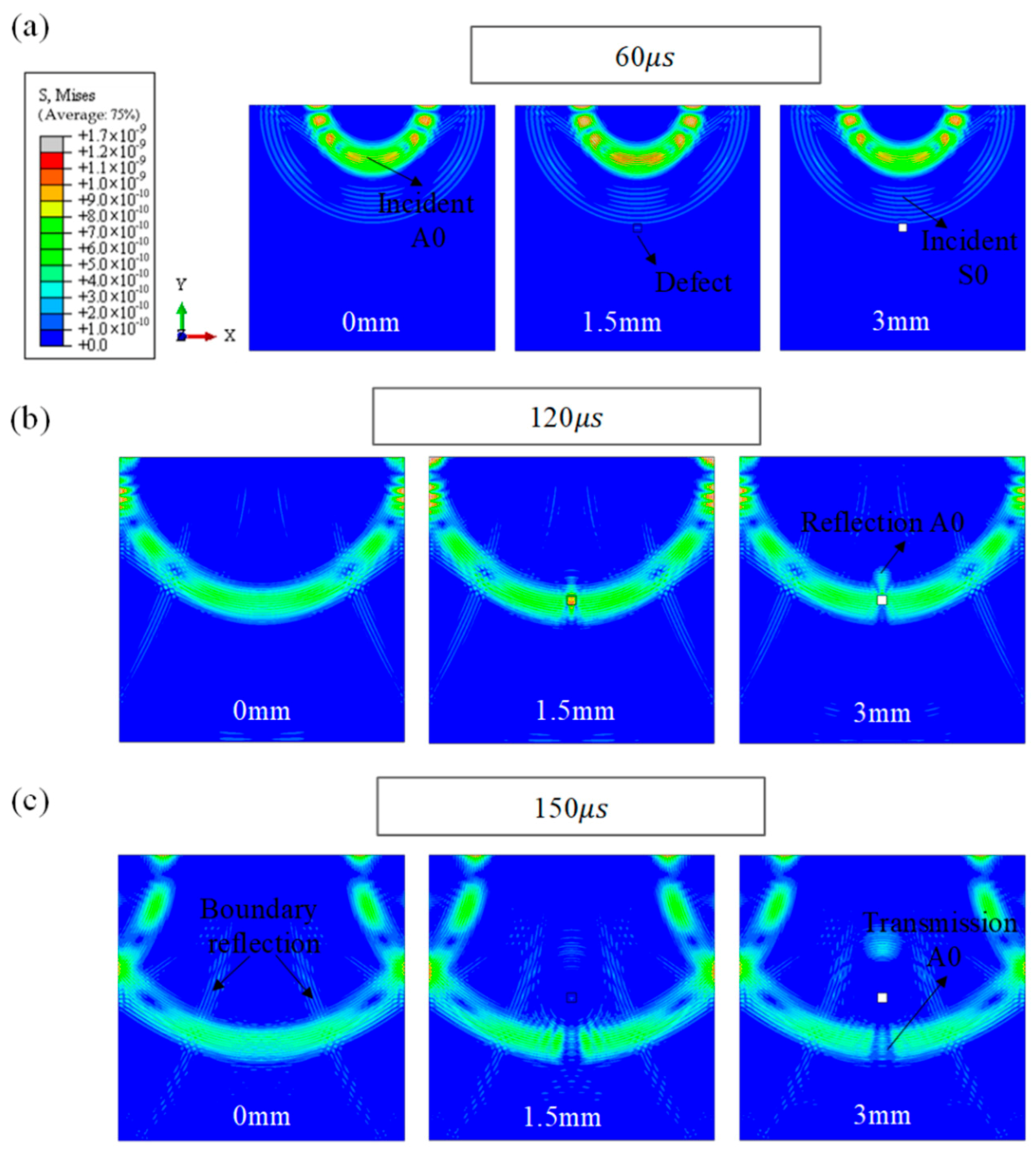
Figure 4 shows the numerical simulation results for the time evolution of the displacement contour in the z-direction during the simulated guided wave signal propagation in the corrosion plate when f = 200 kHz and h = 0 mm, 1.5 mm, and 3 mm. The displacement contours in Figure 4 visually show the effect of the corrosion depth on the guided wave signals. The simulated guided wave signal spreads around initially. After interacting with the corrosion, the mode conversion occurs, which generates the scattered waves, as shown in Figure 4b,c. These scattered waves continue to propagate and are received by the receivers along with the reflected waves from the edges. When the corrosion depth in the plate changes, so do the reflected wave magnitude and the transmitted wave magnitude generated by the interaction of the waves with the defect. Despite the complexity of wave propagation, it should be strongly emphasized that the color of A0 is darker than that of S0, which indicates that the A0 mode has a larger proportion in the propagation.
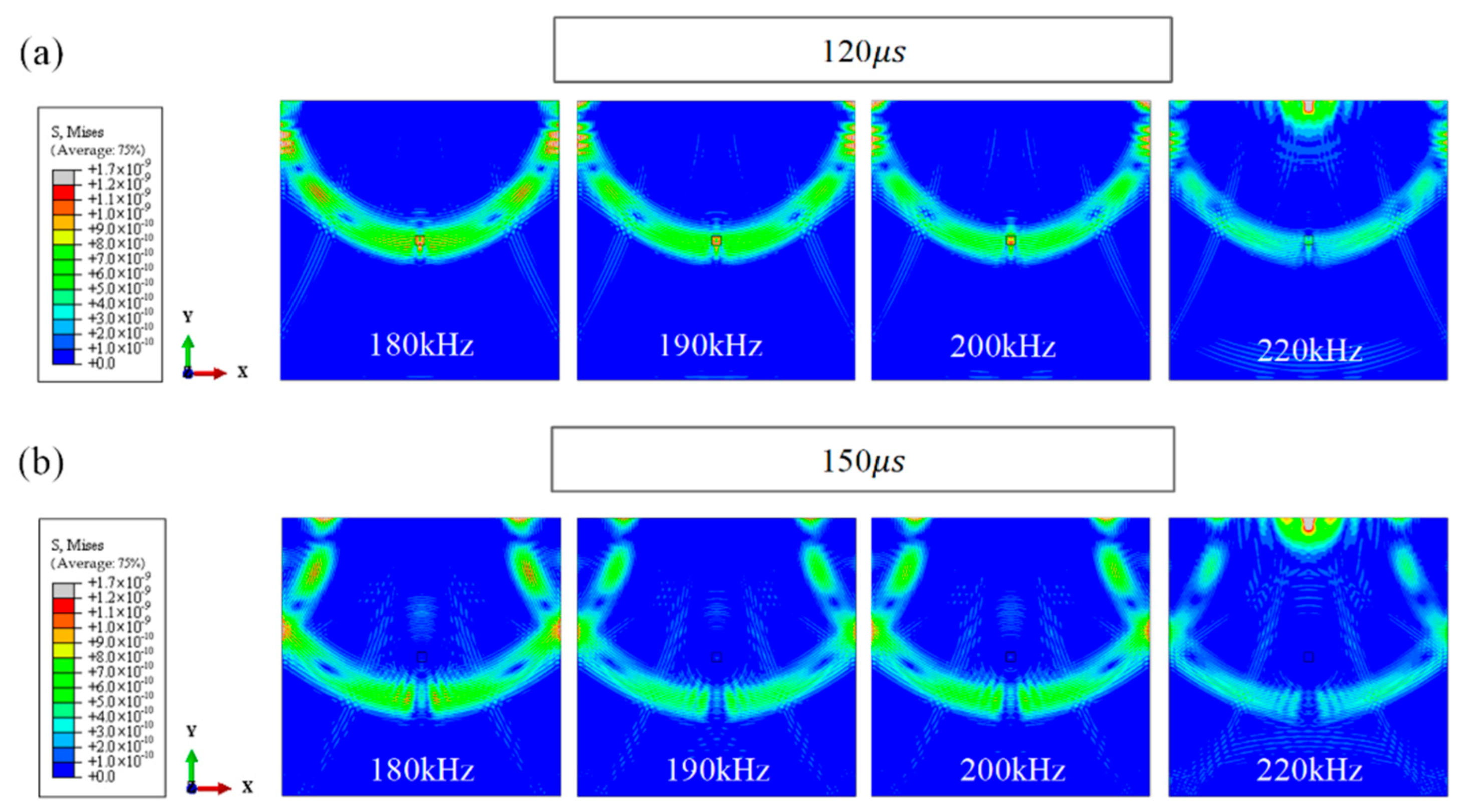
With the defect depth set at 1.5 mm, the wave propagating under normal excitation with different guided wave signal frequencies are used for numerical analysis, as shown in Figure 5. At the excitation frequency of f = 180 kHz–220 kHz, two guided wave modes are present, the S0 and A0 modes. The A0 mode is significantly slower than the S0 mode and the A0 mode is much more dispersive than the S0 mode. The wave scatters from the corrosion defect become apparent at t = 120 s, with clear mode conversion at t = 150 s. When the other conditions are maintained, the change in the excitation frequency makes the magnitude of the transmitted wave A0 unequal. The waves that have already been reflected or transmitted from the edges of the corrosion are captured by the receiving points.
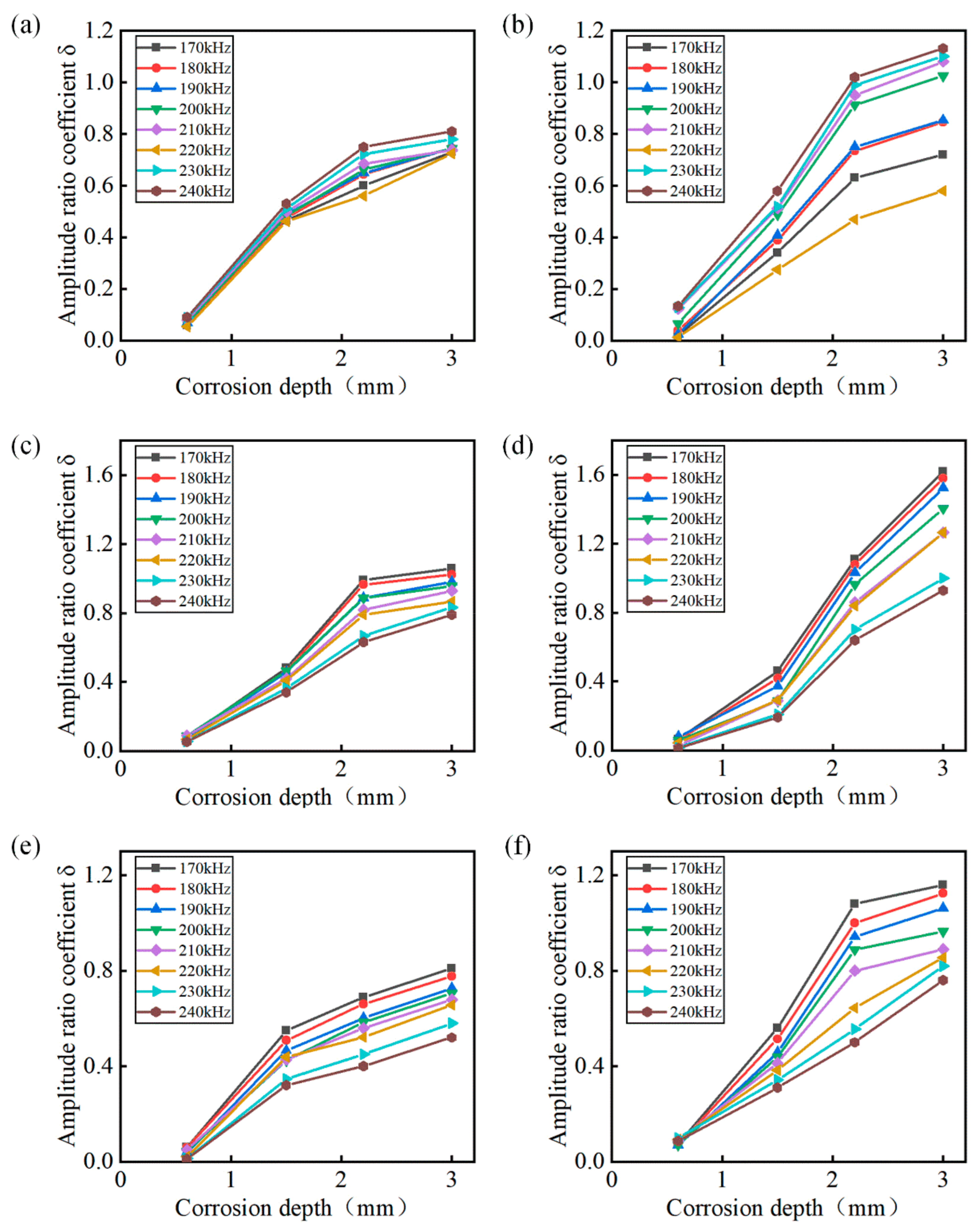
The relative positions of the corrosion defect and the reflected and transmitted difference of the attenuation factor β will cause the change of the amplitude ratio factor δ. Meanwhile, both the frequency of the excitation signal and the depth of the defect being detected have an impact on the guided wave detection capability. Therefore, to study the guided wave propagation attenuation and the reflected and transmitted wave amplitude ratio, the relationship between the amplitude ratio of the reflected and transmitted wave and the depth of the corrosion defect under different attenuation factors β and excitation frequencies f are investigated, as shown in Figure 6. It can be seen from Figure 6 that under different excitation frequencies f, the amplitude ratio coefficient δ of the defects is positively correlated with the defect depth. The smaller the excitation frequency f is, the larger the amplitude ratio coefficient δ under the same defect depth is. Moreover, when the corrosion depth h is the same as the attenuation factor β, the larger the values of and are, the smaller the defect amplitude ratio coefficient δ is. By determining the ratio of attenuation of the guided wave propagation and the frequency of the excitation signal, the corresponding corrosion defect depth can be obtained according to the defect depth to amplitude ratio curve, so the degree of corrosion of the defect can be obtained.
3.2. Corrosion Depth Detection Experiment Piezoelectric Wafer Active Sensor
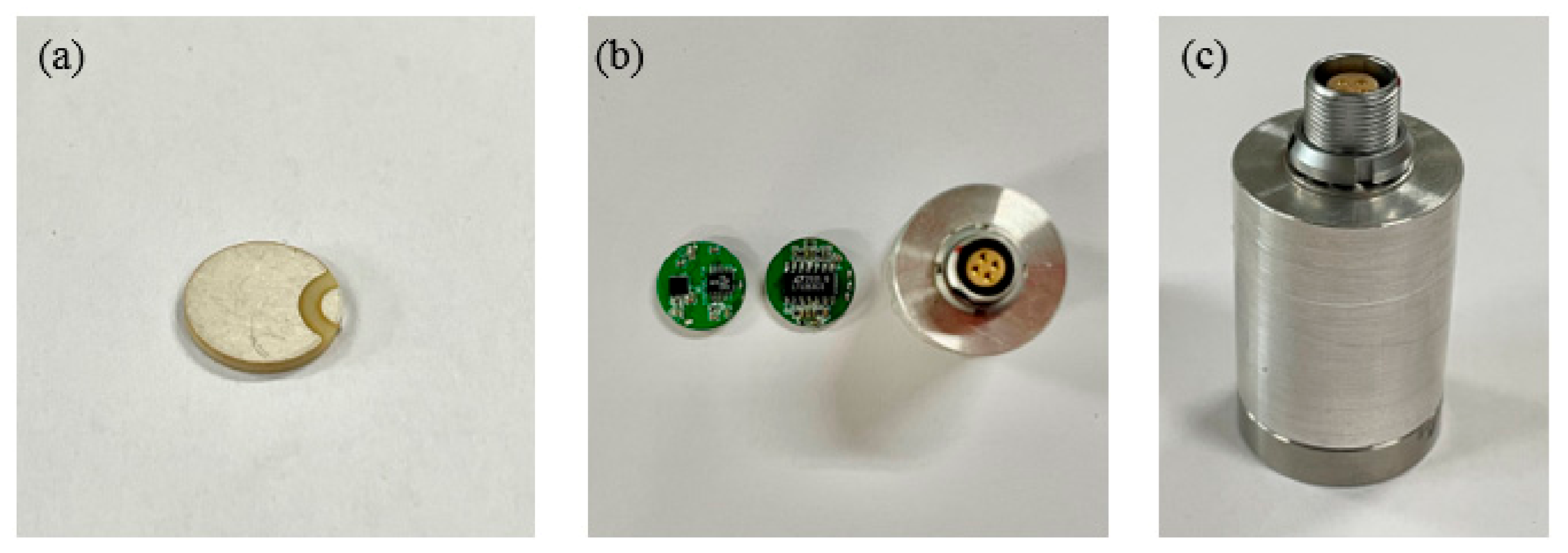
The RTAR coefficient method applies to the roof of a storage tank. The stored substances in oil storage tanks can produce flammable and explosive, corrosive gases or liquids, so precision instruments entering the oil area must be of explosion-proof design. At the same time, residual vibrations of the piezoelectric sheet will seriously affect the accuracy of corrosion defect depth detection. Therefore, home-made piezoelectric active sensors with explosion-proof design were developed. Typically, a sensor mainly includes a Φ10 × 1 mm piezoelectric ceramic sheet, a matching layer, a backing layer, filter amplifier circuits, and a stainless-steel shell. Among them, the piezoelectric ceramic sheet was the core functional material responsible for converting acoustic signals to electrical signals. The main function of the matching layer is to improve the energy conversion efficiency of the piezoelectric ceramic sheet, and its thickness is 1/4 of the wavelength of the sound wave signal of the frequency selected in the experiment. The role of the backing layer is to effectively avoid the interference caused by residual vibration. The filter amplifier circuits filter the received signal as well as performs power amplification to achieve a final voltage amplification effect of 10 times. Therefore, in the experiment, the Al2O3 ceramic chip is selected as the matching layer material of the home-made sensor, and tungsten powder and epoxy resin were mixed at a ratio of 10:1 as the backing material, with the material parameters shown in Table 2. The physical picture of the sensor probe is shown in Figure 7.
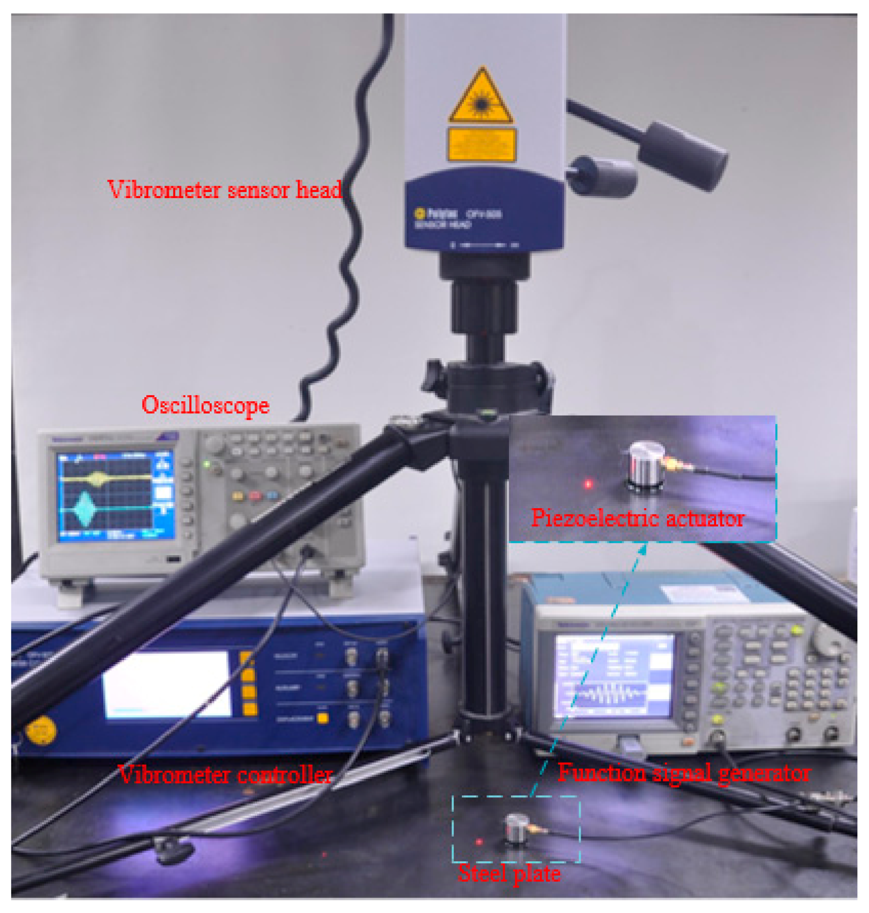
The home-made sensors were calibrated to ensure consistent sensor performance. Polytec’s OFV single-point laser vibrometer was used to measure the vibrational velocity of the steel plate quickly and precisely under the excitation of the piezoelectric vibration source (FUJICERA, AE144S). In the laser vibrometer, a single point vibrometer sensor head (Polytec, OFV-505) was used to receive the laser reflection signal from the measured position; while the vibrometer controller (Polytec, OFV-5000) connected with the sensor head was responsible for decoding the laser reflection signal into the vibrational velocity based on laser doppler vibration measurement technology. The vibrational velocity was displayed and recorded by an oscilloscope (Tektronix, TBS1102). The experimental arrangement is shown in Figure 8, with the excitation and reception positions spaced 20 mm apart, the excitation signal frequency at 170 kHz–240 kHz, and the excitation voltage at 10 V. The home-made sensor sensitivity curve is shown in Figure 9.
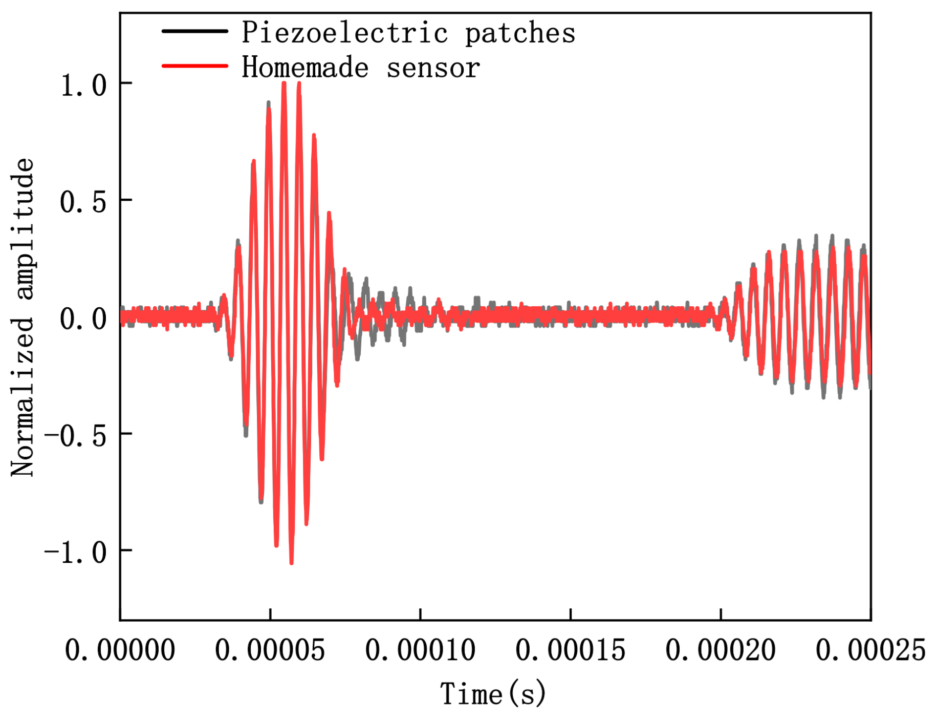
Under the excitation of the same commercial sensor (AE503S acoustic emission sensor produced by Fujifilm), the piezoelectric ceramic sheet and the packaged sensor were used to receive the guided wave signal and normalize the received signal. Figure 10 shows the comparison of the excitation signal of the piezoelectric wafer before and after assembly. The residual vibration of the piezoelectric sheet significantly improved after assembly, which was conducive to the subsequent experiments.
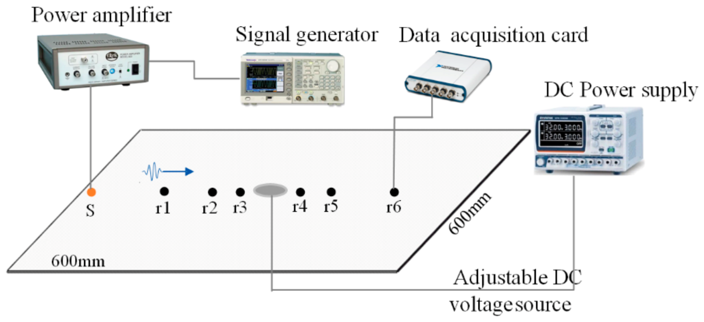
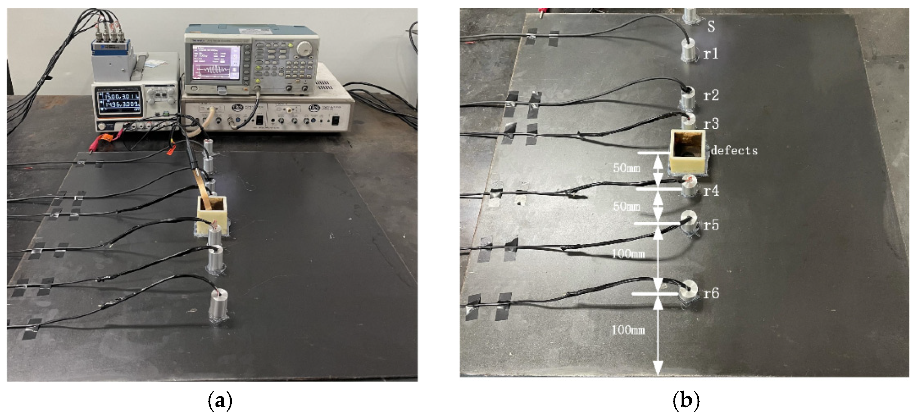
Figure 11 shows the experimental setup of the corrosion depth measurements, an ultrasonic guided wave signal generator, a power amplifier, a data acquisition card, and an adjustable direct current (DC) voltage source. Under electrical excitation, the excitation sensor generated guided waves in the steel plate. The guided waves propagated with an out-spreading pattern, were attenuated due to the damping of the material, underwent reflection and transmission through defects, and finally, were captured by the receiving sensors. The sample was made of a 600 600 3 mm Q235 steel plate. The excitation and receiving sensors were arranged as shown in Figure 10; the excitation transducer was located on the midpoint of one side of the steel plate, and the receiving transducers could be placed around the feature to receive waves through the plate by using a linear configuration of receiving transducers array. The amplitude ratio coefficients under different guided wave propagation attenuation factors β were obtained by arranging r1–r6 receiving transducers, which agreed with the simulation results. The excitation signal adapted a 10-period sine signal modulated by a Hanning window, and the frequency range was 170–240 kHz.
A corrosion formation test was carried out using the impressed current technique. Specifically, the steel plate served as the cathode, the copper sheet acted as an anode, and a 3.5% solution of sodium chloride (NaCl) was poured as an electrolyte into a corrosive vessel to form an electrolytic cell. A power supply equipped with a built-in ammeter and potentiometer was used to impress a DC to the steel plate to induce its significant corrosion in a short period. A constant voltage of 15 V was maintained across the solution and the specimen until the steel plate was corroded and perforated. To measure the data at different corrosion depths with uniform variation, waveform signals were acquired for every 10 min of corrosion using a data acquisition card. Figure 12 shows the experimental platform for performing depth detection of corrosion defects.
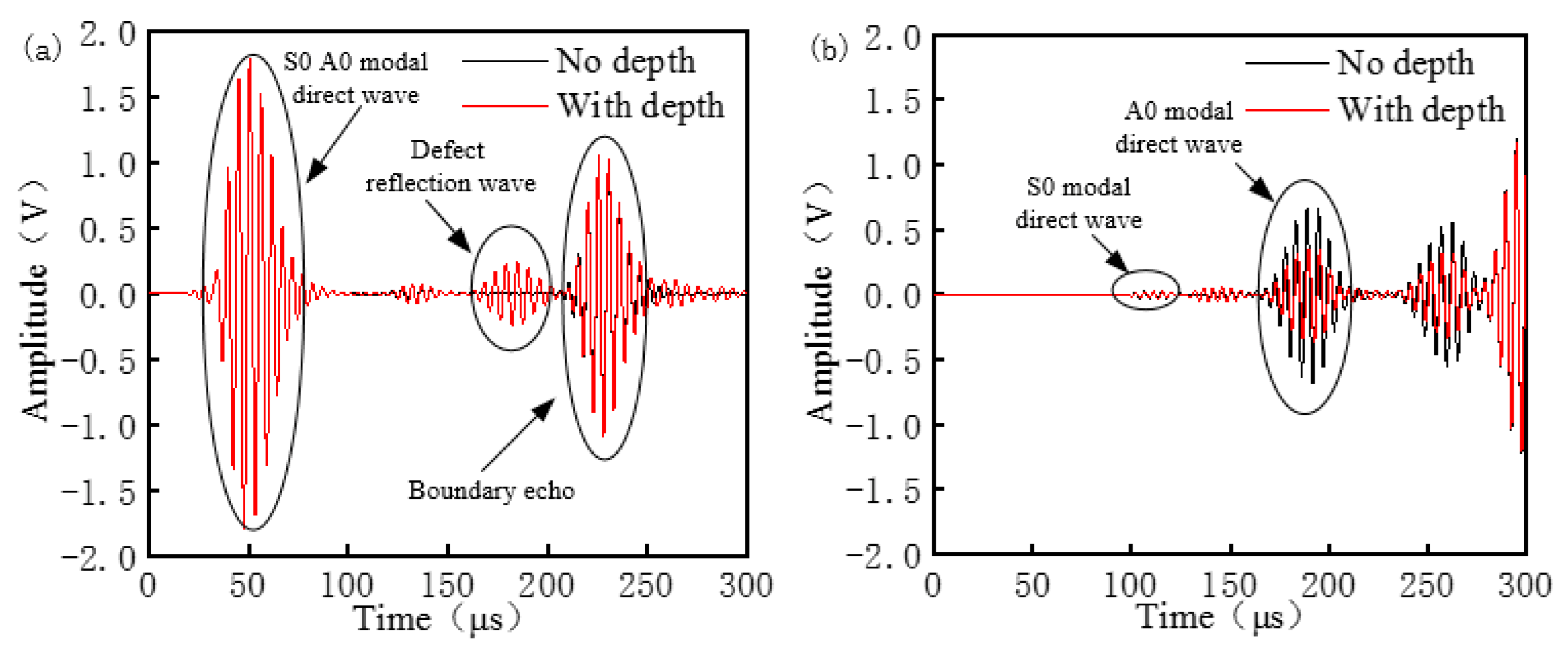
Figure 13a,b show the reflected and transmitted wave signals received by sensor r1 and sensor r6, respectively. The excitation signal voltage was 30 V and the excitation frequency was 200 kHz. From Figure 13a, it can be seen that the received signal in the waveform mainly existed as a direct wave, a defective reflected wave, and a boundary echo. We found that the S0 and A0 modes were mixed, which, after analysis, was thought to be caused by the small spacing between S and r1. From the dispersion curve in Figure 1, we know that the wave speed of the S0 mode at 200 kHz was 5200 m/s, the wave speed of the A0 mode was 2700 m/s, and the duration of the excitation wave was 50 µs. It is known that the spacing between S and r1 is 100 mm, so the time for the S0 mode to reach r1 is 20 µs, and the time for the A0 mode to reach r1 is 38 µs. The time deviation between them is less than 50 µs. Therefore, the S0 waves and A0 waves overlap at r1. Similarly, in Figure 13b, it can be seen that there are mainly separated S0 mode waves, A0 mode waves, and boundary echoes in the received signal in the waveform. The time difference between the two is greater than 50 µs, so the S0 and A0 modes are distinguishable at the r6 position.
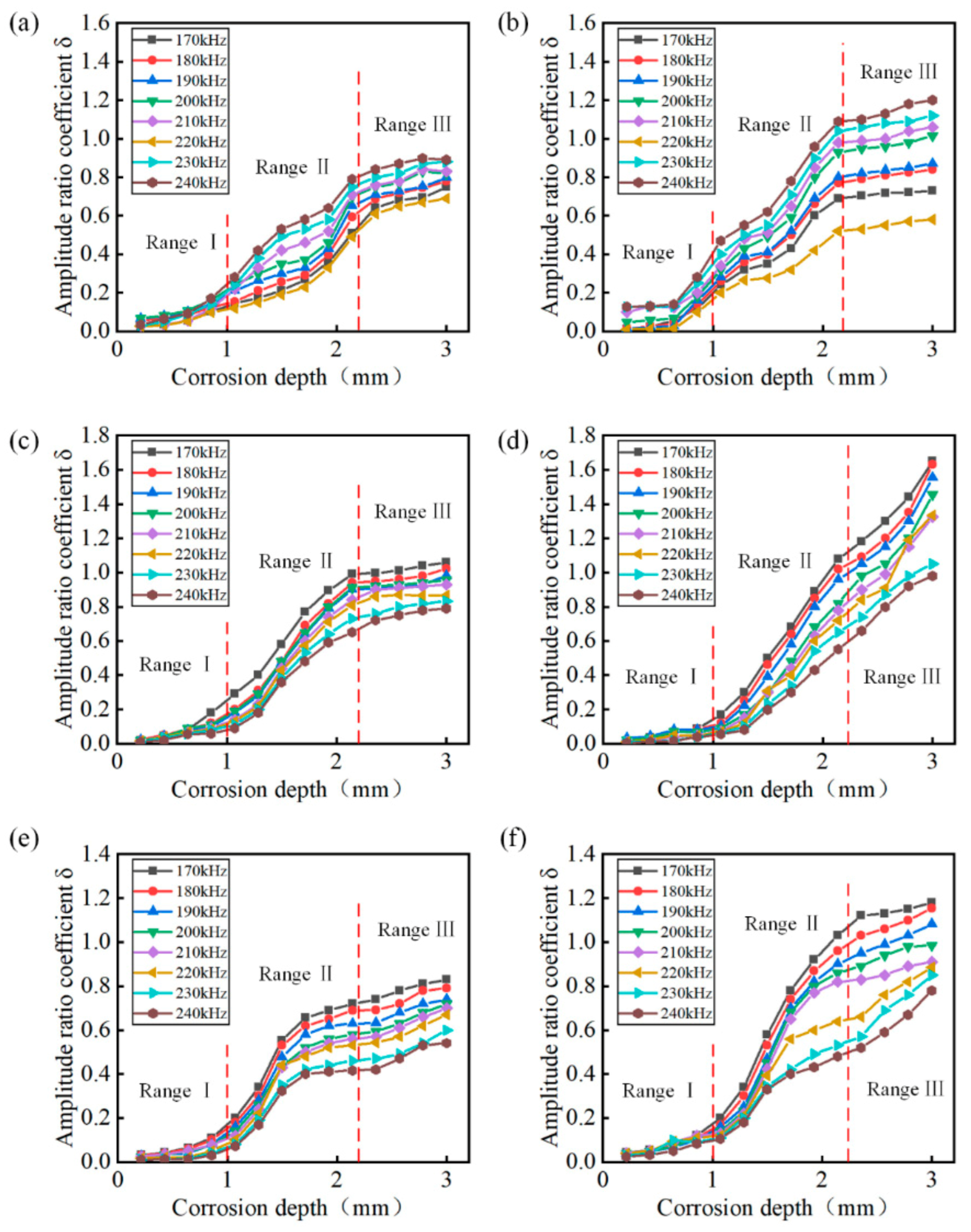
Figure 14 shows that the interaction with defects varied for the same attenuation factor β and the different distances when the excitation frequency was between 170 kHz and 240 kHz, as seen in the change curve between the coefficient δ and the corrosion defect depth. The amplitude ratio coefficient δ increased monotonically with the increased corrosion depth at almost all the excitation frequencies considered in this study. The corrosion process depicted in Figure 14a shows that when the 220 kHz signal was used, the amplitude ratio coefficient at the attenuation factor β = 1 and the / = 200/200 was at its lowest, which means that the 220 kHz signal is not ideal for the detection and evaluation of the defect depth. Figure 14b shows that when the 220 kHz signal was used, the amplitude ratio coefficient at the attenuation factor β = 1 and / = 100/100 was at its lowest. When the defect depth was the same, the amplitude ratio coefficient increases with an increase in the excitation frequency, except at the special frequency in Figure 14a,b. Figure 14c–f shows that when the depth of the corrosion defects was the same, the amplitude ratio coefficient decreased with an increase in the excitation frequency. The variation of the amplitude ratio coefficient with the frequency is a complex process since the waves’ interaction with the damage differs at different frequencies.
The amplitude ratio coefficient curves show that a square defect with a side length of 20 mm and a corrosion defect with a depth of 0.21 mm was detectable. Thus, a monotonic increment of the amplitude ratio coefficient with damage growth suggests that the damage can be monitored for a range of growth rates. The results of this study demonstrate how the amplitude ratio coefficient of a guided wave signal can be used in conjunction with the linear array concept at different frequencies to monitor corrosion and hole damages.
3.3. Application of RTAR Coefficient to Storage Tank
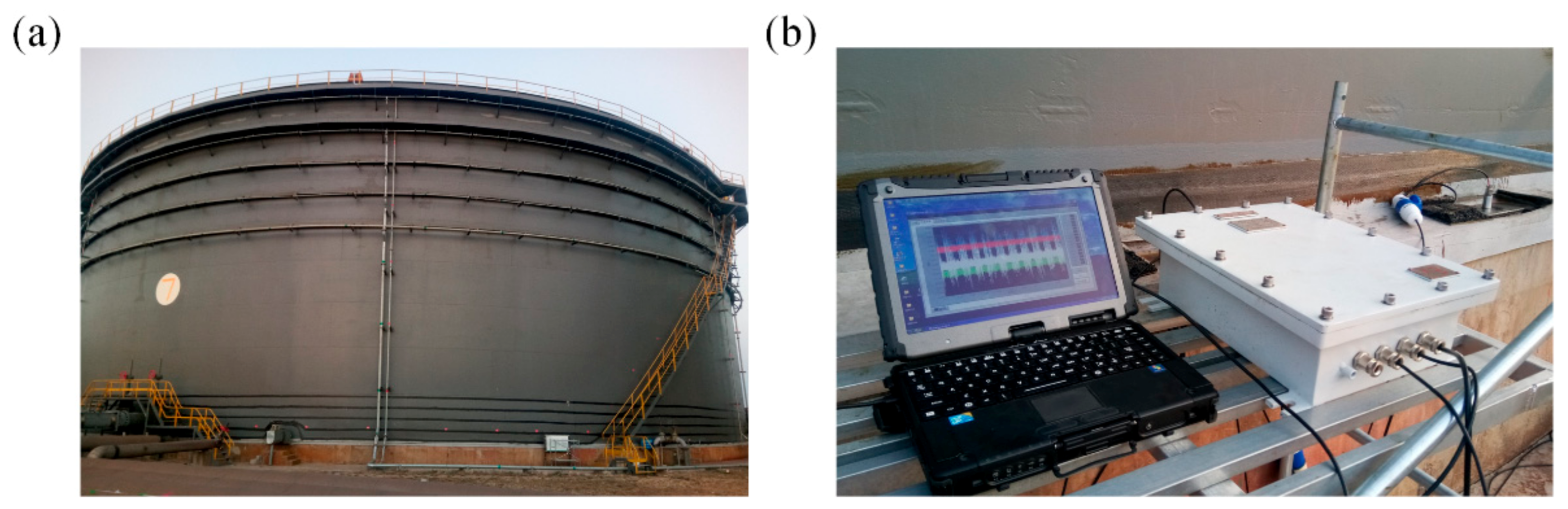
A 60 m-diameter storage tank was used to carry out the structural health monitoring experiments. The capacity of the entire tank was 50,000 m3. As guided waves have a high energy attenuation after long-distance transmission, it is difficult to obtain an accurately reflected wave signal. Therefore 36 sensors were fixed to the perimeter of the tank and arranged in a circular array. The self-developed available eight-channel active AE-structure health detector and an explosion-proof computer were used to collect the guided wave data of the tank roof. The transmitted waves collected by the circular sensor array were combined with a probabilistic damage imaging algorithm to achieve rough imaging of the tank roof defects. As the defect location was known in the probabilistic damage imaging map, a linear array of sensors was arranged within 1–2 m of a particular path through the defect. In combination with the methods in this paper, quantitative depth detection was performed. The structural health monitoring system of the storage tank and the storage tank roof is illustrated in Figure 15.
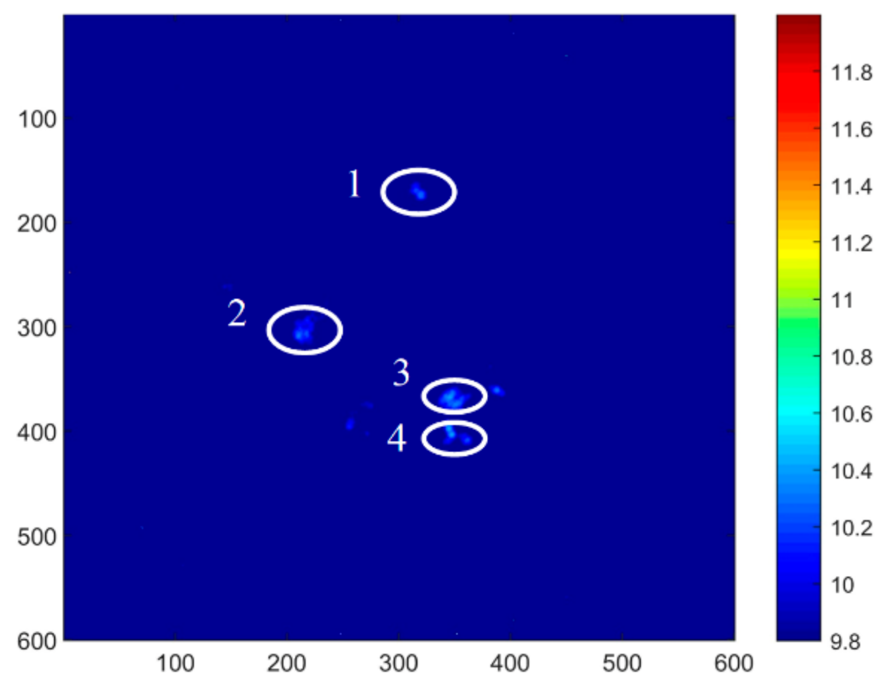
Figure 16 shows the images of the damage probabilities due to the corrosion in the storage tank roof. The images were collected during the field test. As shown in Figure 16, when the pixel value was larger than 10.1, the area was identified as a corrosion damage area. It was observed that the defects appeared in the white-circled zones. Table 3 shows the corrosion defect evaluation using the data collected from the field. The percentage error between the predicted corrosion depth and the actual corrosion depth was 6.7% for defect 1; 5.7% for defect 2; 2.2% for defect 3; and 6% for defect 4. Thus, the percentage error in monitoring shallow corrosion defects was higher than the percentage error in monitoring deep-depth corrosion defects under the same conditions.
The experiment results confirm that the proposed corrosion depth damage quantification method can accurately quantify the corrosion depth of storage tank roof structures.
4. Conclusions
In summary, we report a concept and experimental results based on the reflection/transmission amplitude ratio coefficient of corrosion defect depth detection. The growth of corrosion was monitored using the Lamb wave, and the damage probability imaging technique in the signal acquired by the linear array of sensors was used in the fast localization of damage. Then, parametric sensitivity for damages in a plate, such as corrosion growth and varying defect depth, were obtained in terms of the reflection and transmission amplitude ratio coefficient.
The corrosion depth detection experiment was performed through the measurement system. We found that the variation trend of the corrosion defect depth and the reflection/transmission amplitude ratio coefficient under different excitation frequencies were consistent with the simulation results. As a result, we verified the relationship between the defect depth and the amplitude ratio change curve. This provided a way for the efficient parametric estimation of corrosion growth and variation of defect depth with time. By changing the linear array to the circular array, other sensors in the circular array can be used to monitor the damage in other parts of the board, and the appropriate frequency can be selected to reduce the influence of the distance attenuation factor. The appropriate algorithm can be used to automatically solve the amplitude ratio coefficient to estimate the defect depth.
Author Contributions
Conceptualization, W.L., J.F. and J.Y.; methodology, W.L. and J.Y.; data curation, J.Y.; writing—original draft preparation, W.L.; writing—review and editing, W.L.; project administration, W.L.; funding acquisition, W.L. All authors have read and agreed to the published version of the manuscript.
Funding
This work is supported by the national key research and development program of China “Key technologies for performance testing and evaluation of high temperature and high pressure petrochemical pressure seals (2020YFB2008000)”, and the key project grant program of PetroChina Company Limited (Grant number 2019D-2312).
Institutional Review Board Statement
Not applicable.
Informed Consent Statement
Not applicable.
Data Availability Statement
The data that support the findings of this study are available from the corresponding author upon reasonable request.
Acknowledgments
The author would like to thank the support by the national key research and development program of China “Key technologies for performance testing and evaluation of high temperature and high pressure petrochemical pressure seals (2020YFB2008000)”, and the key project grant program of PetroChina Company Limited (Grant number 2019D-2312).
Conflicts of Interest
The authors declare no conflict of interest.
References
- Ma, J.Z.; Cui, J.L. Application status of on-line detection technology for in-service crude oil storage tank. Petrochem. Technol. 2020, 27, 5–6. [Google Scholar] [CrossRef]
- Zhang, Y.Y.; Li, D.S.; Zhou, Z. Baseline-free method for the evaluation of uniform corrosion based on ultrasonic guided waves. Vib. Shock. 2019, 38, 115–120. [Google Scholar] [CrossRef]
- James, I.C.; Cheng, C.L. A study of storage tank accidents. J. Loss Prev. Process Ind. 2006, 19, 51–59. [Google Scholar] [CrossRef]
- Han, W.L.; Jiang, L.L.; Liu, R.; Su, B.H.; Wang, Z.T. Current application status of on-line inspection technology for oil storage tanks in-service. Pet. Eng. Constr. 2019, 45, 1–4. [Google Scholar] [CrossRef]
- Zhou, Y.S.; Chen, P.; Ding, K.Q. Design and Development of Security Monitor and Early Alarming System of Floating Roof Tank. In Proceedings of the 2015 Far East Nondestructive Testing New Technology Forum, Zhuhai, China, 28–31 May 2015; pp. 575–578. [Google Scholar]
- Luo, F.W.; Ran, R.; Wang, L. Study on Corrosion Law of Large Crude Oil Storage Tank Floor and Risk-Based Inspection and Maintenance Technology. Corros. Sci. Technol. 2020, 19, 66–74. [Google Scholar] [CrossRef]
- Kenji, K.; Satoshi, I.; Hiroyasu, I.; Takashi, Y. Statistical Analysis on Corrosion of Oil Storage Tank Bottom Plate. Zairyo-to-Kankyo 2011, 51, 99–104. [Google Scholar] [CrossRef] [Green Version]
- Sosoon, P.; Shigeo, K.; Kenji, K.; Sigenori, Y.; Hiroaki, M.; Kazuyoshi, S. Development of AE Monitoring Method for Corrosion Damage of the Bottom Plate in Oil Storage Tank on the Neutral Sand under Loading. Mater. Trans. 2006, 47, 1240–1246. [Google Scholar] [CrossRef] [Green Version]
- Aljarah, A.; Vahdati, N.; Butt, H. Magnetic Internal Corrosion Detection Sensor for Exposed Oil Storage Tanks. Sensors 2021, 21, 2457. [Google Scholar] [CrossRef] [PubMed]
- Khalili, P.Y.; Cawley, P. The choice of ultrasonic inspection method for the detection of corrosion at inaccessible locations. NDT E Int. 2018, 99, 80–92. [Google Scholar] [CrossRef]
- Purwasih, N.; Shinozaki, H.; Okazaki, S.; Kihira, H.; Kuriyama, Y.; Kasai, N. Atmospheric Corrosion Sensor Based on Strain Measurement with Active–Dummy Fiber Bragg Grating Sensors. Metals 2020, 10, 1076. [Google Scholar] [CrossRef]
- Liu, Z.H.; He, C.F.; Wu, B.; Wang, X.Y. Hidden Corrosion Detection in Plate-like Structure using Lamb Waves. Exp. Mech. 2005, 20, 166–167. [Google Scholar] [CrossRef]
- Moon, S.; Kang, T.; Han, S.W.; Jeon, J.Y.; Park, G. Optimization of excitation frequency and guided wave mode in acoustic wavenumber spectroscopy for shallow wall-thinning defect detection. Mech. Sci. Technol. 2018, 32, 5213–5221. [Google Scholar] [CrossRef]
- Gao, H.; Guers, M.J. Flexible ultrasonic guided wave sensor development for structural health monitoring. In Proceedings of the Smart Structures and Materials + Nondestructive Evaluation and Health Monitoring, San Diego, CA, USA, 26 February–2 March 2006; pp. 61761I.1–61761I.12. [Google Scholar]
- Douka, E.; Hadjileontiadis, L.J. Time–frequency analysis of the free vibration response of a beam with a breathing crack. NDT E Int. 2004, 38, 3–10. [Google Scholar] [CrossRef]
- Masserey, B.; Fromme, P. On the reflection of coupled Rayleigh-like waves at surface defects in plates. J. Acoust. Soc. Am. 2008, 123, 88. [Google Scholar] [CrossRef] [PubMed]
- Masserey, B.; Fromme, P. High-frequency guided waves for defect detection in stiffened plate structures. Insight 2009, 51, 667–671. [Google Scholar] [CrossRef]
- Yu, L.; Victor, G. Multi-mode Damage Detection Methods with Piezoelectric Wafer Active Sensors. J. Intell. Mater. Syst. Struct. 2009, 20, 1329–1341. [Google Scholar] [CrossRef] [Green Version]
- Nurmalia; Nakamura, N.; Ogi, H.; Hirao, M. EMAT pipe inspection technique using higher mode torsional guided wave T (0,2). NDT E Int. 2017, 87, 78–84. [Google Scholar] [CrossRef]
- Matthew, C.; Matthew, F.; Steve, D. Circumferential guided wave EMAT system for pipeline screening using shear horizontal ultrasound. NDT E Int. 2017, 86, 20–27. [Google Scholar] [CrossRef] [Green Version]
- Joseph, L.R. Ultrasonic Waves in Solid Media; Cambridge University Press: Cambridge, UK, 2014; pp. 40–45. ISBN 9781107273610. [Google Scholar]
Figure 1.
Dispersion curves of Lamb waves in a 3 mm-thick steel plate. (a) Phase velocity and (b) group velocity.
Figure 1.
Dispersion curves of Lamb waves in a 3 mm-thick steel plate. (a) Phase velocity and (b) group velocity.

Figure 2.
(a) The frequency response test curve of the sensor, and (b) the 10-count tone burst modulated through a Hanning window at 200 kHz.
Figure 2.
(a) The frequency response test curve of the sensor, and (b) the 10-count tone burst modulated through a Hanning window at 200 kHz.

Figure 3.
Illustration of the wave field propagation of the Lamb wave and the defect interaction.

Figure 4.
The finite element analysis (FEA) results; the magnitudes of the 200 kHz wave that propagated around the corrosion at different time increments: 0 mm, 1.5 mm, and 3 mm. The color scale represents the von Mises stress: (a) 60 µs, (b) 120 µs, and (c) 150 µs.
Figure 4.
The finite element analysis (FEA) results; the magnitudes of the 200 kHz wave that propagated around the corrosion at different time increments: 0 mm, 1.5 mm, and 3 mm. The color scale represents the von Mises stress: (a) 60 µs, (b) 120 µs, and (c) 150 µs.

Figure 5.
The FEA results; the frequencies of the wave that propagated around the 1.5 mm-deep corrosion defect at different time increments: 180 kHz, 190 kHz, 200 kHz, and 220 kHz. The color scale represents the von Mises stress: (a) 120 µs and (b) 150 µs.
Figure 5.
The FEA results; the frequencies of the wave that propagated around the 1.5 mm-deep corrosion defect at different time increments: 180 kHz, 190 kHz, 200 kHz, and 220 kHz. The color scale represents the von Mises stress: (a) 120 µs and (b) 150 µs.

Figure 6.
The attenuation factor β and the distance ratio L1/L2 differed when the excitation frequency was between 170 kHz and 240 kHz, as shown by the change curve between the reflection and transmission amplitude ratio coefficient δ and the corrosion defect depth. (a) β = 1 and L1/L2 = 200/200. (b) β = 1 and L1/L2 = 100/100. (c) β = and L1/L2 = 200/100. (d) β = and L1/L2 = 100/50. (e) β = and L1/L2 = 100/200, (f) β = and L1/L2 = 50/100.

Figure 7.
Physical sensor drawing: (a) PZT disk; (b) filter amplifier circuits; (c) encapsulated sensor.
Figure 7.
Physical sensor drawing: (a) PZT disk; (b) filter amplifier circuits; (c) encapsulated sensor.

Figure 8.
Experimental setup for measuring the vibrational velocity of the steel plate under the excitation of the piezoelectric vibration source.
Figure 8.
Experimental setup for measuring the vibrational velocity of the steel plate under the excitation of the piezoelectric vibration source.

Figure 9.
Sensor sensitivity curves: (a) home-made sensor excitation signal, Polytec’s OFV single-point laser vibrometer reception signal; (b) AE144S excitation signal, home-made sensor, and Polytec’s OFV single-point laser vibrometer reception signal.
Figure 9.
Sensor sensitivity curves: (a) home-made sensor excitation signal, Polytec’s OFV single-point laser vibrometer reception signal; (b) AE144S excitation signal, home-made sensor, and Polytec’s OFV single-point laser vibrometer reception signal.

Figure 10.
Pre-package sensor and encapsulated sensor: time-domain waveform comparison.

Figure 11.
Experimental setup of the corrosion depth measurements.

Figure 12.
(a) Experimental setup; (b) Layout of the PZT sensor. (unit: mm)

Figure 13.
Comparison of the predicted waveforms with and without a depth effect at a voltage of 30 V and a frequency of 200 kHz: (a) reflection signal and (b) transmission signal.
Figure 13.
Comparison of the predicted waveforms with and without a depth effect at a voltage of 30 V and a frequency of 200 kHz: (a) reflection signal and (b) transmission signal.

Figure 14.
The attenuation factor β and the distance ratio L1/L2 differed when the excitation frequency was between 170 kHz and 240 kHz, as shown by the change curve between the reflection and transmission amplitude ratio coefficient δ and the corrosion defect depth. (a) β = 1 and / = 200/200. (b) β = 1 and / = 100/100. (c) β = and / = 200/100. (d) β = and / = 100/50. (e) β = and / = 100/200. (f) β = and / = 50/100.

Figure 15.
(a) Storage tank with a 60 m diameter. (b) Floating-roof tank structural health monitoring system.
Figure 15.
(a) Storage tank with a 60 m diameter. (b) Floating-roof tank structural health monitoring system.

Figure 16.
Damage probability images of the corrosion in the storage tank roof (1, 2, 3, and 4 are the defect regions).
Figure 16.
Damage probability images of the corrosion in the storage tank roof (1, 2, 3, and 4 are the defect regions).


Table 1.
Material properties.
| Material | E/(GPa) | ρ/(kg/m3) | |
|---|---|---|---|
| Steel | 210 | 0.3 | 7850 |
Table 2.
Sensor material parameters.
| Material | Thickness (mm) | Diameter (mm) | Density (kg/m3) | Velocity of Sound (m/s) |
|---|---|---|---|---|
| PZT-5 | 1 | 10 | 7800 | 4674 |
| Al2O3 | 4 | 8 | 3920 | 10,500 |
| Epoxy resin | — | — | 1100 | 2200 |
| Tungsten powder | — | — | 19,350 | 5200 |
| Stainless-steel | 5 | 22 | 1000 | 1500 |
Table 3.
Results of the corrosion defect evaluation using the data collected from the field.
| Defect No. | Actual Corrosion Depth (mm) | Predicted Corrosion Depth (mm) | Percentage Error | Corrosion Grade |
|---|---|---|---|---|
| 1 | 1.2 | 1.28 | 6.7% | Region I |
| 2 | 4.4 | 4.15 | 5.7% | Region II |
| 3 | 5.1 | 5.21 | 2.2% | Region III |
| 4 | 3.7 | 3.48 | 6% | Region II |
Publisher’s Note: MDPI stays neutral with regard to jurisdictional claims in published maps and institutional affiliations. |
© 2022 by the authors. Licensee MDPI, Basel, Switzerland. This article is an open access article distributed under the terms and conditions of the Creative Commons Attribution (CC BY) license (https://creativecommons.org/licenses/by/4.0/).
Share and Cite
MDPI and ACS Style
Liu, W.; Fan, J.; Yang, J. Characterization of Thickness Loss in a Storage Tank Plate with Piezoelectric Wafer Active Sensors. Crystals 2022, 12, 92. https://0-doi-org.brum.beds.ac.uk/10.3390/cryst12010092
AMA Style
Liu W, Fan J, Yang J. Characterization of Thickness Loss in a Storage Tank Plate with Piezoelectric Wafer Active Sensors. Crystals. 2022; 12(1):92. https://0-doi-org.brum.beds.ac.uk/10.3390/cryst12010092
Chicago/Turabian StyleLiu, Wencai, Jianchun Fan, and Jin Yang. 2022. "Characterization of Thickness Loss in a Storage Tank Plate with Piezoelectric Wafer Active Sensors" Crystals 12, no. 1: 92. https://0-doi-org.brum.beds.ac.uk/10.3390/cryst12010092
Note that from the first issue of 2016, this journal uses article numbers instead of page numbers. See further details here.