1. Introduction
Roller conveying is a necessary step to complete the rolling industrial production of metal plates. Currently, open rollers or closed rollers are widely used to transport metal plates in production lines. Magnesium alloy has the characteristics of lower heat capacity and lower thermal conductivity, which lead to the following two phenomena: (1) In the process of roller conveying without auxiliary heat, temperature changes are very easily created because the heat dissipation and temperature differences are produced in the width and thickness directions of magnesium alloy plates. (2) Lower thermal conductivity can easily lead to the emergence of local temperature-drop zones, resulting in uneven temperatures in magnesium alloy plates. These two phenomena affect the formability and yield of plates during rolling deformation. To minimize the temperature drops in magnesium alloy plates during the roller conveying process and to ensure that the plates remain at the required temperature for subsequent rolling deformation, the roller conveying step needs to have the technical characteristics of continuity without interruption, fast speed, and closed auxiliary heat transmission. In this case, when using the traditional methods involving contact-temperature measurement (such as using thermometer, point thermometer or other temperature measuring tools), it is difficult to track and detect the plate-temperature status in real time [
1,
2]. Therefore, the off-line prediction of plate temperature is particularly important.
During the open-roller conveying process, the heat transfer between the plate and its surrounding medium primarily involves heat conduction to the conveying roller, as well as convection and radiation with the surrounding air [
3]. According to the Newton cooling formula, thermal conduction heat dissipation is proportional to the contact area [
4]. Since the contact between the plate and the conveying roller is linear, the heat dissipation between them can be ignored [
5]. According to one report [
6], the heat-flux density per unit area of thermal radiation is proportional to the quartic difference between the absolute temperatures of the two radiation surfaces, and the heat-flux density per unit area of the thermal convection heat dissipation is proportional to the difference in temperature between the surrounding air and the plate. During the air-cooling process for conventional strip steel, there is a significant temperature difference between the strip and the surrounding air. As a result, convective heat transfer only contributes a small proportion to the overall heat dissipation. J. Q. Sun [
7] estimated the comprehensive heat-transfer coefficient during the air-cooling process of a steel plate by assuming the heat-transfer mode of the steel plate in the heat-retention panel to be based on radiation. The results worked well for the prediction of the temperature history. Thus, considering that the accurate measurement and calculation of convective heat dissipation are difficult, the effect of convective heat transfer on the temperature of the strip plate can be ignored when calculating the temperature drop caused by air cooling [
8]. However, compared with steel and aluminum plate and strip, magnesium alloy plates bear lower preheating temperatures (250~450 °C [
9]), resulting in smaller temperature differences between these plates and the air. In addition, the volume-specific heat of magnesium alloy is smaller, which makes the temperature of magnesium alloy more sensitive to heat change [
10]. Therefore, the air-cooling behavior of magnesium alloy plates is more intricate than that of conventional strip steel. It is necessary to fully consider the use of thermal radiation and convection to accurately solve the thermal changes in magnesium alloy plates during transportation. Obviously, the traditional air-cooling model of strip steel cannot accurately describe the cooling behavior of magnesium alloy plates [
11].
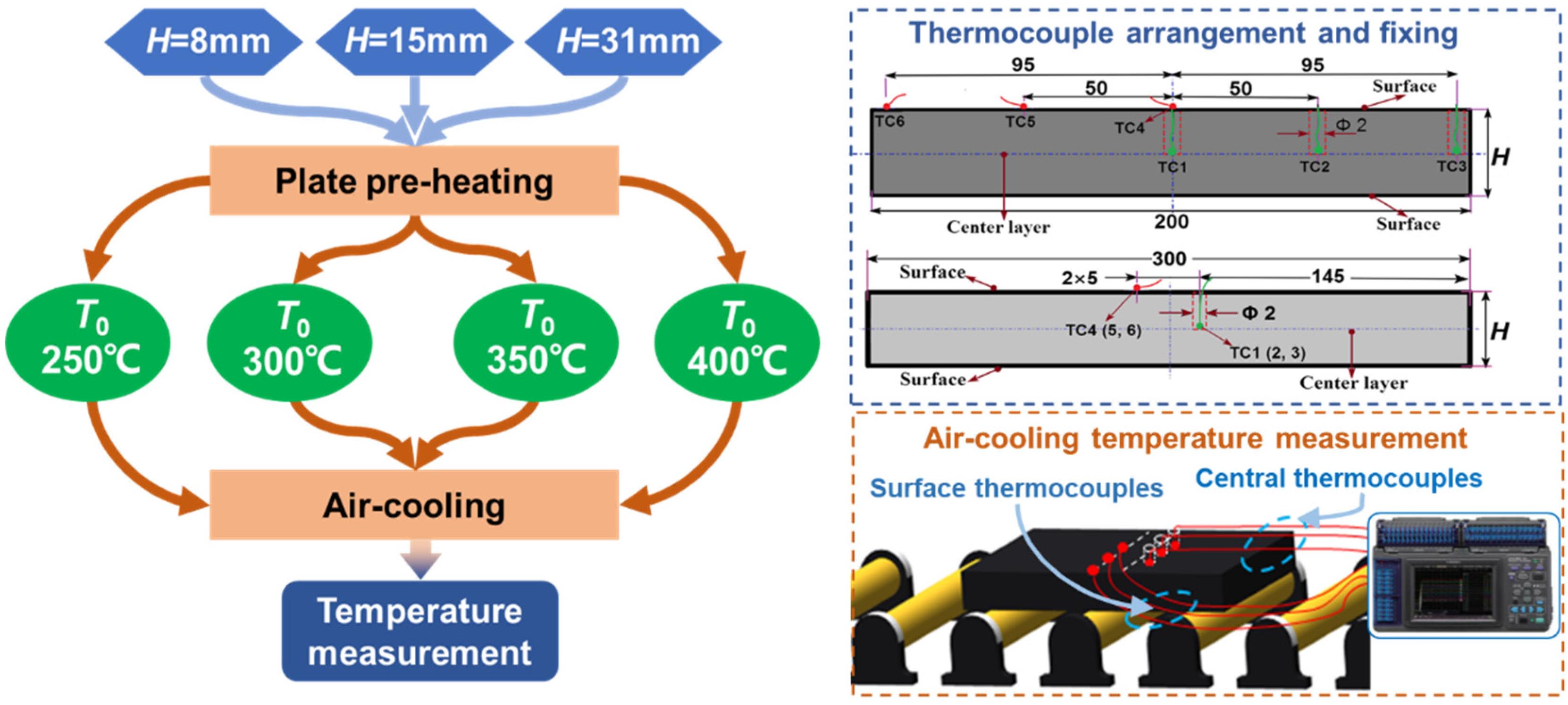
This study aims to build a temperature model for the AZ31B alloy plate air-cooling process, taking into account the comprehensive effects of thermal radiation and convection heat dissipation. The real-time heat-dissipation temperature drop of the plates was tested. The method of “discrete and dimension reduction solution, combination of temperature drop in two directions” was used to establish a three-dimensional temperature-distribution model for the magnesium alloy plate during non-auxiliary heat-roller transportation. Finally, the prediction accuracy of the model was verified by the real-time temperature-measurement data for the AZ31B magnesium alloy plate. The model can provide an important basis for temperature control and auxiliary heat implementation in the conveying process, which is of great significance for improving the forming quality of wide magnesium alloy plates.
3. Temperature Distribution and Evolution in Width and Thickness Directions
By calculating the temperature difference between the middle and the edge (
, Equation (1)) and difference in temperature between the surface and middle layers of the thickness (
, Equation (2)), a quantitative evaluation was conducted on the distribution characteristics of temperature in terms of plate thickness and width during the air-cooling process. The larger the value, the greater the temperature difference and the higher the degree of temperature non-uniformity.
Taking the air-cooling process of 15-mm- and 31-mm-thick slabs at initial temperatures of 250 °C and 400 °C as an example,
Figure 2 and
Figure 3 show the variation in
and
, respectively, over time. The B-splines (basic splines) were used for data-smoothing purposes. It can be seen from the figure that the change curves with time under the conditions of different plate thicknesses (15 mm, 31 mm) and different initial temperatures (250 °C, 400 °C) showed obvious unimodal characteristics, while the appearance of the peak value meant the generation of the maximum temperature gradient between temperature-measurement positions. The width-direction peak occurred at 150~200 s of air cooling, while that of the thick direction occurred at 140~185 s. The times of occurrence under the same conditions were approximately the same. For the pre-peak stage, the main heat-transfer mechanisms were the heat radiation and convection heat transfer from the slab to the air. In the width direction, because the edge had a greater air-contact area, the temperature drop at the edge was greater than that at the middle, resulting in a sharp increase in the width-direction temperature difference, leading, in turn, to an enhancement in the slab’s width-direction self-conduction. In the thickness direction, due to direct contact with the external environment, the temperature drop in the surface metal occurs first. As a result of the insulation between the internal metal and the external environment, the air-cooling effect was affected by the material’s thermal resistance and was unable to swiftly penetrate into the interior, leading to the gradual expansion of the temperature-difference region, eventually extending to the central layer. Furthermore, the temperature gradient between the middle layer and the surface layer of the thickness gradually increased until the peak value was generated. During the post-peak stage, as the plate temperature decreased, the thermal radiation and convection effects gradually diminished. Simultaneously, owing to the full thermal conduction within the plate, the temperature difference in terms of heat dissipation between the middle and edge, as well as between the central and surface layers, gradually approached consistency. In the figure, it is shown that
and
decreased slowly.
The edge and surface layer are uniformly called the ‘outer end’ and the thickness direction- and width-direction central layers are collectively called the ‘central pat’. Through the above analysis of heat-dissipation characteristics, it was found that magnesium alloy slabs showed four stages in both width and thickness directions during the air-cooling process (see
Figure 4):
(1) The process from the beginning of air cooling to the beginning of the central layer temperature reduction, in which there was a sharp increase in the temperature difference between the end face and the central region.
(2) The temperature of the central part started to decrease. Nevertheless, as the central part conducted heat to the adjacent metal less effectively than the heat dissipation of the end face, the temperature difference between the end face and the central part gradually increased during this process, albeit less sharply than previously.
(3) The end-face heat dissipation was approximately equal to the heat conduction from the central part to the adjacent metal, in which the maximum temperature difference between the end face and the center part was reached and remained essentially unchanged.
(4) The heat dissipation of the end face was less than the heat conduction from the center to the adjacent metal and the temperature difference between the end face and the center part decreased gradually.
4. Mathematical Modeling of Air-Cooling Temperature Field
Drawing on the principles of heat transfer, this paper focuses on the phenomenological characteristics of the four aforementioned stages of temperature drop and presents quantitative analysis and modeling of the temperature distribution and evolution of magnesium alloy plates during air cooling. Considering that the plate length is far greater than the width and thickness in the actual rolling production, the heat-dissipation effect of the head-end face and the tail end to the external environment is ignored to simplify the analysis of the heat-transfer process [
12]. The method of “discrete dimensionality reduction solution and two-way temperature drop integration” is adopted. First, the entire air-cooling process of the plate can be described as two distinct one-dimensional thermal conduction processes in the width and thickness directions and has symmetry with respect to the central surface. Next, the temperature-drop-calculation results of the same node on the plate in the thickness direction and width direction are superposed to calculate the temperature state of the node affected by air cooling and, therefore, determine the three-dimensional temperature field of the plate in the air-cooling state.
Using the differential element analysis method, the plate was partitioned into layers of elements along both the thickness and the width directions [
13,
14]. It is assumed that the internal energy of each unit layer increases linearly from the surface layer to the central layer at
time. During air-cooling Δ
t time, the heat-loss degree between layers is also approximately regarded as a linearly decreasing distribution. Taking the thickness direction as an example, the temperature-drop modeling process based on the differential element method is described in detail. Firstly, it can be assumed that the temperature distribution was homogenous at the onset of the process. With the passage of time during the air-cooling process, the cooling effect progressively penetrated into the central layer and the depth of the temperature drop layer (
li) gradually expanded. This process included stages Ⅰ and Ⅱ, as shown in
Figure 5. According to these assumptions, the temperature distribution trend of the temperature-drop layer in the thickness direction can be approximated by a quadratic curve. Until the end of the air-cooling time,
tn, the temperature within the thickness range started to show a complete parabolic curve. This moment was defined as the transition point between stages Ⅱ and Ⅲ. Subsequently, the temperature in the thickness direction continued to cool down persistently through heat dissipation following the parabolic curve shape, until entering stage Ⅳ of the air-cooling process. At this stage, the temperature of the surface and the center gradually became the same.
The initial temperature of the plate is
. Before the transition point
the temperature distribution in the thickness direction of the plate is as follows:
where
is discharging temperature of plate;
is surface temperature of magnesium plate after air cooling for
time,
i = 1, 2, 3, n;
is the thickness of temperature-drop zone from the surface after air cooling
time;
H is thickness of magnesium plate.
Because of the thickness symmetry, the height is taken for modeling research:
. According to Fourier’s law, the heat-flow density in the normal direction of the isothermal surface is proportional to the temperature gradient [
15] is as follows:
where
is heat flux vector, W/m
2;
is coefficient of thermal conductivity,
;
is temperature gradient,
K/m;
is unit vector of normal direction of isothermal surface.
For one-dimensional steady thermal conduction, according to Fourier’s law, heat-flux density of different sections [
16] is as follows:
Surface, namely h = 0, heat flux at
is
Average temperature in thickness direction at
is
It can be seen from the equations above that the thickness of surface temperature-drop layer at
is
During air cooling, the plate dissipates heat primarily through thermal radiation and thermal convection. The heat-flow density of the plate surface can be obtained from the Stephen Boltzmann law and Newton’s cooling law [
17]:
where
is the emissivity of magnesium alloy plate, which is equal to the ratio of the emissivity of the actual object to the emissivity of the blackbody at the same temperature, which is a constant between 0 and 1;
is blackbody radiation constant, whose value is equal to 5.67
[
18];
is convective-heat-transfer coefficient between plate metal and air, whose value is 30
[
19];
is air temperature;
represents the comprehensive heat-transfer coefficient when in contact with air and is equal to
.
According to (6), (7) and (8), at
,
In a short time, the heat flux per unit area can be considered as a fixed value. According to the law of energy conservation, the heat loss from heat exchange with air is equal to the reduction in internal energy of plate metal [
20]:
Bringing Equation (7) into Equation (12), we can obtain
where
is specific heat capacity of plate and
is plate density.
Next, we divide the cooling time into small portions. At the initial time, the thickness of the temperature-drop layer can be obtained according to and Equation (14). Because the time is sufficiently short, the surface-heat-flow density can be calculated according to Equation (10), after which can be calculated according to Equation (7), that is, the temperature drop on the surface of the plate within time. Combined with the initial temperature, the surface temperature of the plate at time can be calculated. According to the surface temperature and the thickness of the temperature-drop layer at time, the thickness-direction temperature field of the first stage () can be solved through Equation (3). Next, the average thickness-direction temperature at any time can be determined according to Equation (11).
As the temperature continues to decrease, the temperature distribution from the surface layer to the center begins to exhibit a complete parabolic shape within the specified time range of
. The trend of temperature distribution along the thickness direction of plate metal meets the following requirements:
Average temperature in thickness direction at this time:
At this time, the surface heat flux is determined by Equation (6). Let
:
Similarly, the heat-flow density
at this time is calculated according to Equation (10) through
. Furthermore, combining Equations (16) and (17), we can obtain
After several iterations, the temperature distribution along the thickness direction in the subsequent stage can be determined.
Based on the model described above, the temperature distribution of the magnesium plate is calculated separately for the thickness and width directions. Finally, the temperature drop in the two directions at the same cooling time is superposed to calculate the temperature of each point. The temperature-distribution model along the width direction at a particular thickness
is:
where
is the temperature at [thickness direction position, width direction position] = [h, w] after air cooling
time;
is the temperature drop calculated by the thickness-direction model;
is the temperature drop calculated by the width direction model.
Thermal–physical parameters (including specific heat capacity c and thermal conductivity λ) are calculated by the simulation software for materials’ properties, JMatPro, as functions of temperature when taking all phases into account. The least squares fitting function in MATLAB software is used to perform nonlinear fitting on the relevant functional relationship.
Figure 6 shows the comparison between the fitting curves and the experimental calculated values.
According to
, it is necessary to obtain the accurate values of
and
to determine the value of the comprehensive heat-transfer coefficient during air cooling of magnesium alloy plate [
21,
22]. Due to the influence of complex material and environmental factors (e.g., surface geometric state, thermal state, air velocity, material physical properties, etc.), it is difficult to directly measure these two variables (
and
) and their changing trend with time by physical experimental method. Therefore, we used a combination of finite element simulation and physical experiment to obtain
. The results are shown in
Figure 7.
Based on the analysis of phenomenological characteristics of heat-transfer-coefficient curves in
Figure 7, the nonlinear least squares fitting method is utilized to derive the expression of
η:
. It is verified that the formula has high accuracy in fitting the comprehensive heat-transfer coefficient under experimental conditions, the relative error under different conditions is less than 10% and the correlation coefficient (
R) is 0.9882.


