Statistical Approach to Diffraction of Periodic and Non-Periodic Crystals—Review

Abstract

In this paper, we show the fundamentals of statistical method of structure analysis. Basic concept of a method is the average unit cell, which is a probability distribution of atomic positions with respect to some reference lattices. The distribution carries complete structural information required for structure determination via diffraction experiment regardless of the inner symmetry of diffracting medium. The shape of envelope function that connects all diffraction maxima can be derived as the Fourier transform of a distribution function. Moreover, distributions are sensitive to any disorder introduced to ideal structure—phonons and phasons. The latter are particularly important in case of quasicrystals. The statistical method deals very well with phason flips and may be used to redefine phasonic Debye-Waller correction factor. The statistical approach can be also successfully applied to the peak’s profile interpretation. It will be shown that the average unit cell can be equally well applied to a description of Bragg peaks as well as other components of diffraction pattern, namely continuous and singular continuous components. Calculations performed within statistical method are equivalent to the ones from multidimensional analysis. The atomic surface, also called occupation domain, which is the basic concept behind multidimensional models, acquires physical interpretation if compared to average unit cell. The statistical method applied to diffraction analysis is now a complete theory, which deals equally well with periodic and non-periodic crystals, including quasicrystals. The method easily meets also any structural disorder.

1. Introduction

Quasicrystals are materials exhibiting aperiodic arrangement of atoms in the atomic structure. Aperiodicity violating translational symmetry allows for non-crystallographic symmetry elements in the diffraction diagrams of quasicrystals and other aperiodic materials [1,2]. For example rotational symmetry axes, like 5-, 8- or 12-fold, are possible to appear in their diffraction patterns. Aperiodicity, on the other hand, does not exclude the long range order of the atomic structure, which is perfectly preserved in aperiodic crystals [2,3,4]. However, the symmetry of the diffraction pattern of quasicrystals is not the same as the symmetry of a structure itself. Forbidden symmetry elements occur only locally in the structure. Aperiodicity forces a lack of crystal lattices. The aperiodic quasilattice is being considered as underlying framework instead. The so far most successful method of structure analysis of quasicrystals is higher-dimensional (or superspace) description [5,6,7,8,9,10]. It assumes a quasicrystal as a periodic system in high dimensions. Atoms become multidimensional objects arranged periodically in usually cubic lattice. The physical structure is obtained by cut with 3-dimensional subspace where the atomic arrangement is observed. In addition, diffraction analysis can be performed in higher-dimensional reciprocal space. The superspace description delivers a simple tool for structural analysis of quasicrystals, particularly in the case of ideal crystals. It has been applied to number of structure refinements of decagonal and icosahedral quasicrystals [11,12,13]. However, the influence of entropy on the stabilization mechanism of aperiodic systems must not be neglected. Entropic disorder competes the multidimensional periodicity. Effectively, the objects are aperiodic even in high dimensions.

One of the very few alternatives to superspace description is the statistical method where atomic positions in the physical space are replaced by their relative values with respect to some periodic reference lattices [14]. Obtained distribution of such relative positions is limited to the so-called average unit cell and exists in the physical space—exactly as the atomic structure. The distribution gives us a perfect tool for structural considerations of periodic and any type of aperiodic systems with no interpretational difficulties, and also whole spectrum of analyzes available to perform [15].

The review paper is composed as follows. First, in Section 2 the concept of the average unit cell will be introduced and exemplary construction will be given for periodic crystal, quasicrystal, incommensurately modulated crystal and aperiodic Thue-Morse sequence. Next, in Section 3 the derivation of structure factor formulas of the structures considered in Section 2 will be performed and diffraction diagrams calculated using statistical method will be presented. Section 4 is dedicated to a peak profile analysis within statistical method and Section 5 focuses on phononic and phasonic disorder. Then, Section 6 shortly discusses the similarities and differences between the state-of-art superspace description and novel statistical approach. Finally, Section 7 comprises the concluding remarks.

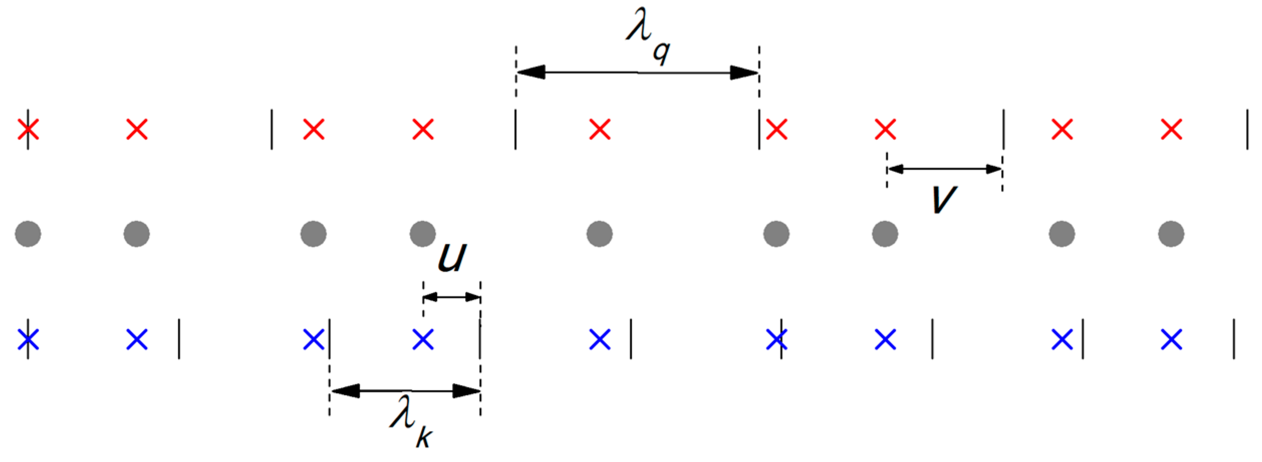
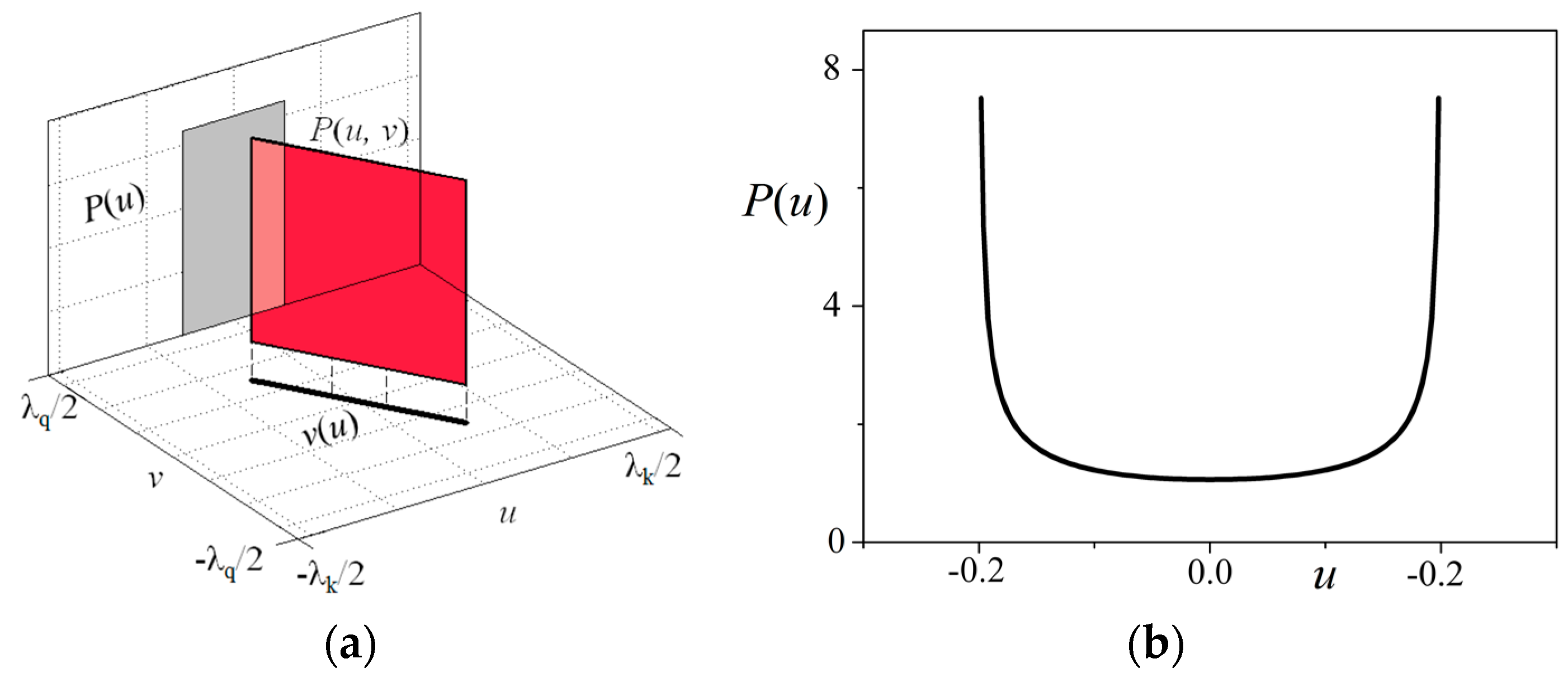
2. The Average Unit Cell (AUC) Concept and the Statistical Method

One of the drawbacks of superspace description is that the atomic surfaces are non-physical objects identified as multidimensional atoms. The statistical method keeps all considerations in the physical space only, i.e. the space where atoms are arranged in the structure. To explain in details what the average unit cell concept is, let us use a simple 1D model structure, which in general can be periodic or aperiodic. The construction of the average unit cell is illustrated in Figure 1. Beside the atomic structure we need also the so-called reference lattice which is periodic with lattice constant ${\lambda }_k$ related to the length of some vector $k_0$ as ${\lambda }_k=\frac{2\pi }{k_0}$. To take full advantage of our description (in terms of structure analysis) vector $k_0$ must be a basic scattering vector in the reciprocal space where the diffraction image is observed. In general there are no restrictions on the choice of reference lattice constant other from ${\lambda }_k$, it is, however, most useful to relate ${\lambda }_k$ with $k_0$. New atomic positions $u$ in the AUC are obtained as projections of original atomic positions onto reference lattice and calculated with respect to the nearest node of a reference lattice. Mathematically it is achieved by modulo operation. Each position $x_j$ of atom j can be defined in the AUC reference frame as:

$$u_j=x_j \text{mod} {\lambda }_k.$$

(1)

Inversely, atomic positions in physical space, $x_j$, can be retrieved from the AUC as:

$$x_j=\alpha {\lambda }_k+u_j,$$

(2)

where $\alpha$, being an integer, numerates consecutive periods in the reference lattice frame. It is easy to notice that values $u_j$ are limited to a region $\langle -\frac{{\lambda }_k}{2},\frac{{\lambda }_k}{2})$ or $\langle 0,{\lambda }_k)$, depending on a definition, and form a distribution. After normalization this distribution gains a statistical meaning. Numerical calculations confirmed by analytical considerations performed for different model structures show the characteristic feature of such distribution—for large enough systems it is well-defined, limited and in many cases dense. The distribution, denoted as $P(u)$, is called the average unit cell. Its shape is characteristic for a given structure type, but also for amount of disorder and size of a structure (coherence length), which is discussed in details in further parts of this paper.

In case of aperiodic systems, like quasicrystals, yet another reference lattice is needed to describe fully aperiodic structure and its diffraction pattern. We introduce a lattice with lattice parameter ${\lambda }_q=\frac{2\pi }{q_0}$, where $q_0$ is another reciprocal-space vector, called modulation vector, and is usually related to $k_0$ by a scaling property, i.e. $q_0=\frac{k_0}{\xi }$ with $\xi$ being a scaling factor. The term “modulation vector” is known in the crystallography of modulated structures and refers to the positions of satellite reflections in the diffraction diagram. Scaling factor is responsible for commensurateness of a modulation—it can be rational or irrational number. In the case of quasicrystals, it is often equal to $\tau \approx 1.618$, which is the golden mean value (so called $\tau$-based quasicrystals for which diffraction peaks’ positions scale with $\tau$). Introducing another reference lattice has the same reasons as introducing doubled dimensionality in superspace description—it is forced by aperiodicity. We define positions $v_j$ of atom j and their distribution function $P(v)$ in an analogous manner as for the reference lattice ${\lambda }_k$ before. Values $v_j$ are restricted to a region $\langle -\frac{{\lambda }_q}{2},\frac{{\lambda }_q}{2})$ (or equivalently: $\langle 0,{\lambda }_q)$). The complete information of a structure is stored in a full distribution function $P(u,v)$, which is the distribution of atomic positions projected onto both reference lattices. The total function $P(u,v)$ is a fundamental definition of an AUC. However, the scaling property of a structure, if present, enforces a characteristic behavior of $P(u,v)$, namely the function is non-zero only along a certain curve $v(u)$ in parameter space $(u,v)$, which is strongly dependent on scaling factor $\xi$. It is worth noting that the distribution $P(u,v)$ is not a 2D function, since coordinates $u$ and $v$ are defined along one direction in space—they do not span a 2D space. The distribution $P(u,v)$ must be instead considered a 2-parameter distribution function. If the scaling property is known, the marginal distributions—$P(u)$ or $P(v)$—store the full structural information of a system. Mathematically, it can be obtained from $P(u,v)$ by integration over one parameter, e.g., $P(u)={\int }_0^{{\lambda }_q}P(u,v)\mathrm{d}v$. We usually consider $P(u)$ as the AUC. In Figure 2a the marginal distribution with respect to a full distribution is shown in the case of 1D quasicrystal modeled by a Fibonacci chain. The distribution $P(u)$ is a most fundamental object in the statistical approach, which enables calculating the full diffraction patterns, but also considering structural disorder or sample finite size effects. The situation changes if the structure becomes not ideal, e.g., exhibits atomic disorder. Then, the scaling relation $v(u)$ can be violated and the full distribution $P(u,v)$ must be considered.

The simple interpretation of a distribution $P(u)$ applies for vertices of a “lattice” in aperiodic crystals (it is quasilattice in case of quasicrystals or underlying periodic lattice in case of incommensurately modulated structures). The atomic decoration of the “lattice” in positions other from vertices naturally subdivides the AUC. The same feature is observed in modeling of atomics surfaces in superspace description. It is of course possible to find a shape of AUC for decorated model structure, but from practical point of view—rather unnecessary. In a refinement process the decoration is to be refined or found in general. It is more efficient to include an atomic decoration in a structure factor independently from “lattice” part, the information of which is kept in the $P(u)$ shape.

2.1. AUC for Periodic Structures

The basic scattering vector of a periodic lattice with lattice parameter $a$ is $\frac{2\pi }{a}$. The reference lattice constant ${\lambda }_k$ is equal to a, which implies that the distribution $P(u)$ is simply a Dirac delta function centered at $u=0$. Of course, by choosing $\lambda \ne a$, but commensurate, the distribution will be fragmented but still built of Dirac deltas distributed over entire region $\langle 0,\lambda )$ in positions dependent on $\lambda /a$ ratio with heights restricted by normalization condition of $P(u)$. The shape of $P(u)$ has no internal structure and reduces simply to a crystallographic unit cell known for periodic crystals.

2.2. AUC for Quasicrystals

The statistical method was first applied to 1D model quasicrystal—Fibonacci chain in [16]. The Fibonacci chain can be constructed with a sequence of long $L$ and short $S$ distances whose length ratio tends to $\tau$ in infinite system. Golden mean is a scaling factor in most types of known quasicrystals. Segments $L$ and $S$ follow a recurrence rule $L\to LS, S\to L$ after each iteration step. Such sequence is fully aperiodic but perfectly deterministic and ordered [4,10,17]. Endpoints of the segments define nodes of the “lattice” which becomes a quasilattice of 1D quasicrystal. The full distribution $P(u,v)$ and marginal distribution $P(u)$ as well as scaling relation $v(u)$ for a Fibonacci chain are presented in Figure 2a. $P(u,v)$ is dense and uniform and non-zero only along segment line $v=-{\tau }^{2}u$ which is called TAU2-scaling [18]. In fact, the TAU2-scaling can have a constant shift $b$ which expresses non-centrosymmetricity of $P(u,v)$, for details see [19]. The width of $P(u)$ is dependent on a chosen vector $k_0$. For a Fibonacci chain an average interstitial distance is known to be ${\lambda }_k=\frac{{\tau }^2+1}{\tau +1}\approx 1.38$ (a.u.). The basic scattering vector is in this case $k_0=\frac{2\pi {\tau }^2}{{\tau }^2+1}\approx 4.54$ (a.u.). This scattering vector corresponds to a (1,1)-peak position in 2D reciprocal space in the superspace approach. For such a choice of $k_0$ a width of distribution $P(u)$ is $u_0=\frac{1}{\tau }$ and its height $P_0=\frac{1}{u_0}=\tau$. If different scaling property is chosen, the characteristic parameters $k_0,{\lambda }_k,u_0$ are expressed by $\xi$ instead of $\tau$.

1D quasicrystal is just a model example but does not restrict a generality of the statistical approach to modeling of real quasicrystals. More realistic model quasilattices are built by Penrose tiling (model of 2D decagonal quasicrystal) and Ammann tiling (model of 3D icosahedral quasicrystal). TAU2-scaling applies for both cases. The shapes of AUCs are the following: 4-parameter distribution $P(u_1,u_2,v_1,v_2)$ for Penrose tiling is spanned by 4 two-dimensional pentagons (2 smaller and 2 bigger) [20,21,22]; 6-parameter distribution $P(u_1,u_2,u_3,v_1,v_2,v_3)$ for Ammann tiling takes form of 3D Keplerian solid—rhombic triacontahedron [15,23]. To construct AUCs for 2D and 3D quasicrystals we need to span pairs of reference lattices which are 2D or 3D, respectively. Depending on the choice of basic scattering vectors $k_0$ (orthogonal or oblique vector basis), which are now 2D or 3D, the AUCs undergo different deformations of regular pentagons or triacontahedron [24,25]. Similarly, the width $u_0$ in case of Fibonacci chain depends on the choice of $k_0$.

2.3. AUC for Harmonically Modulated Structure

Let us now consider 1D modulated structure with harmonic displacive modulation given by single sine function. Every atomic position of this structure can be expressed as

$$x_n=na+A \text{sin}(q_{0}na),$$

(3)

with $n$—atomic position with respect to nth unit cell; $a$—unit cell size (parameter of the underlying periodic lattice); $A$—modulation amplitude (usually small value in comparison to $a$); $q_0$—modulation vector (in the reciprocal space). The modulation vector can be either commensurate or incommensurate with respect to basic reciprocal space vector $k_0$, which is related to lattice parameter $a$. By this, we distinguish commensurately and incommensurately modulated structures. Vector $q_0$ can be defined again as $q_0=\frac{k_0}{\xi }$ with scaling factor $\xi$ expressing the commensurateness. The distribution $P(u)$ for harmonically modulated structure is given by far more complex shape than in previous cases. The characteristic U-like shape (see Figure 2b) can be analytically define as

$$P(u)=\frac{1}{\pi A\sqrt{1-{\left(\frac{u}{A}\right)}^2}}.$$

(4)

It diverges at $u=\pm A$, but is normalizable and integrable [26]. The scaling relation $v(u)$ takes a form of modified arcsine-like shape, which is a continuous function well defined in three intervals (see Figure 2c):

$$v(u)=\{\begin{array}{ll}\frac{1}{q_0}{\text{sin}}^{-1}\left(\frac{u}{A}\right)+u,& u\in \langle -A,A\rangle \\ \frac{1}{q_0}\left[-{\text{sin}}^{-1}\left(\frac{u}{A}\right)+\pi \right]+u,& u\in (0,A\rangle \\ \frac{1}{q_0}\left[-{\text{sin}}^{-1}\left(\frac{u}{A}\right)-\pi \right]+u,& u\in \langle -A,0)\end{array}.$$

(5)

Exact analytical derivations require a little mathematics but are necessary in terms of a derivation of the structure factor formula. All calculations are performed in details in [27].

2.4. AUC for Thue-Morse Sequence

A Thue-Morse sequence, defined by binary recurrence rule $a\to ab, b\to ba$ with arbitrary $a$ and $b$ segments, can be used to construct a very special chain-structure which is aperiodic, but not chaotic, with singular-continuous component in the diffraction pattern [4,28,29]. The structure is perfectly ordered but completely aperiodic even in high dimensions. In this case, the statistical description finds its great application [30]. For a construction of AUC we have again some freedom of choosing the reference lattice. Let us choose a reference lattice parameter ${\lambda }_k=a+b$ with center of interval $\left(-\frac{\lambda }{2},\frac{\lambda }{2}\right)$ in a position $a+b$ (see Figure 2d). Basic scattering vector is $k_0=\frac{2\pi }{a+b}$. If we consider large enough number of atoms (formally tending to infinity), occupation probability of center position gets $1/2$ and positions $b$ and $–b$ (position $–b$ corresponds to position $a$) take the probability $1/4$ each. The above holds for the Bragg peaks in the diffraction diagram, which are periodic in case of the Thue-Morse chain. However, also the singular continuous part in the diffraction pattern can be successfully solved within statistical method. The full AUC shape strongly depends on the scaling factor $\xi$, and by this on modulation vector $q_0$, but not only. For completely aperiodic sequences like Thue-Morse chain also the sample size (number of atoms $N$ in the chain) is crucial. Coherence length strongly influences the singular continuous part of a diffraction pattern. This feature must be also considered during construction of AUC. For instance, if the number of atoms in sequence is given by multiples of 6 at scaling factor $\xi =3$, the probability distribution values take 9 non-zero positions of heights proportional to $1/6$. For further details see [15,30]. Summarizing, for the Thue-Morse aperiodic sequence the reference lattice concept allows to designate intensities and scaling properties for the singular continuous part with scattering vector $q_0=k_0/(2m+1)$ with $m$ being integer.

3. Structure Factor Derivation

Structural investigation of materials requires, in most general case, a starting model structure, which is refined against experimental data—usually diffraction data with neutron, X-ray or electron beams. In addition, computational methods, like energetics calculations, are available to refine the structure model. In all cases the starting model is needed and analytical formula for the structure factor must be considered as a function, which allows for simulating the diffraction pattern and comparing it with the measured one. The question is notably important and difficult in the case of complex materials, like aperiodic crystals and particularly quasicrystals, where no periodic unit cell is available. The statistical method is perfectly suitable for deriving analytical formulas of structure factors for all aperiodic crystals.

Analytical derivation of structure factor formula in the statistical approach takes full advantage of Fourier transforming properties. Starting from a definition, the structure factor can be written as

$$F(k)={\sum }_{j=1}^N{f}_j\text{exp}[ik{x}_j],$$

(6)

where $x_j$ is the atomic position in the structure, $k$ is the scattering vector length (in reciprocal space), $f_j$ is a scattering form factor for $j$-th atom, $i$ is an imaginary unit and summation is over all $N$ atoms in the structure. In further parts parameters $f_j$ will be omitted. This, however, does not limit our consideration to monoatomic decorations only (see the comment at the end of the Section 3.1). We can now use our statistical interpretation of atomic positions expressed in reference lattices ${\lambda }_k$ and ${\lambda }_q$ frame (see formula (2)). In addition, an arbitrary scattering vector can be written as $k=n{k}_0+m{q}_0$ with $n,m$ being integer indices. Structure factor now takes the form

$$F(k)=F(n,m)={\sum }_{j=1}^N\text{exp}[in{k}_0(\alpha {\lambda }_k+u_j)+im{q}_0(\beta {\lambda }_q+v_j)]={\sum }_{j=1}^N\text{exp}[in{k}_0{u}_j+im{q}_0{v}_j],$$

(7)

where $\alpha ,\beta ,n,m$ are integers and $u_j,v_j$ are coordinates of atoms in the AUC constructed for reference lattices ${\lambda }_k$ and ${\lambda }_q$ respectively. From discussion in Section 2 we know that values $u_j,v_j$ densely fill the limited space (they form a well-defined distribution $P(u,v)$) and are usually not independent (scaling relation $v(u)$). This entitles us to replace summation in (7) with integration over the AUC shape. Finally, the structure factor $F$ in one-dimensional case for scattering vector $k$ can be expressed by means of a generalized two-mode Fourier transform [16,25,31]:

$$F(k)=F(n,m)={\int }_0^{{\lambda }_k}{\int }_0^{{\lambda }_q}P(u,v) e^{i(n{k}_{0}u+m{q}_{0}v)}\mathrm{d}u\mathrm{d}v,$$

(8)

with further simplification possible due to scaling relation $v(u)$. The use of scaling properties of aperiodic sets in the two-mode Fourier transform (8) effectively reduces the dimensionality of the problem by half. This will be effectively used in the following subsections. We focus on purely “geometric” structure factor with no corrective factors. As mentioned already in Section 2, the “atomic” part of the structure factor can be separated from the “lattice” part. Atomic decoration appears as phase factor to the complete structure factor formula.

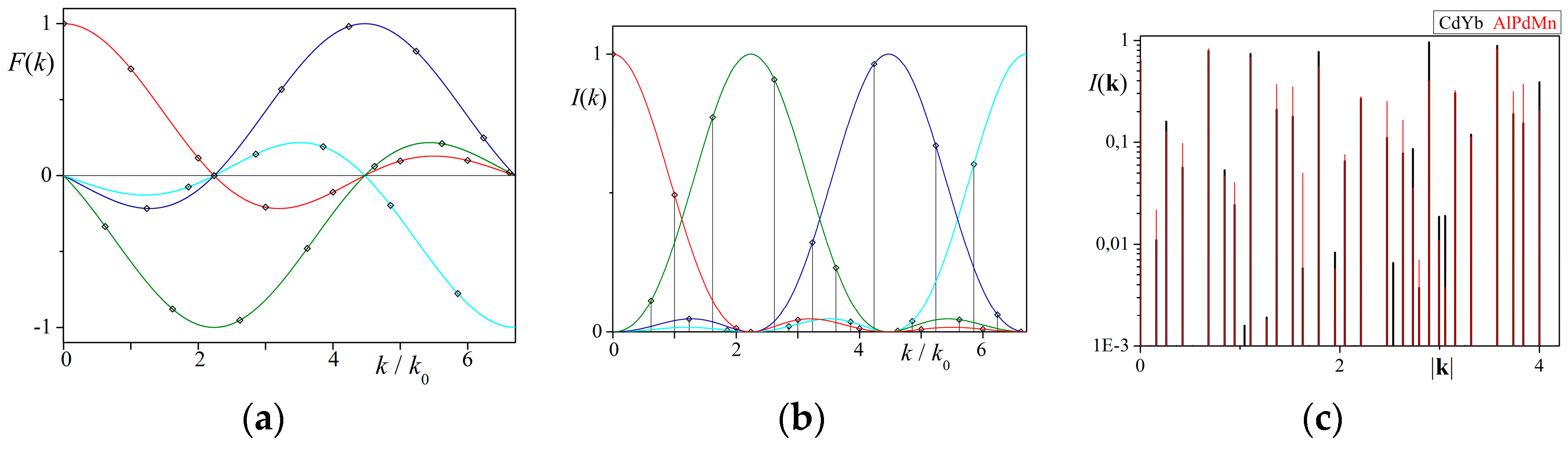
3.1. Structure Factor for Quasicrystals

1D Fibonacci chain is the easiest structure model of a quasicrystal. All conclusions obtained here apply equally to the model decagonal and icosahedral quasicrystals. Scaling factor $\xi =\tau$ leads to characteristic TAU2-scaling relation $v=-{\tau }^{2}u$, which significantly simplifies integration in (8). The structure factor for Fibonacci chain takes the form

$$F(k)=F(n,m)={\int }_0^{u_0}P(u) e^{i{k}_{0}u(n-\tau m)}\mathrm{d}u,$$

(9)

which after simple calculation gives:

$$F(w)=e^{-i\frac{w{u}_0}{2}} \frac{\text{sin}\left(\frac{w{u}_0}{2}\right)}{\left(\frac{w{u}_0}{2}\right)},$$

(10)

where $w=k_0(n-\tau m)$ is reduced scattering vector, $u_0=\frac{1}{\tau }$ is the width of $P(u)$ distribution. The phase factor (exponent in (10)) stands for possible non-centrosymmetricity of $P(u)$, the structure factor formula is in general a complex number. After symmetrizing the distribution one gets the real form which can be expressed again in $k$:

$$F(k)=\text{cos} (m\pi ) \frac{\text{sin}\left((k-m{k}_1)\frac{u_0}{2}\right)}{\left((k-m{k}_1)\frac{u_0}{2}\right)},$$

(11)

where $k$ is the scattering vector length (any continuous value $k$ is possible) and$k_1=k_0\left(\tau +\frac{1}{\tau }\right)=\sqrt{5}{k}_0$ is a shift vector which interpretation will be delivered later. For centrosymmetric distribution $P(u)$, which is always possible to obtain, the phase in structure factor formula is only $0$ or $\pi$ (for even and odd values $m$, respectively). The intensity of a diffraction reflection at any position $k$ can be easily calculated as squared modulus of the structure factor, i.e., $I(k)={|F(k)|}^2$, and for Fibonacci chain it is given by characteristic shape of ${\text{sin}}^2(x)/x^2$ function. The $F(k)$ and $I(k)$ plots for the Fibonacci chain are shown in Figure 3a,b.

Transformation from (9) to (10) gives us an interesting interpretation of a distribution $P(u)$–its Fourier transform (10) defines the so-called envelope function [31]. An envelope connects tops of the diffraction peaks sharing the same value $m$. For all other peaks we observe a shift of an envelope by vector $k_1$ first used in formula (11) (this is the interpretation of $k_1$). The full diffraction pattern of 1D Fibonacci chain, obtained by applying formula (11), is composed of periodic series of peaks with period $k_1$ belonging to a common envelope function and peaks distributed within envelopes with period $k_0$. These characteristics holds true not only for quasicrystals, but also for commensurately and incommensurately modulated crystals, as well as periodic crystals. Formula (9) can be rewritten to a more general form which makes use of periodically expanded AUC (denoted as $P_{\text{exp}}(u)$), what leads to a universal tool applicable for diffraction analysis of any structure type. A Fourier transform of such periodic structure calculated using the following equation:

$$F(k)={\displaystyle \sum _m}{e}^{-im\theta }{\displaystyle \underset{-\infty }{\overset{\infty }{\int }}}{P}_{\text{exp}}(u)e^{-i(k-m{k}_1)u}\mathrm{d}u$$

(12)

leads to a complete diffraction pattern of all $(n,m)$-peaks, whereas conventional Fourier transform (9) gives the envelope function. What is important to note is that all reflections belonging to a common envelope function have identical phase (denoted as $\theta$). The phase changes whenever an envelope passes through zero (see equation (11)). Such behavior enables calculating phases of a structure factor directly from a diffraction pattern with no need of using iterative phase-retrieval algorithms. Having complete diffraction pattern one can reduce it to reduced scattering $w$ and by inverse Fourier transform obtain a probability distribution $P(u)$ and, eventually, the full information of the structure. For details see [32]. Formula (12) can be applied to numerous structure types with different scaling factors exhibiting quasicrystalline diffraction pattern. Such concept, with potential application to structure refinement of complex systems, was proposed in [25] with all details given.

As a confirmation of utility of the statistical method applied to arbitrary decorated structure numerous decagonal quasicrystals modeled by the (rhombic) Penrose tiling were successfully refined in [33,34,35]. In addition, for an icosahedral quasicrystal modeled by the Ammann tiling the structure factor for arbitrary decoration and the so-called simple decoration scheme was derived and discussed in [23,36]. The latter structure factor takes the form [23]:

$$F(\mathit{k})={\sum }_{o=1}^{10}(F{(\mathit{k})}_o^{AR}{\sum }_{j=1}^{N_{AR}}{f}_j{\alpha }_j{e}^{i\mathit{k}·{\mathit{r}}_{\mathit{j}}})+{\sum }_{o=1}^{10}(F{(\mathit{k})}_o^{OR}{\sum }_{j=1}^{N_{OR}}{f}_j{\alpha }_j{e}^{i\mathit{k}·{\mathit{r}}_{\mathit{j}}}),$$

(13)

with $F{(\mathbf{k})}_o^{\text{AR}}$/$F{(\mathbf{k})}_o^{\text{OR}}$ being Fourier transforms of parts of the AUC corresponding to a given orientation $o$ of the rhombohedra. Ammann tiling is built of two prototiles-acute (AR) and obtuse (OR) rhombohedra, which volume ratio remains $\tau$ and faces are spanned by golden rhombuses [10,37]. It is a known fact that 3D aperiodic quasilattice can be spanned by the two types of rhombohedra taking each 10 symmetrically independent orientations in space. For that reason index $o$ runs over ten different orientations. As mentioned in Section 2.2 the AUC for Ammann tiling has a shape of rhombic triacontahedron. The parts related to 20 orientations of rhombohedra have again rhombohedral shapes. Each prototile can be in general decorated by $N_{\text{AR}}$/$N_{\text{OR}}$ atoms. The $j$-th atom is placed at the position ${\mathbf{r}}_j$ with respect to the reference vertex of an rhombohedron and depending on the position gives a fraction ${\alpha }_j$ of one to the total sum. Parameters $f_j$ are atomic form factors of each atom $j$. Atomic decoration is the phase factor to the complete structure factor formula, as already mentioned. The formula (13) was recently confirmed for simple decoration scheme, where atoms are placed in the vertices and mid-edges of the rhombohedra. An acute rhombohedron has additional 2 atoms on the long body-diagonal. Such a decoration scheme allows for considering binary and ternary icosahedral systems. The diffraction pattern of exemplary Cd-Yb and Al-Pd-Mn decorations was presented in Figure 3c. This picture shows how useful the structure factor formula derived within statistical description can be in terms of arbitrary decorated quasicrystalline structure based on model tilings. For all details see [36].

3.2. Structure Factor for Modulated Structures

A statistical approach was applied to modulated structure initially in [26,38], but comprehensive considerations were performed in [27]. As discussed in Section 2.3 calculations within statistical method require slightly more advanced mathematics. The method allows, however, for fully analytical derivation of the structure factor formula with no need of complex expansion methods used in classical approach to the subject [39,40,41]. General formula (8) can be again reduced to 1D integration over distribution $P(u)$ given in (4) in 3 intervals defined in (5). As shown in details in [27] the result of integration is a known fact that the structure factor for harmonically modulated structure with single modulation component is given by Bessel function of the first kind:

$$F(k)=J_{-m}\left(k_{0}A\left(n+\frac{m}{\xi }\right)\right)=J_{-m}(kA),$$

(14)

where $k=k_0\left(n+\frac{m}{\xi }\right)$ and $\xi$ being the scaling factor defining a commensurateness of a modulation. Notation from Section 2.3 was used. Integer indices $n$ and $m$ numerate main and satellite reflections respectively. The diffraction pattern is again composed of series of peaks grouped to envelopes defined by Bessel functions of the consecutive order $–m$ (see Figure 4). The series are this time not periodic, as the zeros of Bessel function are not periodic. Using statistical description we also showed a close similarity between quasicrystals and incommensurately modulated crystals. It appears that 1D quasicrystal, modeled by the Fibonacci chain, can be understood as a modulated structure with multiple modulation vectors being the higher order Fourier expansion of the basic modulation term [27,38].

3.3. Structure Factor for Thue-Morse Sequence

The structure factor corresponding to Bragg component of a diffraction pattern can be easily found as a sum of atomic occupation terms weighted with occupation probabilities $P_i$ of each site (in Figure 2d $P_0=\frac{1}{2}, P_a=P_b=\frac{1}{4}$). This gives a formula:

$$F(k_0)=\frac{N}{2}(1+\text{cos}(k_{0}b)),$$

(15)

Peak intensities scale with number of atoms as $N^2$ what is characteristic for Bragg reflections. The singular continuous part of the diffraction pattern scales fractally with $N$ and is still possible to be described by statistical method. The calculations are difficult and different for different class of number of elements in the chain. Details can be found in refs. [15,30]. The complete diffraction pattern of Thue-Morse chain is presented in Figure 4c.

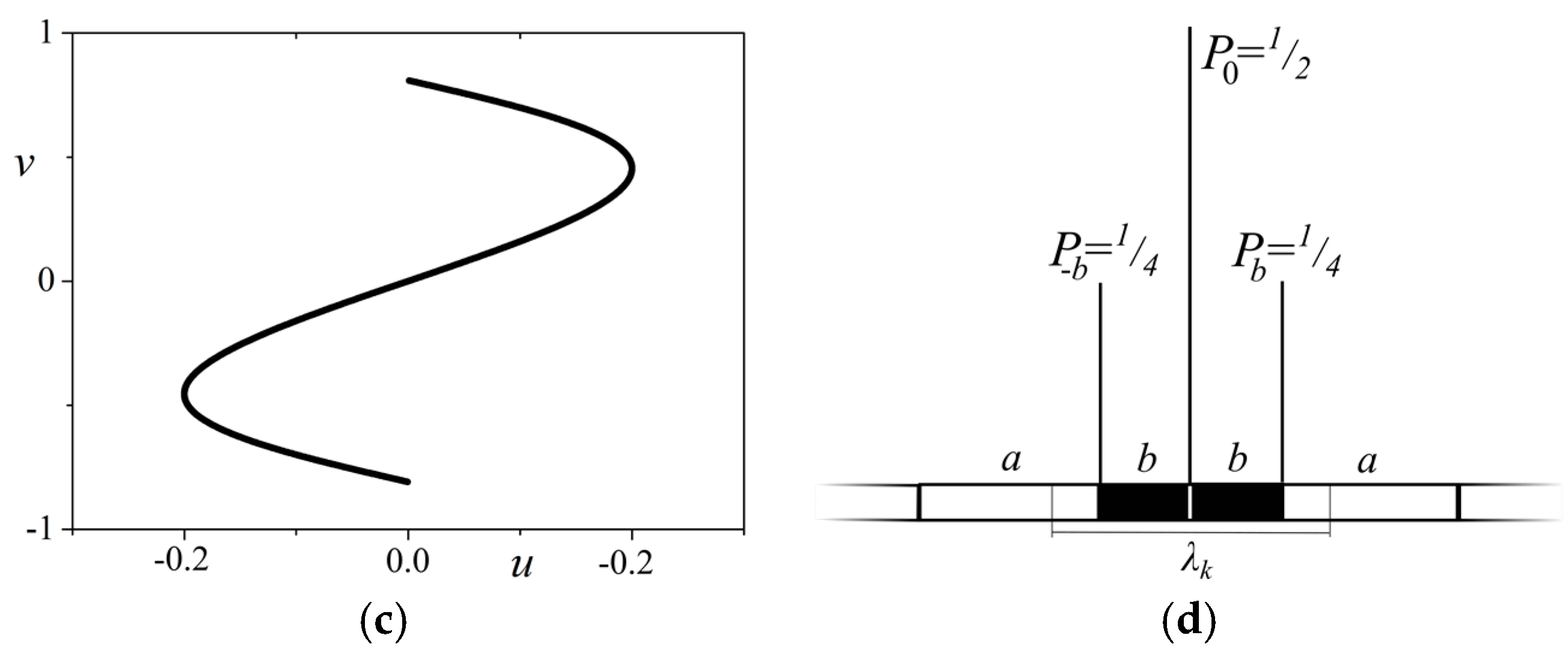
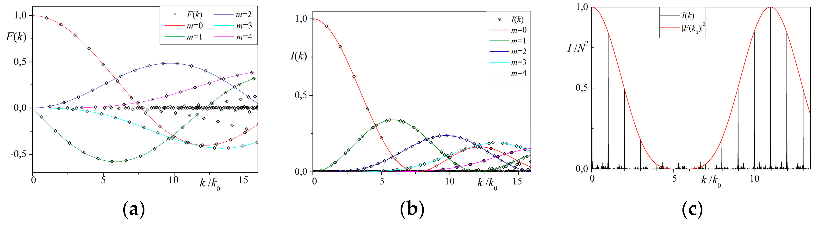
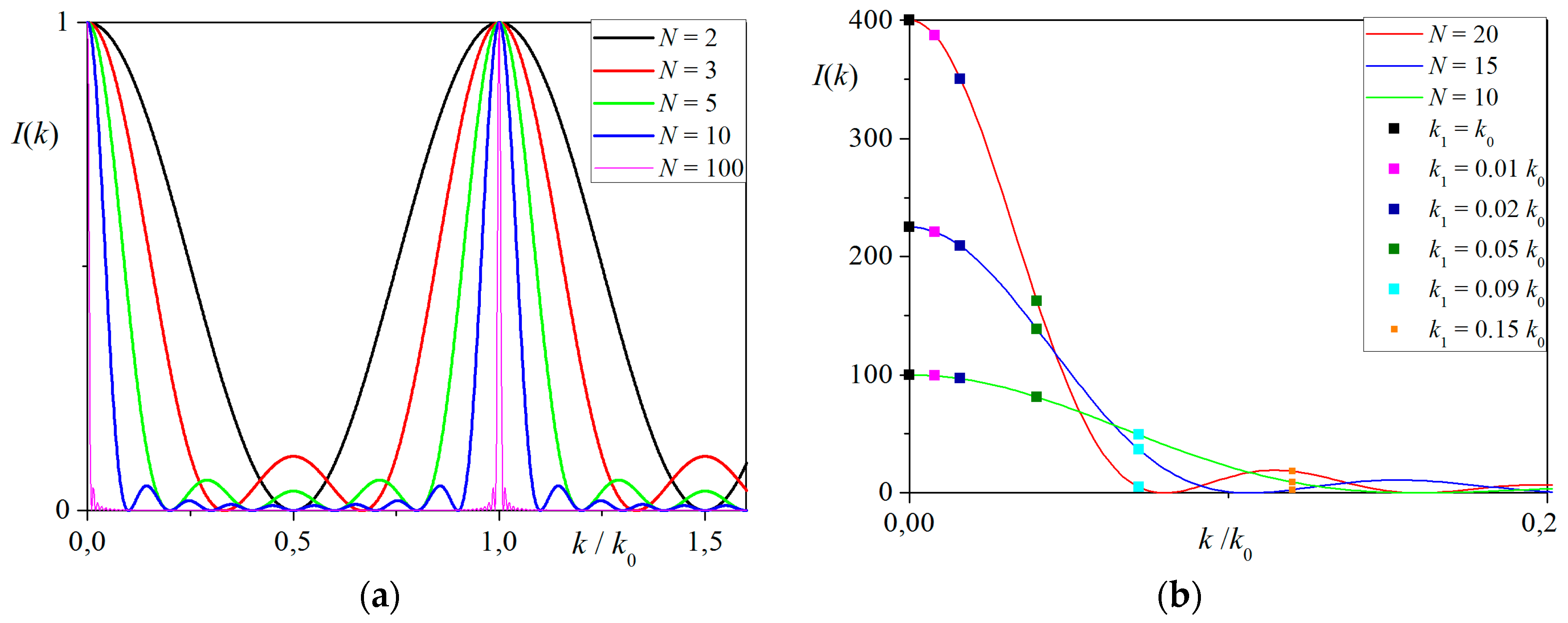
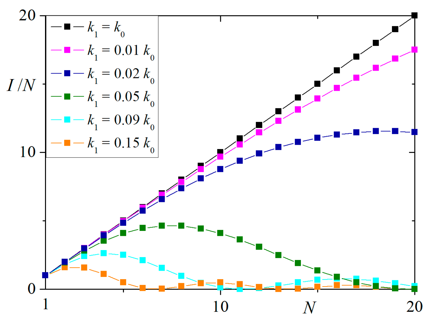
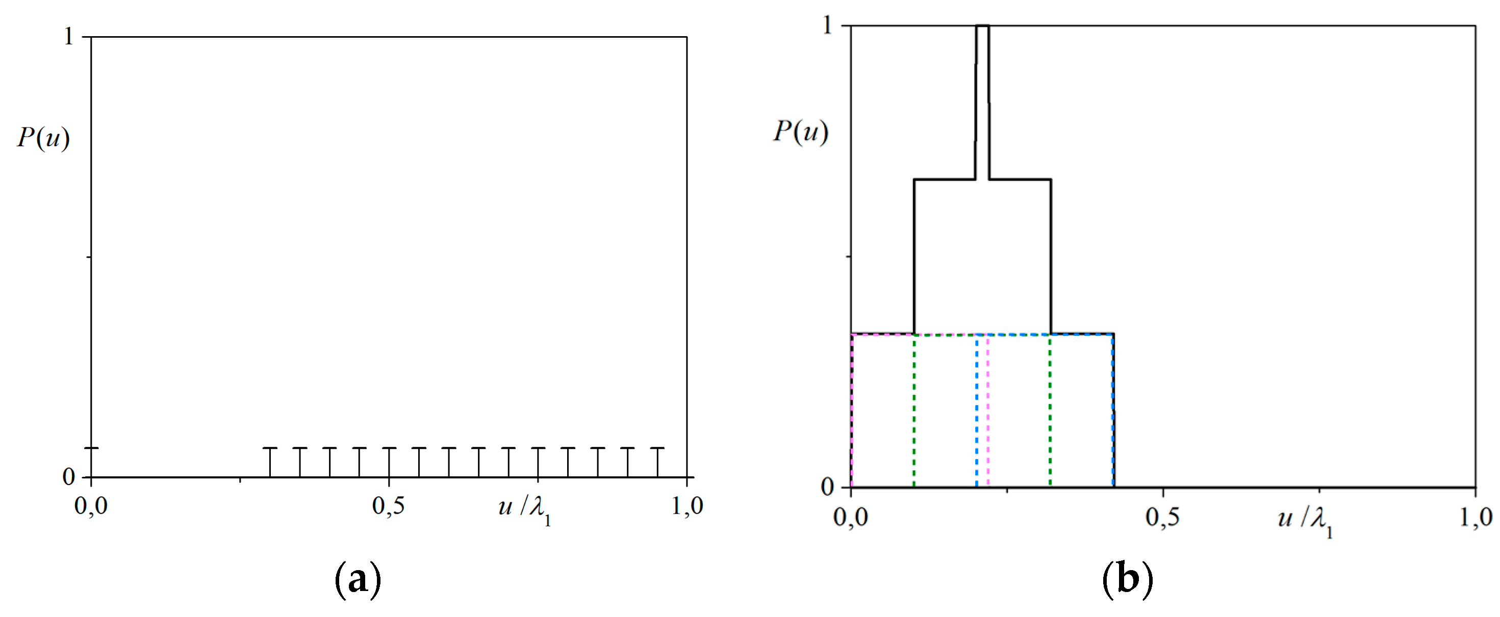
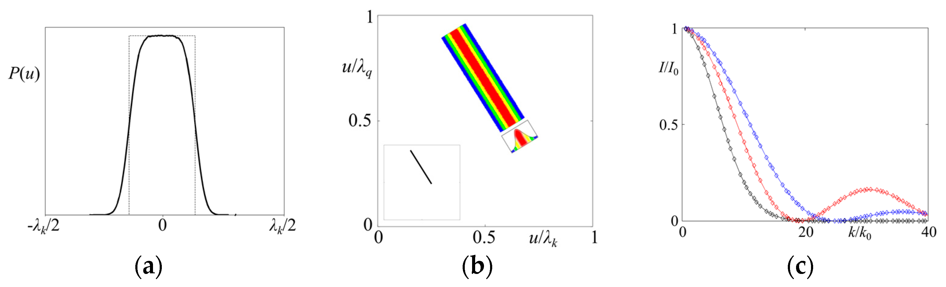
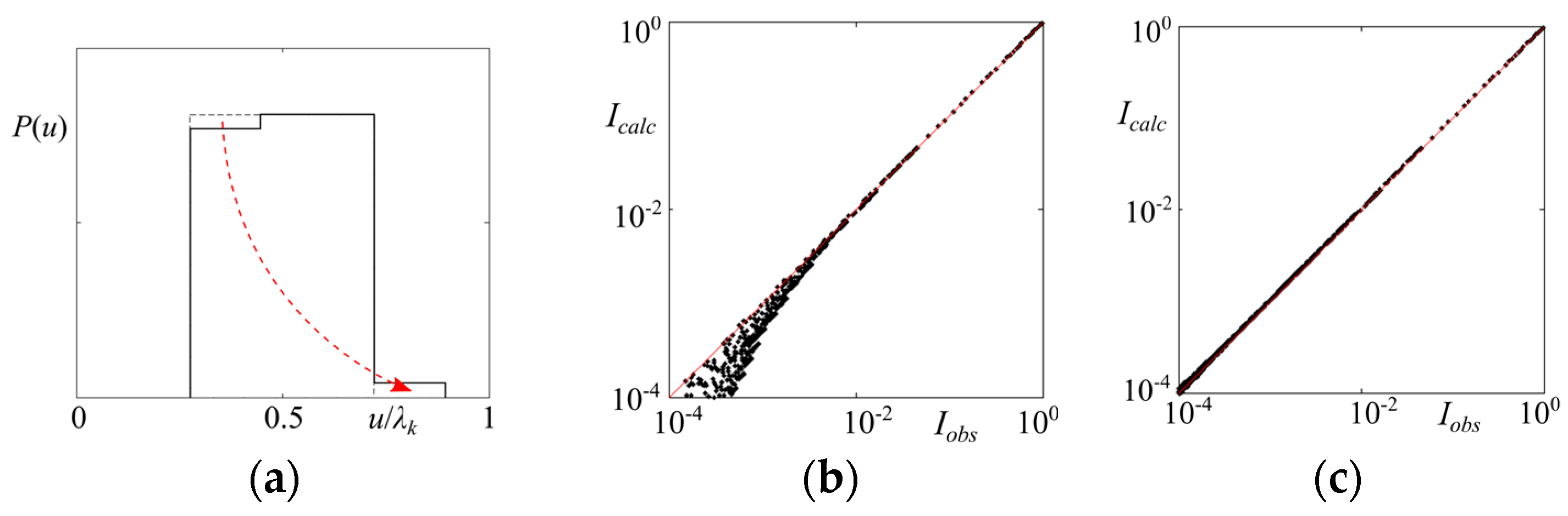
4. AUC-Based Analysis of a Peak Profile

This section shows how the statistical method can be involved to analyze the profile of a diffraction peak. Despite more than 100 years of modern crystallography the theory of diffraction is still being developed and new phenomena are revealed. One of the important topics is the peak profile, which may contain important information on the sample, like size of the crystallites or spatial coherence length of the crystalline material. The known Scherrer formula relates the size of a crystallite with line broadening and is still being developed in terms of nano-crystalline materials and better accuracy of determining the crystallite size [42]. In addition, spatial coherence of the impacting X-ray beam is being studied in terms of peak broadening [43], however the very interesting influence on the peak profile has the coherence length understood as number of scatterers (atoms) in the crystal structure. It has been shown within kinematic theory of scattering that the peak broadening decreases with number of atoms in the chain but only for crystallites smaller than the X-ray spatial coherence length [44]. In another case, the peak width is crystallite-size-independent. Recently, the structure refinements with no analytical functions for profile fitting are tested for powder samples [45]. Proper handling with the peak profile is admittedly an important task during the structure refinement process.

In our studies we performed a simulated diffraction experiment on the periodic chain of point-like scatterers (analogously to the multiple slit diffraction experiment). Numerical Fourier transforming of atomic chain was performed as a simulation of real experiment—the numerically obtained data can be treated as “measured” data. Simple calculations show how the diffraction peak profile strongly depends on number of atoms $N$ (see Figure 5). As already mentioned, with increasing number of atoms the line broadening gets smaller tending to Dirac-delta-like peaks. The positions of consecutive peak-maxima are counted by main scattering vector $k_0$, where $k_0=\frac{2\pi }{a}$ with $a$ being the constant lattice parameter of the atomic chain. In the next plot (Figure 6) the plot of intensities $I$ measured for different scattering vectors $k_1$ taken from a close vicinity of $k_0$ is presented vs. number of atoms $N$. For clarity the figure shows $I/N \text{vs}. N$ plot. For $k_1=n{k}_0, n\in \mathbb{Z}$ the behavior is linear meaning that diffraction intensities measured at centers of broadened peaks are proportional to number of atoms squared. This is known to be a Bragg spectrum of a diffraction pattern ($I\propto N^2$). The successive deviation from a straight line in the Figure 6 is observed for intensities measured at $k_1$ slightly differing from $k_0$ (e.g., $k_1=(1.01-1.15) k_0$ as shown in the figure). Diversity of the scaling $I(N)$ opens a possibility of various interpretations of a peak profile. Using the statistical approach it is possible to construct the distribution $P(u)$ for different $k_1$-s and model the diffraction pattern for a comparison with measured one. Positions $u$ in the AUC can be now calculated modulo ${\lambda }_1=\frac{2\pi }{k_1}$. The exemplary distributions $P(u)$ are shown in the Figure 7. For the record, the AUC constructed for main scattering vector $k_0$ in the case of periodic structure takes a form of a single Dirac-delta peak at $u=0$. The same distribution obtained for $k_1\ne k_0$ gets fragmented and reduced. Its shape depends on the sample size (parameterized by number of atoms $N$). If the periodic chain is replaced by an aperiodic one, like the Fibonacci chain, the distribution $P(u)$ gains an internal structure (with given width and height). If it is constructed for the scattering vector $k_1$ rather than $k_0$ it can take the form presented in the Figure 7b. Summarizing, it is possible to use the statistical method to construct AUCs for different scattering vectors included in the peak profile and model the diffraction pattern of a finite-size sample. Such modeling is also possible in a reversed way – given the diffraction pattern with broad peaks the shape of distribution $P(u)$ is possible to obtain and coherence length (number of atoms $N$ in the scattering crystal volume) can be retrieved.

5. Structure Disorder in Aperiodic Crystals

Recent development of the statistical approach to structural description of quasicrystals provided a novel method of proper dealing with disorder observed in real structures. Two challenges of modern crystallography of quasicrystals are: (i) including all weak reflections available from diffraction experiments with use of synchrotron radiation, and (ii) how to explain and “repair” the characteristic bias observed in log-log plots of calculated vs. measured diffraction intensities during the structure refinement procedure. The course is significantly deviating from a straight line in weak reflections regime ($I<{10}^{-2}$ with respect to the strongest reflection), as observed in many refinement results. Modern instruments allow us to collect diffraction datasets of 6 or more orders of magnitude of peak intensities. It is a big challenge to properly process the measured data. One of many corrections during structure refinement process is the Debye-Waller factor correction. It compensates for the perturbations arising from thermal vibrations (phononic term) or flips (phasonic term) of atoms. The Debye-Waller factor can be also generalized to a statistical interpretation [46,47]. The general formula for Debye-Waller factor is $\text{exp}[-k^2{\sigma }^2]$, where $k$ is the scattering vector and $\sigma$ is a variance of the distribution of atomic arrangement (both in physical or perpendicular space). Small peaks, which usually have large perpendicular-space component of the scattering vector in superspace description (see e.g., [35] and supplemental materials), are biased in the modern refinement results. We attributed the latter to the improper corrective factor for phasons, which is standard (exponential) Debye-Waller factor, commonly used in structure refinements of quasicrystals, and proposed a novel method of analysis of phononic and even more phasonic effects within statistical method. For that we performed credible proofs upon model systems (vertex decoration models) based on Fibonacci chain, Penrose tiling and Ammann tiling. In this review, paper we focus on the Fibonacci chain. All “measured” or “observed” data are meant to be numerically obtained by simulated diffraction experiment.

The AUC is highly sensitive to any type of atomic disorder introduced to the structure. Phonons smear a TAU2-scaling along [1,1]-direction in $(u,v)$-space, whereas phasons lead to the fragmentation of marginal distribution $P(u)$. Both effects are easily noticeable. Knowing the fragmentation of $P(u)$ we are able to introduce a phasonic corrective factor at the level of structure factor definition (it is not a multiplicative but an additive factor) with one parameter to fit, which is a number of flips in the structure [48].

5.1. Phonons

The smearing of ideal atomic positions caused by thermal vibrations of atoms around equilibrium can be, in general, modeled by various functions. The most obvious one is the Gaussian function, which has a deep statistical interpretation. However, also other function types, like harmonic or flat, can be equally good. In [49] it was shown that the three listed function types used as generating functions of phonon disorder in model structures (including periodic ones) are reflected in change of $P(u)$ distribution function. As already mentioned, the distribution is an object constructed in physical space, that is why easily maps all the changes of atomic arrangement, like structural disorder. Gaussian smearing of atomic arrangement is simply reflected by Gaussian smearing of $P(u)$ along the [1,1]-direction for $u,v$ coordinates (see Figure 8a). The thing is, however, more complicated, because also $P(v)$ distribution gets changed under phonons. In general, the total $P(u,v)$ distribution is broadened due to phonons. The scaling relation $v(u)$ provides the best tool for considering phononic smearing of the probability distribution. We need the full $P(u,v)$ distribution, depicted in Figure 8b, to properly describe the diffraction pattern. Gaussian smearing of each atomic position leads to smearing of the characteristic TAU2-scaling. After Fourier transforming of a modified $P(u,v)$ it appears that the structure factor formula consists of two factors: one is the structure factor of an ideal atomic structure and the second, multiplicative factor is the Fourier transform of the phonons-generating function. The final formula for the structure factor for system with phononic disorder in case of 1D quasicrystal is following:

$$F(k)=F(n,m)={\int }_0^{{\lambda }_k}{\int }_0^{{\lambda }_q}P(u,v)e^{i(n{k}_{0}u+m{q}_{0}v)}\mathrm{d}u\mathrm{d}v {\int }_0^{{\lambda }_k}G(u_p)e^{i\left(n{k}_0{u}_p+m{q}_0{u}_p\right)}\mathrm{d}{u}_p,$$

(16)

where $G(u_p)$ is the phonons-generating function and $u_p$ is the atomic displacement from equilibrium position reduced to the AUC frame. In the case of Gaussian-type function, the multiplicative factor (integral on the right) is nothing but the Debye-Waller factor known in crystallography as major corrective factor in structure refinement process. Harmonic or flat function $G(u_p)$ leads to Bessel- or cardinal sine-function type of the corrective factor as a direct result of Fourier transforming. For details on the exact mathematical derivation see [49].

Phononic disorder influences strongly intensities of reflections in the diffraction pattern. Figure 8c shows how the intensities calculated for ideal Fibonacci chain are modified by the phononic correction factor. The main conclusion from that picture is that for wide range of reflections, namely $k<20 k_0$, the type of corrective factor used in the refinement is irrelevant. For Gaussian, Bessel and cardinal sine function the behavior of relative diffraction intensities is essentially the same. Significant deviation appears only at distant reflections ($k>20 k_0$). By trial and error, based on the quality of the obtained fit different distributions $G(u_p)$ of position fluctuation with respect to the ideal structure, the final step of a refinement process can be tested.

5.2. Phasons

Phasons, also called phason modes or phason flips, are phenomena characteristic mostly to quasicrystals. In physical space they manifest with rearrangements (flips) of atoms or whole group of atoms in the structure. In model structures, phasons can be identified with flips of tiles (e.g. rhombuses in the rhombic Penrose tiling or short and long distances in the Fibonacci chain). After such swaps, the perfect quasiperiodic order is violated and the structure becomes disordered. The rearrangement of atoms or tiles is an entropic effect—phasonic disorder increases the entropy of the system. By this means, phasons are very important in terms of stability mechanism of quasicrystals. It is a very hot topic in crystallography of quasicrystals and still not a solved problem—are quasicrystals stabilized by energy or entropy? Recent high temperature diffraction measurements and other structural analysis, also for crystalline approximants, opened a new discussion on the problem with preference of entropic stabilization mechanism [50,51,52,53,54]. The origin of phason modes acquires a better understanding in superspace description. The flips appearing in physical space are generated by distortion of a projection strip or, equivalently, by tilt of a cutting plane in higher-dimensional space. For details see [55,56,57]. The current state-of-art theory of phasons was introduced by Lubensky et al. [58,59] and is a hydrodynamic theory. However, during a structure refinement the phasonic disorder is corrected by using Debye-Waller factor in the same form as known for phonons with substituting the physical-space component of the scattering vector with the perpendicular-space component in superspace approach. Phasons are, in effect, corrected by multiplicative exponential term in the structure factor formula. The theory of phasons is still inconsistent and new approach is highly expected. Moreover, we attribute the bias in the fitted vs. measured diffraction data, particularly seen for small intensities, with exponential decay introduced by phasonic Debye-Waller factor. For more details in that subject see [48].

The statistical method delivers an alternative to the analysis of phasons in quasicrystals. The probability distribution $P(u)$ appears to be highly sensitive also to phasonic disorder, as seen in the Figure 9a. The figure presents the AUC of the Fibonacci chain with phason flips introduced by rearrangement of tile-sequence: $LS\to SL$ with a probability $\alpha =5\%$ (called a flip ratio). Parameter $\alpha =5\%$ means that every 20th sequence $LS$ in the chain is being replaced by a sequence $SL$. After such flips the distribution $P(u)$ becomes fragmented with new part appearing in the place where there was no probability density before and its area proportional to $\alpha$. The fragmented AUC can be now Fourier transformed to a structure factor formula. After analytical derivation the phasonic correction function appears to be an additive factor in the following form

$$D_{\text{phas}}(k)={\sum }_{i=1,3}{A}_i\text{sinc}[(k-m{k}_1)d_i],$$

(17)

where summation runs over three subregions of $P(u)$ as depicted in the Figure 9a, $A_i$ and $d_i$ are heights and widths of each region. Cardinal sine function, $\text{sinc}(x)$, can be equivalently replaced by spherical Bessel function of the first kind with order 0, $j_0(x)$. Parameters $m$ and $k_1$ are used in the same sense as in previous sections. Parameters $d_i$ are directly related to the type of flip ($LS\to SL$ or inversely) and are constant for different flip ratios. Therefore, the flip ratio can be straightforwardly obtained from parameters $A_i$, for any given type of flips. For detailed calculations see [49].

In Figure 9b,c the log-log plots of calculated vs. measured intensities are shown for two types of correcting factor used in the refinement. First is the standard phasonic Debye-Waller factor

$$D_{D-W}\left(k_{\text{perp}}\right)=\text{exp}\left[-\frac{1}{16{\pi }^2}{(k_{\text{perp}})}^2{b}_{\text{phas}}\right]$$

(18)

with single fitting parameter $b_{\text{phas}}$, being proportional to the squared atomic displacement in the perpendicular space, and where $k_{\text{perp}}$ denotes a perpendicular-space component of a scattering vector $k$. Second is the factor defined by formula (17). In both cases, the Fibonacci chain with vertex decoration is used as model 1D quasicrystal. It is clearly seen that using a standard $D_{\mathrm{D}-\mathrm{W}}$ correction yields a systematic deviation in the weak reflections part of the plot, as already mentioned. This is because exponential term favors large-$k_{\text{perp}}$ reflections, which are attributed to small intensities in the diffraction diagram (it is a known characteristics of diffraction patterns of quasicrystals), whereas strong reflections (small-$k_{\text{perp}}$) are corrected only slightly. It must be emphasized that for aperiodic structures, particularly for quasicrystals, the amount of weak reflections is much bigger than that of strong ones. The possibility to effectively use weak reflections in the refinement process is therefore of a great importance. Using a statistical approach to the phasonic Debye-Waller correction enables a practical use of weak reflections, whereas the standard “superspace” Debye-Waller factor not.

6. Statistical Approach and Superspace Method

The basic concept behind superspace (higher-dimensional, nD) method is to restore periodicity in high dimensions. The concept was first introduced for modulated crystals with incommensurate modulation [60]. An aperiodic structure becomes periodic when lifted up to high dimensions with atoms replaced by multidimensional atomic surfaces (also called occupation or acceptance domains). Atomic surfaces decorate the nodes of nD structure (usually even/odd vertices, body centers and mid-edges of the nD cubic unit cell). The aperiodic structure is obtained by projecting the higher dimensional structure cut from inside the so-called projection strip (which can be a multidimensional window spanned in superspace) on the lower-dimensional subspace, called parallel space, which is the physical space. The projection strip (window) is spanned along the so-called perpendicular space, which is orthogonal to the parallel space. Atomic surfaces are also constructed in perpendicular space. This is a fundamental of the cut-and-project method [10]. Other possible approach to superspace analysis of aperiodic crystals is to consider a cut in the nD structure with lower-dimensional physical space. The cutting plane needs to be tilted appropriately to obtain a quasiperiodic ordering [8]. In real refinements of quasicrystals the shape of atomic surfaces become usually far more complicated than those constructed for model tilings (4 pentagons for Penrose tiling and rhombic triacontahedra for Ammann tiling) due to proper handling with atomic decoration of the tiles. The superspace method is sometimes called atomic surface modelling method.

It was proven [15,21] that the AUC can be considered as equivalent to an oblique projection of atomic surface onto physical space along direction defined by $k_{\text{perp}}/k_{\text{par}}$, which is the ratio of perpendicular- to parallel-space component of any scattering vector from reciprocal space. In fact, variables $(u,v)$ can be obtained by an oblique projection of the perpendicular-space components of atomic positions (the atomic surface). This 1:1 correspondence is, however, valid only for ideal structures, like a model Fibonacci chain, Penrose tiling or Ammann tiling with no atomic perturbations. The problem occurs while including atomic disorder to the structure. Atomic surfaces remain unchanged, whereas the probability distributions (AUCs) are highly sensitive to any type of disorder, as discussed in Section 5.

As an alternative to the superspace method the statistical method is, however, more general. It can be successfully used for description of not only periodic crystals or quasicrystals, but also modulated structures as well as aperiodic structures with singular continuous components in the diffraction pattern. The latter case would require an infinite-dimensional superspace to properly reproduce all fractal reflections in a diffraction as lifted to high dimensions. Even model aperiodic structures like those generated by Thue-Morse or Rudin-Shapiro sequences as well as amorphous systems are not possible for being considered in superspace description, whereas the statistical method deals perfectly with them [30,61]. Only the physical-space approaches, such as statistical method, allow us to assess the relationship between the peak intensities and the number of atoms involved in the diffraction experiment, what is a key of understanding the singular continuous component of a diffraction pattern. Concluding, probability distributions of atomic positions in the AUC frame (in physical space) can be easily obtained by an oblique projection of the atomic surfaces from high dimensions, whereas the physical-space description cannot be straightforwardly lifted to higher-dimensional one in the most general case.

As already mentioned, the superspace method is simple in mathematical sense, but causes important limitations in terms of physical interpretation of the atomic surfaces. The statistical description gives a unique interpretation of the atomic surfaces. Fourier transform of the envelopes of the structure factor (defined by squared modulus of the formula (10), see Section 3.1) placed in the vertices of multidimensional superspace and spanned along perpendicular space becomes atomic surfaces. Mathematical details as well as interesting conclusions on characteristic features of diffraction patterns of quasicrystals obtained by statistical interpretation of superspace analysis can be found in [19].

7. Summary

The statistical method is a complete theory suitable for structure determination of periodic and aperiodic systems. Any kind of structure can be expressed in terms of the statistical distribution of atomic positions with respect to the periodic reference lattice with lattice constant related to characteristic length-scale present in the structure. As far as periodic crystals are concerned the description of the structure with the use of statistical approach does not differ from the methodology provided by classical crystallography. The average unit cell, defined as probability distribution, is constructed for periodic crystal is the same as unit cell. The full advantage of the statistical description can be exploited when quasiperiodic system is considered. The distribution contains full structural information and it was shown that the structure factor is the Fourier transform of the distribution. The distribution can be constructed for arbitrarily decorated structure but due to calculational reasons and transparency of obtained results the distribution is limited to nodes of quasilattice (for instance, aperiodic tiling). Whole distribution, being sum of distributions for each independent atom would be just too complex for analysis and would not carry any new information.

The shape of the distribution depends on the type of investigated structure. Quasicrystals possess a uniform distribution, whereas e.g. harmonic displacive modulation results with U-like shape. The distribution can be constructed even for structures aperiodic in higher-dimensional space, like Thue-Morse sequence, for which projection scheme reserved for superspace description is not applicable.

The problem of incorporating disorder in the form of phonons and phasons into structural analysis can also be solved within statistical approach because of the immediate occurrence of the latter on the shape of distribution. Although phononic contribution can be carried out traditionally by Debye-Waller factor even for quasiperiodic structures its generalization for phasons, based on higher-dimensional approach, seems to fail in weak-reflections-regime. Phason flips are observable as cuts in the statistical distribution. If those cuts are considered in the structure factor calculations a proper handling of weak reflections in diffraction pattern is possible. Even more, an exact number of flips is possible to estimate due to dependence of the depth of the cut on the probability of phason flip (flip ratio). Therefore, a well-known problem of deviation in the correlation plot of calculated intensities vs. observed ones, attributed by us to improper handling of phasons, can be resolved.

The reference lattice concept can also serve as a tool of probing the peak profile to estimate the coherence length and the size of crystalline domain. The shape of AUC, obtained for scattering vectors in the vicinity of Bragg peaks, depends on the number of atoms’ contribution to scattering process, therefore a coherence length can be obtained.

Although there is equivalency between higher-dimensional and statistical approach in terms of quasiperiodic structures, meaning the AUC can be considered as oblique projection of the atomic surface, the relation is true for defect-free structure solely. The disorder influences changes in the probability distribution, which can be interpreted in statistical meaning but cannot be equally analyzed in higher-dimensional space. Moreover, the statistical approach is generalizable for other types of structures even without counterpart in the higher-dimensional space.

References

1. Shechtman, D.S.; Blech, I.; Gratias, D.; Cahn, J.W. Metallic Phase with Long-Range Orientational Order and No Translational Symmetry. Phys Rev. Lett. 1984, 53, 1951–1954. [Google Scholar] [CrossRef]
2. Levine, D.; Steinhardt, P.J. Quasicrystals: A New Class of Ordered Structures. Phys. Rev. Lett. 1984, 53, 2477–2480. [Google Scholar] [CrossRef]
3. Baake, M.; Grimm, U. Mathematical diffraction of aperiodic structures. Chem. Soc. Rev. 2012, 41, 6821–6843. [Google Scholar] [CrossRef] [PubMed]
4. Baake, M.; Grimm, U. Aperiodic Order; Cambridge University Press: Cambridge, UK, 2013. [Google Scholar]
5. Kalugin, P.A.; Kitaev, A.Y.; Levitov, L.S. 6-dimensional properties of Al(86)Mn(14) alloy. J. Phys. Lett. 1985, 46, L601–L607. [Google Scholar] [CrossRef]
6. Duneau, M.; Katz, A. Quasiperiodic patterns. Phys. Rev. Lett. 1985, 54, 2688–2691. [Google Scholar] [CrossRef] [PubMed]
7. Elser, V. The diffraction pattern of projected structures. Acta Cryst. A 1986, 42, 36–43. [Google Scholar] [CrossRef]
8. Yamamoto, A. Crystallography of Quasiperiodic Crystals. Acta Cryst. A 1996, 52, 509–560. [Google Scholar] [CrossRef]
9. Janssen, T.; Chapuis, G.; de Boissieu, M. Aperiodic Crystals: From Modulated Phases to Quasicrystals; Oxford University Press: Oxford, UK, 2007. [Google Scholar]
10. Steurer, W.; Deloudi, S. Crystallography of Quasicrystals; Springer: Berlin, Germany, 2009. [Google Scholar]
11. Takakura, H.; Yamamoto, A.; Tsai, A.-P. The structure of a decagonal Al72Ni20Co8 quasicrystal. Acta Cryst. A 2001, 57, 576–585. [Google Scholar] [CrossRef]
12. Cervellino, A.; Haibach, T.; Steurer, W. Structure solution of the basic decagonal Al-Co-Ni phase by the atomic surfaces modelling method. Acta Cryst. B 2002, 58, 8–33. [Google Scholar] [CrossRef]
13. Takakura, H.; Gomez, C.P.; Yamamoto, A.; de Boissieu, M. Atomic structure of the binary icosahedral Yb-Cd quasicrystal. Nat. Mater. 2007, 6, 58–63. [Google Scholar] [CrossRef]
14. Wolny, J. The reference lattice concept and its application to the analysis of diffraction patterns. Phil. Mag. A 1998, 77, 395–412. [Google Scholar] [CrossRef]
15. Wolny, J.; Kozakowski, B.; Kuczera, P.; Strzalka, R.; Wnek, A. Real Space Structure Factor for Different Quasicrystals. Isr. J. Chem. 2011, 51, 1275–1291. [Google Scholar] [CrossRef]
16. Wolny, J. Average Unit Cell of the Fibonacci Chain. Acta Cryst. A 1998, 54, 1014–1018. [Google Scholar] [CrossRef]
17. Senechal, M. Quasicrystals and Geometry; Cambridge University Press: Cambridge, UK, 1995. [Google Scholar]
18. Wolny, J.; Kozakowski, B.; Kuczera, P.; Pytlik, L.; Strzalka, R. Real Space Structure Factor and Scaling for Quasicrystals. In Aperiodic Crystals; Schmied, S., Lifshitz, R., Withers, R.L., Eds.; Springer: Berlin, Germany, 2013; pp. 211–218. [Google Scholar]
19. Wolny, J.; Kozakowski, B.; Kuczera, P.; Pytlik, L.; Strzalka, R. What periodicities can be found in diffraction patterns of quasicrystals? Acta Cryst. A 2014, 70, 181–185. [Google Scholar] [CrossRef] [PubMed]
20. Wolny, J.; Kozakowski, B.; Repetowicz, P. Construction of average unit cell for Penrose tiling. J. Alloy. Comp. 2002, 342, 198–202. [Google Scholar] [CrossRef]
21. Kozakowski, B.; Wolny, J. Structure factor for decorated Penrose tiling. Acta Cryst. A 2010, 66, 489–498. [Google Scholar] [CrossRef] [PubMed]
22. Chodyn, M.; Kuczera, P.; Wolny, J. Generalized Penrose tiling as a quasilattice for decagonal quasicrystal structure analysis. Acta Cryst. A 2015, 71, 161–168. [Google Scholar] [CrossRef] [PubMed]
23. Strzalka, R.; Buganski, I.; Wolny, J. Structure factor for an icosahedral quasicrystal within a statistical approach. Acta Cryst. A 2015, 71, 279–290. [Google Scholar] [CrossRef] [PubMed]
24. Strzalka, R.; Wolny, J.; Kuczera, P. The Choice of Vector Basis for Ammann Tiling in a Context of the Average Unit Cell. In Aperiodic Crystals; Schmied, S., Lifshitz, R., Withers, R.L., Eds.; Springer: Berlin, Germany, 2013; pp. 203–210. [Google Scholar]
25. Wolny, J.; Kuczera, P.; Strzalka, R. Periodically distributed objects with quasicrystalline diffraction pattern. Appl. Phys. Lett. 2015, 106, 131905. [Google Scholar] [CrossRef]
26. Urban, G.; Wolny, J. Diffraction analysis of sinusoidal modulated structures in average unit cell approach. Ferroelectrics 2001, 250, 131–134. [Google Scholar] [CrossRef]
27. Wolny, J.; Buganski, I.; Strzalka, R. Diffraction pattern of modulated structures described by Bessel functions. Phil. Mag. 2016, 96, 1344–1359. [Google Scholar] [CrossRef]
28. Miekisz, J. Quasicrystals: Microscopic Models on Nonperiodic Structures; Leuven University Press: Leuven, Belgium, 1993. [Google Scholar]
29. Baake, M.; Grimm, U.; Nilsson, J. Scaling of the Thue-Morse diffraction measure. Acta Phys. Pol. A 2014, 126, 431–434. [Google Scholar] [CrossRef]
30. Wolny, J.; Wnek, A.; Verger-Gaugry, J.L. Fractal behaviour of diffraction pattern of Thue-Morse sequence. J. Comput. Phys. 2000, 163, 313–327. [Google Scholar] [CrossRef]
31. Buczek, P.; Sadun, L.; Wolny, J. Periodic diffraction patterns for 1D quasicrystals. Acta Phys. Pol. B 2005, 36, 919–933. [Google Scholar]
32. Kozakowski, B.; Wolny, J. Average Unit Cell in Fourier Space and Its Application to Decagonal Quasicrystals. In Aperiodic Crystals; Schmied, S., Lifshitz, R., Withers, R.L., Eds.; Springer: Berlin, Germany, 2013; pp. 125–132. [Google Scholar]
33. Kuczera, P.; Kozakowski, B.; Wolny, J.; Steurer, W. Real space structure refinement of the basic Ni-rich decagonal Al-Ni-Co phase. J. Phys. Conf. Ser. 2010, 226, 012001. [Google Scholar] [CrossRef]
34. Kuczera, P.; Wolny, J.; Fleischer, F.; Steurer, W. Structure refinement of decagonal Al-Ni-Co, superstructure type I. Philos. Mag. 2011, 91, 2500–2509. [Google Scholar] [CrossRef]
35. Kuczera, P.; Wolny, J.; Steurer, W. Comparative structural study of decagonal quasicrystals in the systems Al–Cu–Me (Me = Co, Rh, Ir). Acta Cryst. B 2012, 68, 578–589. [Google Scholar] [CrossRef] [PubMed]
36. Strzalka, R.; Buganski, I.; Wolny, J. Simple decoration model of icosahedral quasicrystals in statistical approach. Acta Phys. Pol A 2016, 130. (In Print) [Google Scholar]
37. Levine, D.; Steinhardt, P.J. Quasicrystals. I. Definition and structure. Phys Rev. B 1986, 34, 596–616. [Google Scholar] [CrossRef]
38. Urban, G.; Wolny, J. From harmonically modulated structures to quasicrystals. Phil. Mag. 2006, 86, 629–635. [Google Scholar] [CrossRef]
39. Van Aalst, W.; den Hollander, J.; Peterse, W.J.A.M.; de Wolff, P.M. The modulated structure of γ -Na2CO3 in a harmonic approximation. Acta Cryst. B 1976, 32, 47–58. [Google Scholar] [CrossRef]
40. Petricek, V.; Coppens, P.; Becker, P. Structure analysis of displacively modulated molecular crystals. Acta Cryst. A 1985, 41, 478–483. [Google Scholar] [CrossRef]
41. Paciorek, W.A.; Kucharczyk, D. Structure-factor calculations in refinement of a modulated crystal structure. Acta Cryst. A 1985, 41, 462–466. [Google Scholar] [CrossRef]
42. Monshi, A.; Foroughi, M.R.; Monshi, M.R. Modified Scherrer equation to estimate more accurately nano-crystallite size using XRD. WJNSE 2012, 2, 154–160. [Google Scholar] [CrossRef]
43. Kubena, J. The effect of X-ray coherence on crystalline diffraction. Czech. J. Phys. 1968, 18, 777–783. [Google Scholar] [CrossRef]
44. Kubena, J. X-ray diffraction on a three-dimensional lattice with account taken of the coherence of X-rays. Czech. J. Phys. 1968, 18, 1233–1243. [Google Scholar] [CrossRef]
45. Scardi, P.; Leoni, M. Whole powder pattern modelling. Acta Cryst. A 2002, 58, 190–200. [Google Scholar] [CrossRef]
46. Wolny, J. Use of the Debye-Waller approximation in diffraction-pattern calculation. Acta Cryst. A 1992, 48, 918–921. [Google Scholar] [CrossRef]
47. Wolny, J. Static fluctuation distributions and their influence on diffraction patterns. J. Phys. Condens. Matter 1993, 5, 6663–6672. [Google Scholar] [CrossRef]
48. Buganski, I.; Strzalka, R.; Wolny, J. The estimation of phason flips in 1D quasicrystal from the diffraction pattern. Phys. Status Solidi B 2016, 253, 450–457. [Google Scholar] [CrossRef]
49. Wolny, J.; Buganski, I.; Kuczera, P.; Strzalka, R. Pushing the limits of crystallography. J. Appl Crystallogr. 2016. submitted. [Google Scholar]
50. De Boissieu, M. Phonons and Phasons in Icosahedral Quasicrystal. Isr. J. Chem. 2011, 51, 1292–1303. [Google Scholar] [CrossRef]
51. De Boissieu, M. Phonons, phasons and atomic dynamics in quasicrystals. Chem. Soc. Rev. 2012, 41, 6778–6786. [Google Scholar] [CrossRef] [PubMed]
52. Kuczera, P.; Wolny, J.; Steurer, W. High-temperature structural study of decagonal Al-Cu-Rh. Acta Cryst. B 2014, 70, 306–315. [Google Scholar] [CrossRef] [PubMed]
53. Ors, T.; Takakura, H.; Abe, E.; Steurer, W. The quasiperiodic average structure of highly disordered decagonal Zn-Mg-Dy and its temperature dependence. Acta Cryst. B 2014, 70, 315–330. [Google Scholar] [CrossRef] [PubMed]
54. Yamada, T.; Takakura, H.; Euchner, H.; Gomez, C.P.; Bosak, A.; Fertey, P.; de Boissieu, M. Atomic structure and phason modes of the Sc-Zn icosahedral quasicrystal. IUCrJ 2016, 3, 247–258. [Google Scholar] [CrossRef] [PubMed]
55. Bancel, P.A. Dynamical Phasons in a Perfect Quasicrystal. Phys. Rev. Lett. 1989, 63, 2741. [Google Scholar] [CrossRef] [PubMed]
56. Socolar, J.E.S.; Lubensky, T.C.; Steinhardt, P.J. Phonons, phasons, and dislocations in quasicrystals. Phys. Rev. B 1986, 34, 3345–3360. [Google Scholar] [CrossRef]
57. De Boissieu, M. Stability of quasicrystals: Energy, entropy and phason modes. Phil. Mag. 2006, 86, 1115–1122. [Google Scholar] [CrossRef]
58. Lubensky, T.C.; Ramaswamy, S.; Toner, J. Hydrodynamics of icosahedral quasicrystals. Phys. Rev. B 1985, 32, 7444–7452. [Google Scholar] [CrossRef]
59. Lubensky, T.C.; Socolar, E.S.; Steinhardt, P.J.; Bancel, P.A.; Hainey, P.A. Distortion and Peak Broadening in Quasicrystal Diffraction Patterns. Phys. Rev. Lett. 1986, 57, 1440–1443. [Google Scholar] [CrossRef] [PubMed]
60. De Wolff, P.M.; Janssen, T.; Janner, A. The superspace groups for incommensurate crystal structures with a one-dimensional modulation. Acta Cryst. A 1981, 37, 625–636. [Google Scholar] [CrossRef]
61. Orzechowski, D.; Wolny, J. Influence of short-range order on diffraction patterns. Phil. Mag. 2007, 87, 3049–3054. [Google Scholar] [CrossRef]
Figure 1. A construction of the average unit cell for two reference lattices (black vertical bars) with lattice constants λ k and λ q . Grey atoms of an arbitrary crystal structure (here the nodes of 1D Fibonacci chain) are projected on reference lattices (red and blue crosses). Distances to the nearest nodes are marked with u and v .
Crystals 06 00104 g001
Figure 2. (a) Distribution P ( u , v ) , marginal distribution P ( u ) and scaling relation v ( u ) = τ 2 u for the Fibonacci chain. It is shown that P ( u , v ) is non-zero only along v ( u ) line. (b) Distribution P ( u ) and (c) scaling v ( u ) for harmonically modulated structure with single modulation term ( A = 0.2 , a = 1.0 , ξ = τ ). (d) AUC for the Thue-Morse sequence with probabilities of two characteristic positions a , b in the chain. Reference lattice parameter λ k = a + b .
Crystals 06 00104 g002aCrystals 06 00104 g002b
Figure 3. (a) Structure factor F ( k ) calculated for the Fibonacci chain using formula (11) with first 4 envelopes m = { 0 , 1 , 2 , 3 } marked with different colors (red, olive, blue and cyan); (b) Diffraction pattern of the Fibonacci chain calculated as squared formula (11) with first 4 envelopes marked (notation from the left figure used). Peaks are distributed periodically within an envelope (period k 0 = 2 π τ 2 τ 2 + 1 4.54   [ a . u . ] ) and envelopes are deployed with periodicity k 1 = 5 k 0 10.2   [ a . u . ] which is an incommensurate ratio relative to scaling factor τ ; (c) Exemplary diffraction pattern calculated using formula (13) along given direction in reciprocal space for the simple decoration of CdYb and AlPdMn icosahedral phase.
Crystals 06 00104 g003
Figure 4. (a) Structure factor F ( k ) calculated using formula (14) and (b) Diffraction intensities I ( k ) calculated as squared formula (14) for harmonically modulated structure with single modulation term ( A = 0.2 , a = 1.0 , ξ = τ ). Due to known property of Bessel functions, J m ( z ) = J m ( z ) , the peaks presented in I ( k ) plot are doubled. First 5 envelopes marked with different colors. (c) Diffraction pattern of the Thue-Morse sequence with Bragg component (envelope function calculated as squared formula (15) for k 0 = 2 π 1.1 5.71   [ a . u . ] and b = 0.1 , marked with red) and singular continuous component. The full diffraction pattern (both components) I ( k ) are plotted with black line.
Crystals 06 00104 g004
Figure 5. (a) The intensities of the multiple slit diffraction image calculated numerically for various number of scatterers ( N = { 2 , 3 , 5 , 10 , 100 } ). The peaks get narrower with increasing N . All peak heights are reduced to one. (b) Real picture of intensities calculated for three number of scatterers N = { 20 , 15 , 10 } . It is clearly seen that peak heights at k = 0 scale with N 2 , whereas the scaling of intensities taken for different k 1 k 0 (marked with different colors) is different. For both figures k 0 = 2 π (in arbitrary units).
Crystals 06 00104 g005
Figure 6. Scaling of diffraction intensities plotted vs. coherence length (number of atoms in the chain). The significant deviation from N 2 clearly seen even for small values k 1 relative to k 0 = 2 π .
Crystals 06 00104 g006
Figure 7. (a) The average unit cell P ( u ) constructed for λ 1 = 2 π k 1 , where k 1 = 0.95   k 0 ( k 0 = 2 π ), for two structures: (left) periodic chain of N = 15 point-like scatterers and (b) quasicrystal constructed with three distributions P ( u ) (violet, olive and sky blue colors) of width 1 3 λ 1 = 1 3 2 π k 0 each. Shapes of P ( u ) strongly depend on the number of atoms N .
Crystals 06 00104 g007
Figure 8. (a) Modified marginal distribution P ( u ) of the Fibonacci chain with phonons (original shape for ideal structure marked with dotted line); (b) TAU2-scaling relation for Fibonacci chain modified by Gaussian phononic smearing. Respective v ( u ) relation for ideal structure shown in the inset. In both plots the amplitude of phonons was 2% of λ k ; (c) Envelope functions of the diffraction peaks for the Fibonacci chain with phononic disorder corrected by three different multiplicative correction functions: Gaussian (standard Debye-Waller factor black), Bessel (red) and cardinal sine (blue) plotted relative to intensities calculated for ideal structure with no phonons. Main scattering vector k 0 = 2 π τ τ 2 + 1 2.81   [ a . u . ] .
Crystals 06 00104 g008
Figure 9. (a) AUC for the Fibonacci chain with phasons (flip ratio α = 5 % ). Red arrow show the move of the fragment originally placed within the AUC of ideal Fibonacci chain to a new position where there was zero-probability before; (b) Calculated vs. “observed” intensities in the diffraction diagram of Fibonacci chain with phasons ( α = 5 % ) and standard phasonic Debye-Waller correction given by formula (18). The characteristic bias is observed for weak reflections ( I < 10 2 ); (c) The same figure as (b) but with correction given by formula (17) obtained by a statistical method. Perfect fit is observed with only small spread caused by numerical errors (finite size of sample, number of atoms of about 10 6 ).
Crystals 06 00104 g009