Localized Conical Edge Modes of Higher Orders in Photonic Liquid Crystals

Abstract

Most studies of the localized edge (EM) and defect (DM) modes in cholesteric liquid crystals (CLC) are related to the localized modes in a collinear geometry, i.e., for the case of light propagation along the spiral axis. It is due to the fact that all photonic effects in CLC are most pronounced just for a collinear geometry, and also partially due to the fact that a simple exact analytic solution of the Maxwell equations is known for a collinear geometry, whereas for a non-collinear geometry, there is no exact analytic solution of the Maxwell equations and a theoretical description of the experimental data becomes more complicated. It is why in papers related to the localized modes in CLC for a non-collinear geometry and observing phenomena similar to the case of a collinear geometry, their interpretation is not so clear. Recently, an analytical theory of the conical modes (CEM) related to a first order of light diffraction was developed in the framework of the two-wave dynamic diffraction theory approximation ensuring the results accuracy of order of δ, the CLC dielectric anisotropy. The corresponding experimental results are reasonably well described by this theory, however, some numerical problems related to the CEM polarization properties remain. In the present paper, an analytical theory of a second order diffraction CEM is presented with results that are qualitatively similar to the results for a first order diffraction order CEM and have the accuracy of order of δ², i.e., practically exact. In particular, second order diffraction CEM polarization properties are related to the linear σ and π polarizations. The known experimental results on the CEM are discussed and optimal conditions for the second order diffraction CEM observations are formulated.

1. Introduction

Recently, there have been rather intense experimental and theoretical activities in the field of optical localized conical edge modes (CEMs) in chiral liquid crystals (CLC). CEMs are direct analogs of the edge modes (EM) which are modes with non-collinear wave vectors of the plane wave constituting CEM, in contrast to the EM corresponding to a collinear geometry. An enhancement of the fluorescence and the distributed feedback (DFB) lasing at the EM frequencies for a collinear geometry were observed [1,2,3,4]. In particular, a second order EM and CEM were observed when applied to CLC electric fields [5]. The CEM theoretical description is performed in the framework of numerical approaches due to the fact that, in contrast to a collinear geometry, no exact analytical solution of the Maxwell equations for CLC in a non-collinear geometry is known to us. Nevertheless, there is a small parameter for CLC, namely, the local dielectric anisotropy δ that allows to apply an approximate analytic approach and the two-wave dynamical diffraction theory, for the theoretical description of CEMs [6]. Such an approach was recently applied to the first order CEM in CLC [7].

The high orders CEM in CLC are similar to the first order localized EM and localized defect modes (DM). The localized EM and DM existing as a localized electromagnetic eigenstate in a CLC layer or at a structure defect in the layer with its frequency outside of the forbidden band gap (for EMs) or in the forbidden band gap (for DMs) were investigated numerically; initially, in the three-dimensionally periodic dielectric structures [8]. The corresponding EMs and DMs in chiral liquid crystals, and more general, in spiral media, are very similar to the corresponding modes in one-dimensional scalar periodic structures. They reveal abnormal reflection and transmission outside (for EMs) and inside (for DMs) the forbidden band gap [1,2] and distributed feedback (DFB) lasing at a low lasing threshold [3]. A qualitative difference with the case of scalar periodic media is connected with polarization properties. It should be noted that most studies of the localized EM and DM are related to localized modes in a collinear geometry, i.e., for the case of light propagation along the spiral axis. Much less attention was paid to the localized modes in CLC for a noncollinear geometry. Because all photonic effects in CLC are most pronounced just for the collinear geometry and also because a simple exact analytic solution of the Maxwell equations is known for the collinear geometry, whereas for a non-collinear geometry there is no an exact analytic solution of the Maxwell equations and a theoretical description of the experimental data becomes more complicated. It is why in papers related to the localized modes in CLC for a non-collinear geometry and observing phenomena similar to the case of a collinear geometry [9,10,11,12,13], their interpretation is more difficult. The term “conic” used for the non-collinear geometry appeared because, in an experiment, a set of CEMs, emitted in a cone formed around the CLC axis is usually observed. In spite of the fact that an individual CEM is formed by a superposition of only two plane waves propagating at an angle to the CLC axis, the observed cone arises because the CEM energy is degenerated on the propagation directions of the mentioned plane waves (their wave vectors directions) if these propagation directions (see Figure 1) are formed by both wave vectors simultaneously rotating around the CLC axis.

In the present paper, we use the two-wave dynamical diffraction theory to describe analytically high orders of CEM in CLC (specific detailed formulas are given for the second order CEM in CLC) and apply the developed theory to non-collinear DFB lasing in CLC.

2. CLC Eigen Waves at Conditions of the Second Order Diffraction

To describe conical localized edge modes of higher orders in CLC (CEMs), as it was done in [13] for the case of collinear geometry, one has to know eigen waves in CLC for solving the boundary problem. An exact finding of eigen waves in CLC for non-collinear geometry demands a numerical approach to the problem. However, as was mentioned, there is a small parameter for CLC, the local dielectric anisotropy δ, that allows to apply the two-wave dynamical diffraction theory for obtaining the eigen waves. It means that, close to the Bragg condition, an electromagnetic wave in CLC, being a sum of many Bloch harmonics, is approximated by a sum of two biggest harmonics only. The problem of eigen waves in CLC for non-collinear geometry (as well as the optical problems for a CLC layer: reflection, transmission etc.) in the two-wave dynamical diffraction approximation, was solved by Belyakov and Dmitrienko with coworkers (see [14,15]). It was found that in this approximation, the four eigen waves in a CLC under the condition of the second order diffraction can be presented as a superposition of two linearly polarized plane waves with various possible combinations of σ- and π-polarizations of the individual plane waves: (where σ- and π- are commonly accepted notations for linear polarizations in the optics [6]):

E(r,t) = e^−iωt [E⁺ n_i exp(iK⁺z) + E⁻n_kexp(iK⁻z)]exp(ik_tr)
K⁺ − K⁻ = 2τ
K_j⁺ = τ ± q^±

(1)

where q^± are the additions to the wave vectors due to the diffraction, n_i and n_k are the unit vectors of linear polarizations where j and k accept two values, σ- and π, corresponding to the σ- and π-polarizations and the wave vectors K^± are related by the Bragg condition via 2τ, the CLC reciprocal lattice vector (τ = 4π/p, where p is the CLC pitch), δ = (ε₁ − ε₂)/(ε₁ + ε₂) is the CLC dielectric anisotropy (with ε₁ and ε₂ being the principal values of CLC dielectric tensor), ε₀ = (ε₁ + ε₂)/2, κ =ωε₀^½/c the z-axis is directed along the spiral axis and k_t is the wave vector tangential component. In (1) j labels four eigen waves [6,15].

In the two-wave dynamical diffraction approximation, dependences on the propagation direction and the frequency of the polarization vectors n_i and n_k and other parameters in (1) have to be found from the solution of the equation

RotRot E = c⁻²ε(z)∂² E/∂t²

(2)

which after substitution (1) in it reduces to the following systems of two linear equations [6,15]:

(1 − K⁺²/κ_p²)E_p⁺ + F_pqE_q⁻ = 0
F_qpE_p⁺ + (1 − K⁻²/κ_q²)E_q⁻ = 0

(3)

where indices p and q at the scalar amplitudes E⁺, E⁻ and k indicate corresponding polarization (these indices may be π or σ),

κ_q = (ω/c)(ε_q)^1/2, ε_π = ε₀ [1 − δ(cosθ)/2], ε_σ = ε₀ [1 + δ(cosθ)/2]
F_πσ = F_σπ = δ²(cos²θ)/4sinθ; F_ππ = δ²(cos²θ)/4, F_σσ = δ²(ctg²θ)/4.

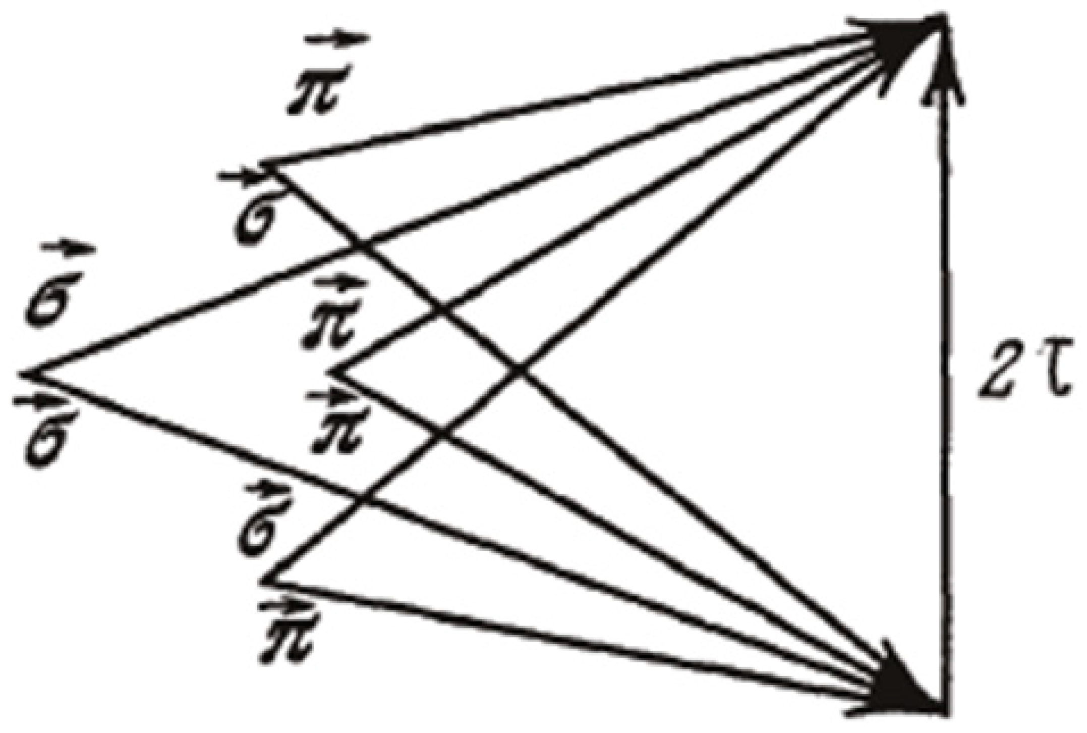
A detailed analysis of the eigen waves in CLC, in particular, their polarizations performed in [6,15], showed that four pairs of equations described by (3) correspond to four linear polarizations combinations in the second order diffraction scattering relating to slightly different diffraction angles. This polarization splitting of the diffraction angles is illustrated at Figure 1.

In the case of a CLC layer with its surfaces being perpendicular to the helical axis (see Figure 2), the second order Bragg condition relates to the parallel to τ (normal) components of the wave vectors entering in (1) and normal components of the wave vectors for the diffracting eigent-waves are determined by the Formula (1) with q determined by the formula

q = (τ/2)[(α_p)² − (F_pq)²]^½

(4)

where α_p = τ(τ + 2k_p)/k_p² is the parameter determining deviation of the wave vector from the Bragg condition and 2θ is the angle between the wave vectors of two plane waves in the eigen wave (1), and p numerates the polarization combinations shown at the Figure 1. The ratio of amplitudes (E⁻/E⁺) in the two diffracting eigen waves determined by the Equation (3) is given by the expression

ξ^± = (E⁻/E⁺)_± = F_pq/{α_p ± [(α_p)² − (F_pq)²]^½}

(5)

Note that the general expression for parameter α = τ(τ + 2k)/k² reduces to α = 2(Δω/ω_B)sinθ_B for a changing the frequency by Δω at a fixed incidence angle and to α = 2ΔθsinθB for a changing the the incidence angle by Δθ at a fixed frequency, where ω_B and θ_B are the Bragg frequency and the Bragg angle, respectively.

3. Boundary Problem in Noncollinear Geometry

A consideration of the boundary problem in the formulation which assumes that a plane optical wave of diffracting polarization is obliquely incident at a planar CLC layer. The amplitudes of the two eigen waves E_±⁺ and E_±⁻ excited in the layer by the incident wave (with the amplitude of incident wave equal to unity and a propagation direction close to the one determined by a wave vector in the CLC eigen wave) are determined by the following equations

E₊⁺ + E₋⁺ = 1
exp[i K^t−₊L]ξ⁺E₊⁺ + exp[iK^t−₋L]ξ⁻E₋⁺ = 0

(6)

where L is the layer thickness.

The amplitude reflection R_a and transmission T_a coefficients for light of diffracting polarization (π or σ) take the form:

R_a = −iF_pp(sinq_pL)/[(2q_p/τ)cosq_pL − iαpsinq_pL]
T_a = (2q_p/τ)exp[iτL/2]/[(2q_p/τ)cosq_pL − iα_psinq_pL]

(7)

The reflection R = |R_a|² and transmission T = |T_a|² coefficients experience oscillations versus the frequency outside the stop-band. In non-absorbing layers the relation R + T = 1 holds for all frequencies. At q_p = nπ/L, where n is an integer number, R = 0 and T = 1.

As it is known [13], the dispersion equation for an edge mode can be obtained as a condition of solvability of the homogeneous equation obtained from Equation (6), i.e., zero value of the Equation (6) determinant:

tg(q_pL) = −2i(q_p/τ)/α_p

(8)

In a general case, the solution of Equation (8) determining the second order CEM frequencies (ω_CEM) can be found only numerically. The CEM frequencies ω_CEM occur to be complex quantities which may be presented as ω_CEM = ω⁰_CEM(1 + iΔ), where Δ in real situations is a small parameter. So, the localized modes are weakly decaying in time, i.e., they are quasi-stationary modes. Luckily, an analytic solution can be found for some limiting case, namely, for a sufficiently small Δ ensuring the condition (qL)Im(q/2τ) << 1. In this case the values of a real part of ω_CEM, i.e., ω⁰_CEM, are coinciding with the frequencies of zero values of reflection coefficient R for a non-absorbing layer and the complex CEM frequencies are determined by the relations:

(Lq) = nπ, Δ = −(1/2)F_pp(nπ)²/[F_ppLτ/2]³

(9)

where n is an integer number numerating CEMs.

The CEM life-time in this limiting case is

τ_CEM ≈ (Lε₀^½/c)[2LF_pp/pn]²

(10)

where c is the speed of light.

In the found solution of the homogeneous system (6), the eigen solutions amplitude ratio is −1 and the electromagnetic field inside the layer is a superposition of two eigen waves of the form determined by Equation (1) with the amplitude ratio E₋⁺/E₊⁺ = −1.

The following from (1) expression for the electromagnetic field inside the layer is given by the formula

E(z,r_┴,t) = exp[i(r_┴kcosθ − ω_nt)][2σ₊iexp(iτz)sin(q_nz) + σ₋exp(−iτz)(ξ_n⁺exp(iq_nz) − ξ_n⁻exp(−iq_nz))]

(11)

where ω_n, is the nth CEM frequency and q_n, ξ_n^±, are determined by the dispersion Equations (8) and (5), respectively, and r_┴ is the radius-vector parallel to the layer surface. In the limiting case of (qL)Im(q/τ) << 1 the q_n is determined by the Expession (9) and the Expression (11) reduces to the simple formula:

E(z,r_┴,t) = exp[i(r_┴kcosθ − ω_nt)][2σ₊iexp(iτz)sin(nπz/L) + σ₋exp(−iτz)(ξ_n⁺exp(inπz/L) − ξ_n⁻exp(−i nπz/L))]

(12)

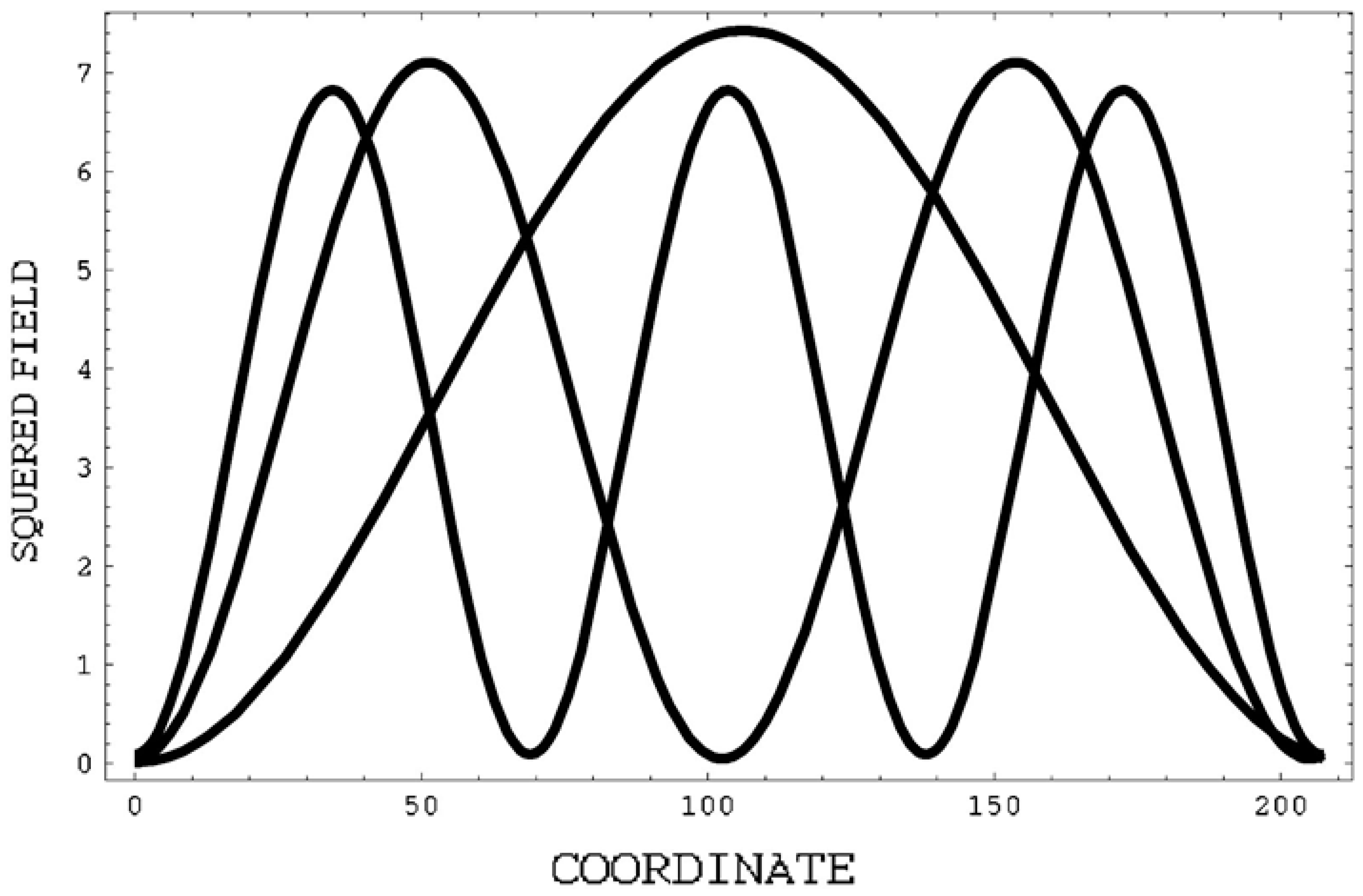
The (11) and (12) eigen solution of the boundary problem is a localized at the layer thickness L standing wave with a modulation along the z amplitude. The number of modulation periods at the layer thickness L is coinciding with the CEM number n. The CEM energy density distributions along the normal following from Equation (12) for the CEM numbers n = 1,2,3 are presented at Figure 3. Figure 3 presents a total energy density distribution in the layer along the normal to its surfaces for the cases σ-π and π-σ polarizations of individual plane waves in their eigen waves. In the cases σ-σ and π-π polarizations of individual plane waves the CEM energy density is modulated by frequent beats with the period equal to p/2 and the distribution shape accept the form presented in Figure 3 after an averaging over the beat period.

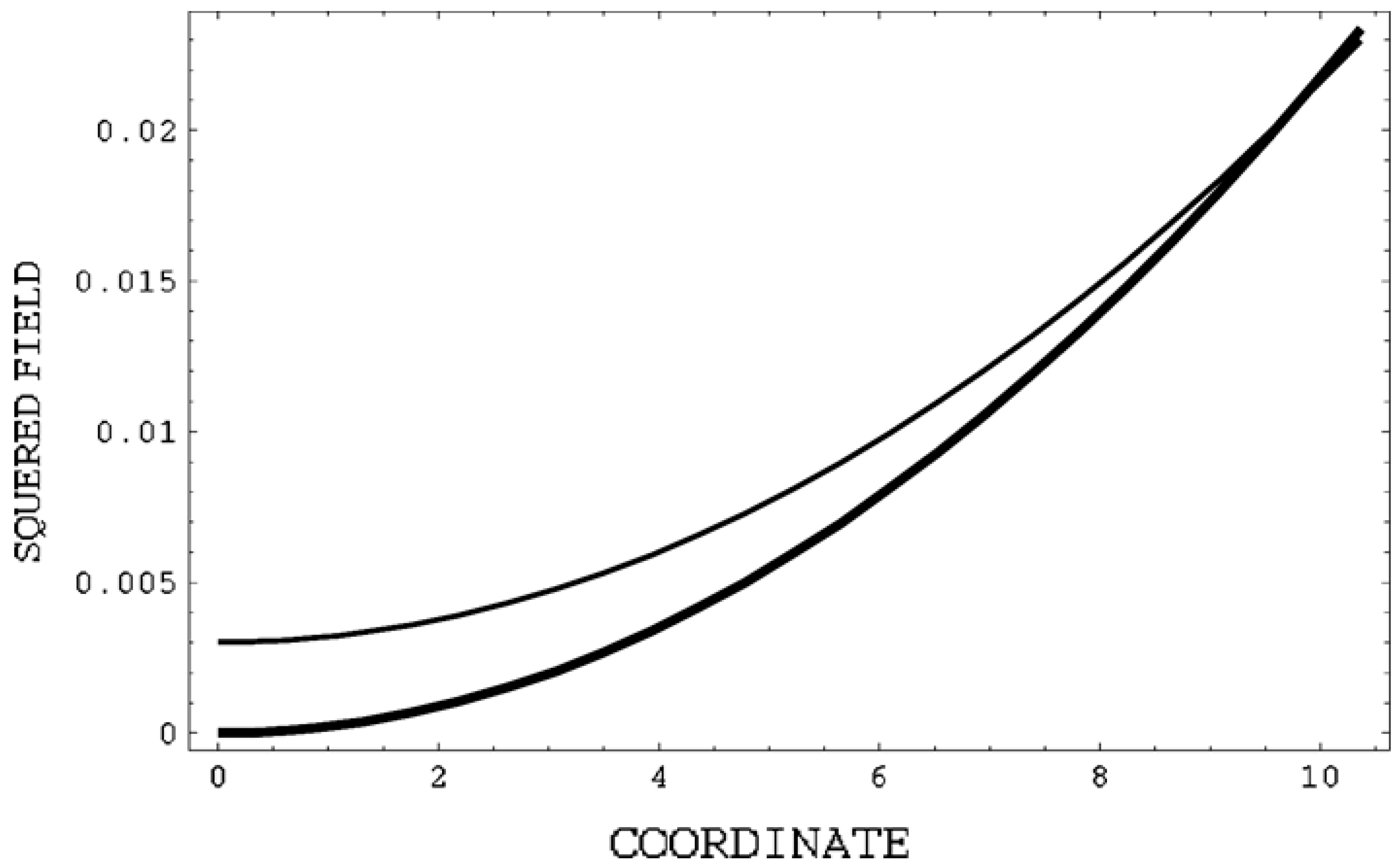
However, in each point of the layer, the total density is presented by two plane waves propagating in different directions, so one can calculate separately for any point in the layer the intensities of waves propagating in different directions. Figure 4 shows the energy density coordinate distributions of the waves propagating inside and outside of the layer close to the layer surfaces.

One can see that, at the layer surface, the energy density of the wave propagating inside the layer is strictly zero, however, for the same point, the energy density of the wave propagating outside the layer is not zero, but small. It means that the CEM energy is leaking from the layer through its surfaces. The expression for the leaking wave amplitude at the layer surface follows from Equation (12) and for [F_pqLτ/2] >> 1 looks as

|E_out| ≈ nπ/(2τLF_pq)

(13)

For sufficiently thick layers, the CEM life-time τ_m grows as a third power of the thickness for growing their thickness L and is inversely proportional to the square of the CEM number n (see (10)).

4. Absorbing CLC

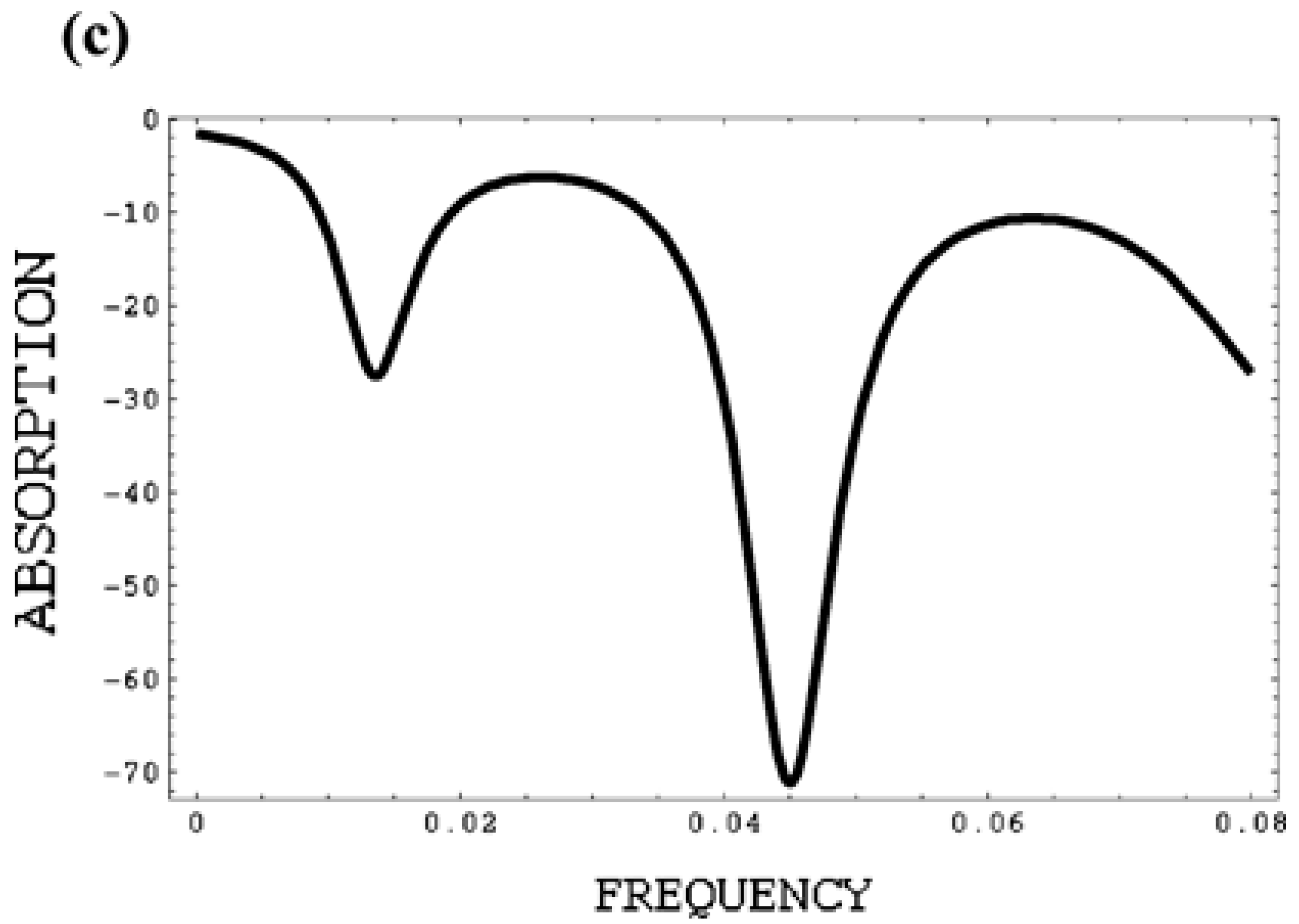
Let us examine now a second order CEM in absorbing CLC. The motivation of this study, in particular, is due to the anomalously strong absorption effect known in photonics [16,17]. Examine in more detail the formulas of the preceding sections assuming for simplicity that the absorption in the layer is isotropic. The absorption of an optical wave results in the appearance of an imaginary part in the wave vector. Define the ratio of the wave vector imaginary part to its real part as γ, i.e., k = k₀ (1 + iγ), where k₀ is the real part of wave vector. Note, that in the actual situations γ << 1. At Figure 5, 1-R-T (total absorption) calculated versus the real part of the wave vector are presented for several values of positive γ.

The absorption reveals energy beats close to the edge of the selective reflection band with maxima positions coinciding with the locations of R minima. The simplest situation corresponds to the case of a >> 1 where a = F_pqπL/p.

For a small γ and (τL)Im(2q/τ} << 1, the following from Equation (7) intensity reflection, transmission coefficients and total absorption at the frequencies of reflection minima (11) are reduced to the following expressions:

R = (a³ γ/F_pq)²/[(nπ)² + a³ γ/F_pq)]²

T = (nπ)⁴/[[(nπ)² + a³ γ/F_pq]²

(14)

1 − (R + T) = [2(nπ)²a³ γ/F_pq]/[(nπ)² + a³ γ/F_pq]²

It follows from (14) that for each n maximal absorption, i.e., the maximal 1-R-T, occurs for (nπ)² = a³ γF_pq. It means that a maximal absorption occurs for a special relationship between n, γ, the propagation direction and L and if this relationship, i.e., (nπ)² = a³γ/F_pq, is fulfilled R = 1/4, T = 1/4 and 1-R-T = 1/2.

Because the assumed smallness of γ, this result corresponds to a strong enhancement of the absorption for weakly absorbing layers. The absorption enhancement may be observed by directly measuring of 1-R-T. However, from the experimental point of view, the measuring of the intensity of some inelastic process is easier; for example, the measuring of the secondary produced fluorescence intensity. The anomalously strong absorption may be used for CEM detection, however, the most efficient detection demands special interconnection of the problem parameters. In fact, as Equation (14) shows, the absorption maximum corresponds to (nπ)² = 2a³γ/δ(1 + sinθ). Because γ is determined by the layer substance, for the maximum absorption, a special relation between the propagation direction, period, layer thickness and the amplitude of effective dielectric constant modulation has to be fulfilled to ensure the equality

γ = (πn)²/[F_pq² (2πL/p)³]

(15)

For the cases of π-σ and σ-π polarizations Equation (15) gives the following dependence of γ ensuring a maximal absorption on the CLC local anisotropy, scattering angle and the CLC thickness: γ = (2n²/πδ)(p/δL)³ (sin²θ)/cos⁴θ.

5. Amplifying LC

We now assume that γ < 0, which means that the CLC is amplifying. If |γ| is sufficiently small, the waves emerging from the layer according to Equation (6) exist only in the presence of at least one external wave incident on the layer, and their amplitudes are determined by the solution of Equation (6), i.e., by Equation (7). In this case (see Figure 6c) R + T > 1 or 1-R-T < 0 which just corresponds to the definition of an amplifying medium.

However, if the imaginary part of the dielectric tensor, i.e., γ, reaches some critical negative value, the quantity R+T diverges and the amplitudes of waves emerging from the layer are nonzero even for zero amplitudes of the incident waves. This happens when the determinant of Equation (6) reaches zero value. At this point, of course, the amplitudes of emerging waves are not determined by the solution (7) of linear equations (a nonlinear problem should then be solved). As we saw above, the points of reducing the determinant of Equation (6) to zero determine the CEM frequencies and the corresponding values of the gain (or the negative imaginary part of the dielectric tensor), i.e., the minimum threshold gain at which the conic lasing occurs (see the corresponding discussion for EM in spiral and scalar periodic media in Ref. [18,19,20]).

Therefore, the equation determining the threshold gain (γ) at which the lasing occurs (zero value of the determinant of Equation (6) or of the denominator in (7)) turns out to be coinciding with Equation (8), but it should be solved now not for the frequency but for the imaginary part of the dielectric constant (γ). In the general case, this equation has to be solved numerically. However, for a very small negative imaginary part of the dielectric tensor, the CEM frequency values are pinned to the frequencies of the reflection coefficient minima in its frequency beats outside the stop-band edge or to the reflection zero for the same layer with a zero imaginary part of the dielectric tensor [18,21,22]. This is why the threshold values of the gain for the CEM can be represented by analytic expressions in this limit case.

The threshold values of γ for a lasing at the second order CEM frequencies (i.e., a minimum |γ| at which the lasing occurs for n-th reflection minimum) corresponds to:

γ = −(nπ)²/[F_pq²(Lτ/2)³]

(16)

For the cases of π-σ and σ-π polarizations Equation (16) gives the following dependence of γ on the CLC local anisotropy, scattering angle and the CLC thickness: γ = −(2n²/πδ)(p/δL)³ (sin²θ)/cos⁴θ.

As can be seen from (16), the threshold values of |γ| are inversely proportional to the third power of the layer thickness and increase with the angle θ decrease and a minimal value of |γ| corresponds to n = 1, i.e., to the CEM frequency closest to the selective reflection band edge (cf. analogous results for EM in a scalar layered media [19,20]). The value of γ given by Equation (16) is convenient to use for an estimating the threshold values of γ in the general case and as a zero approximation in the numerical solution of Equation (8) for the threshold values of γ.

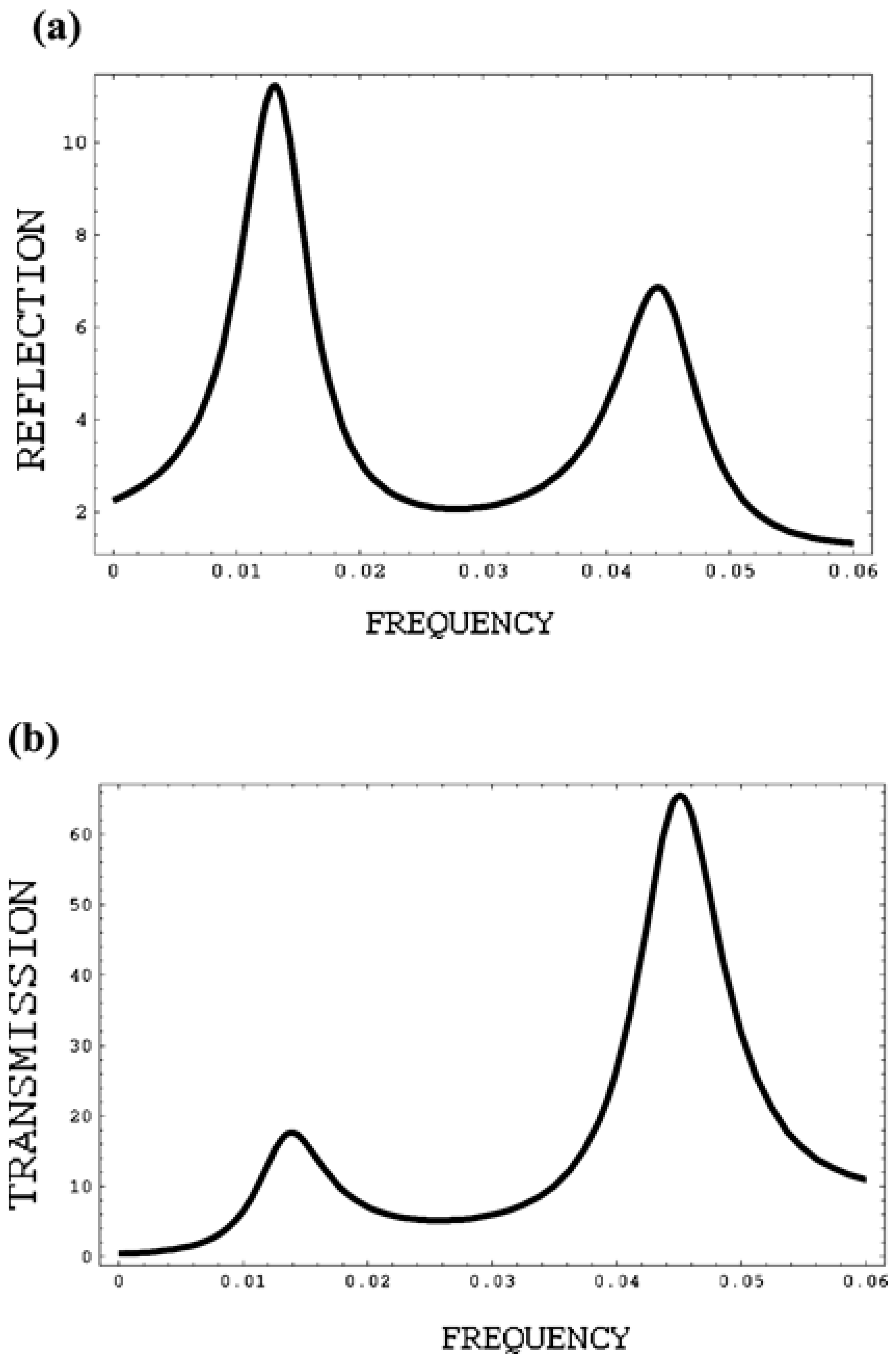
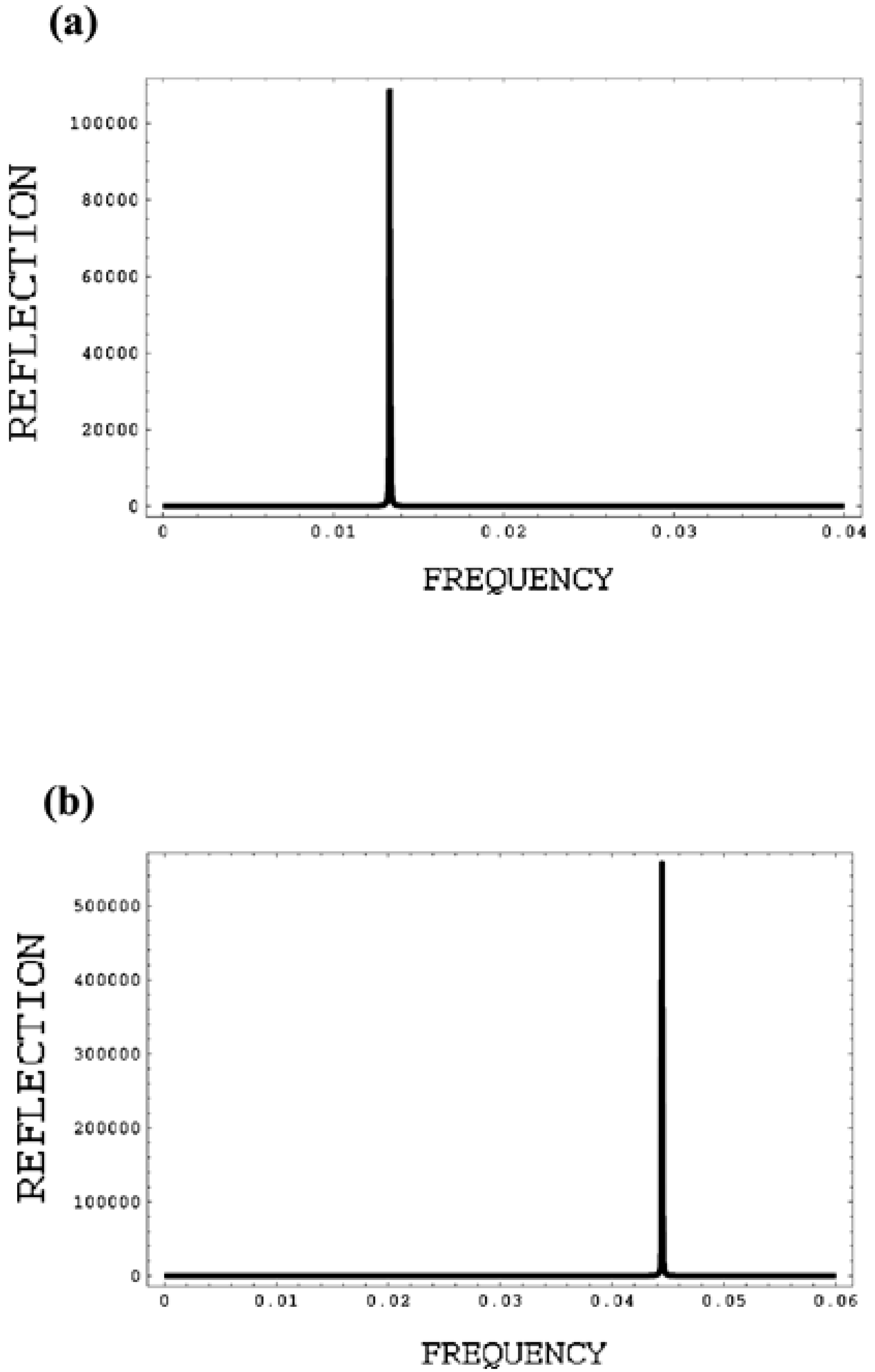
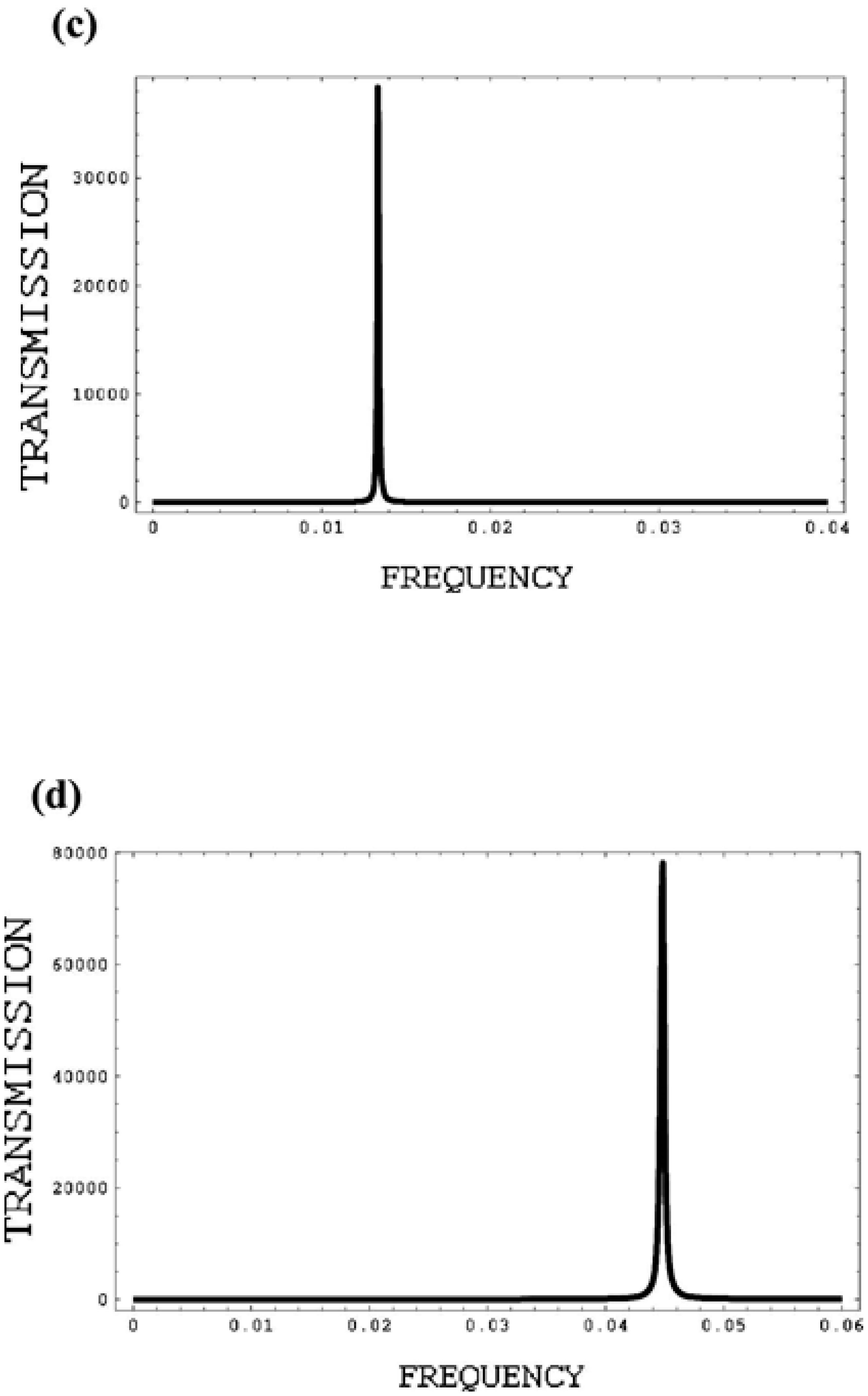
It also follows from Figure 6 that different threshold values of γ (at divergent R and T) correspond to the different CEM numbers n in Figure 7a–d. This means that individual lasing modes can be excited by changing the gain (γ). If the value of γ is between the consequent threshold values of γ for neighboring CEM, the lasing may not be achieved and the layer may reveal only amplifying properties (see Figure 6a–c). This means that changing the pumping wave intensity allows to achieve a lasing at the individual CEM, and that the lasing intensity is not a monotonic function of the pumping intensity. Because the lasing frequencies are determined by the CEM frequencies, there is an option for some variation of the lasing frequency and the CEM number inside the width of the dye line by changing the CLC pitch or by variation of the angle θ. Calculations results presented in Figure 6 and Figure 7 demonstrate that the lasing frequencies are dependent on the CLC layer parameters (like in the case of absorbing CLC, see Figure 5) in a nontrivial way. For example, an increase of the pumping power, i.e., an increase of |γ|, can result in lasing suppression.

The above results show that, qualitatively, the second order CEM properties are very similar to the EM (localized mode in a collinear geometry) ones. EM effects (anomalously strong absorption, low DFB lasing threshold etc.) also exist for CEMs. However, there are some essential differences related, first of all, to the CEM eigen mode polarizations and to a more weak than for EM realization of the mentioned above effects. In particular, the DFB lasing threshold is higher for the second order CEM in comparison with EM. It is a direct consequence of the fact that, in the equations determining the lasing threshold for the second order CEM instead δδ, entering for EM, enters a smaller quantity proportional to δ² (see (3)). So, consequently, the more propagation direction deviation form the normal to the layer the higher lasing threshold for CEM. This explains an easier obtaining of EM (collinear) lasing compared to the CEM lasing in the experiment.

6. Conclusions

The above analytic description of the second order CEM is approximate (based at the two-wave dynamical diffraction theory), however, for many cases, it may be regarded as exact from a practical point of view, because the accuracy of results is determined by a small parameter δ². If the experiment demands higher accuracy, the solution obtained in the framework of the presented approach may be regarded as a zero approximation in subsequent numerical calculations. What is concerning of the qualitative results, without doubt, is that they are correctly described in the present approach. The said relates to the conclusion that the lasing threshold for the second order CEM is higher than for EM (collinear lasing geometry). Regarding the second order CEM polarization properties, the predicted linear π and σ polarizations can be directly verified in the experiment. Difficulties in the experimental observation of a second order CEM look as not very serious because the diffraction scattering of the second order in CLC was observed many years ago [23,24]. The DFB lasing at the second order CEM frequencies demands CLCs with a large local dielectric anisotropy δ for a lowering of the lasing threshold. Detailed formulas were presented above for the second order CEM only. The physics and formulas for a CEM of diffraction order higher than 2 are similar to the ones for the second order differing only by the power of δ and the numerical factor in the corresponding expressions (instead δ² should be used δ^s for the sth diffraction order) [6].

The obtained analytical results can be easily applied to the CEM in scalar photonic media. Some general properties of CEM should also be mentioned. These are localized at the layer thickness (in one dimension) modes (electromagnetic structures) propagating along the layer surface with a propagation speed depending on the structure deviation from the collinear geometry (angle θ). So, if the EM is a motionless electromagnetic structure, the CEM is moving along the layer surface electromagnetic structure with a phase velocity equal to ccosθ. So, this property can be a base for the CEMs’ apparent using in time-delay lines for light.

A direct use of the presented analytical results on CEM may be their application to many experimental observations of conical edge modes (see [9,10,11,12,13]) for clarification of the observed phenomena physics and formulating optimal conditions for observation and application of the corresponding effects.

The work is supported by the State Assignment “0033-2019-0001”.

References

- Yang, Y.-C.; Kee, C.-S.; Kim, J.-E.; Park, H.Y.; Lee, J.C.; Jeon, Y.J. Photonic defect modes of cholesteric liquid crystals. Phys. Rev. E 1999, 60, 6852. [Google Scholar] [CrossRef] [PubMed]
- Kopp, V.I.; Genack, A.Z. Double-helix chiral fibers. Phys. Rev. Lett. 2003, 89, 033901. [Google Scholar] [CrossRef] [PubMed]
- Schmidtke, J.; Stille, W.; Finkelmann, H. Defect mode emission of a dye doped cholesteric polymer network. Phys. Rev. Lett. 2003, 90, 083902. [Google Scholar] [CrossRef] [PubMed]
- Shibaev, P.V.; Kopp, V.I.; Genack, A.Z. Photonic materials based on mixtures of cholesteric liquid crystals with polymers. J. Phys. Chem. B 2003, 107, 6961. [Google Scholar] [CrossRef]
- Ortega, J.; Folcia, C.L.; Etxebarria, J. Laser emission at the second-order photonic band gap in an electric-field-distorted cholesteric liquid crystal. Liq. Cryst. 2019. [Google Scholar] [CrossRef]
- Belyakov, V.A. Diffraction Optics of Complex Structured Periodic Media (Localized Optical Modes of Spiral Media); Springer: Berlin, Germany, 2019; Chapters 3–5. [Google Scholar]
- Belyakov, V.A. Localized Conical Edge Modes of Higher Orders in Photonic Liquid Crystals. Crystals 2019, in press. [Google Scholar]
- Yablonovitch, E.; Gmitter, T.J.; Meade, R.D.; Rappe, A.M.; Brommer, K.D.; Joannopoulos, J.D. Donor and acceptor modes in photonic band structure. Phys. Rev. Lett. 1991, 67, 3380. [Google Scholar] [CrossRef] [PubMed]
- Lee, C.-R.; Lin, S.-H.; Yeh, H.-C.; Ji, T.D.; Lin, K.L.; Mo, T.S.; Kuo, C.T.; Lo, K.Y.; Chang, S.H.; Fuh, A.Y.; et al. Color cone lasing emission in a dye-doped cholesteric liquid crystal with a single pitch. Opt. Express 2009, 17, 1290. [Google Scholar] [CrossRef] [PubMed]
- Lee, C.R.; Lin, S.H.; Ku, H.S.; Liu, J.H.; Yang, P.C.; Huang, C.Y.; Yeh, H.C.; Ji, T.D.; Lin, C.H. Spatially band-tunable color-cone lasing emission in a dye-doped cholesteric liquid crystal with a photoisomerizable chiral dopant. Appl. Phys. Lett. 2010, 96, 111105. [Google Scholar] [CrossRef]
- Lin, S.-H.; Lee, C.-R. Novel dye-doped cholesteric liquid crystal cone lasers with various birefringences and associated tunabilities of lasing feature and performance. Opt. Express 2011, 19, 18199. [Google Scholar] [CrossRef] [PubMed]
- Ying, C.-F.; Zhou, W.-Y.; Li, Y.; Ye, Q.; Yang, N.; Tian, J.-G. Multiple and colorful cone-shaped lasing induced by band-coupling in a 1D dual-periodic photonic crystal. AIP Adv. 2013, 3, 022125. [Google Scholar] [CrossRef] [Green Version]
- César, L.; Folcia, J.O.; Etxebarria, J. Cone-Shaped Emissions in Cholesteric Liquid Crystal Lasers: The Role of Anomalous Scattering in Photonic Structures. ACS Photonics 2018, 5, 4545–4553. [Google Scholar] [CrossRef]
- Belyakov, V.A.; Semenov, S.V. Optical edge modes in photonic liquid crystals. J. Exp. Theor. Phys. 2009, 109, 687–699. [Google Scholar] [CrossRef]
- Belyakov, V.A.; Dmitrienko, V.E. Optics of cholesteric liquid crystals. Sov. Phys. Solid State 1974, 15, 1811. [Google Scholar] [CrossRef]
- Belyakov, V.A.; Gevorgian, A.A.; Eritsian, O.S.; Shipov, N.V. Anomalous absorption in cholesterics. Zh. Tekhn. Fiz./Sov. Phys. Tech. Phys. 1987, 57, 843–845. [Google Scholar]
- Belyakov, V.A.; Dmitrienko, V.E. Optics of Chiral Liquid Crystals. In Soviet Scientific Reviews/Section A, Physics Reviews; Khalatnikov, I.M., Ed.; Harwood Academic Publisher: Reading, UK, 1989; Volume 13, pp. 1–203. [Google Scholar]
- Kopp, V.I.; Zhang, Z.-Q.; Genack, A.Z. Lasing in chiral photonic structures. Prog. Quant. Electron. 2003, 27, 369. [Google Scholar] [CrossRef]
- Kogelnik, H.; Shank, C.V. Coupled-wave theory of distributed feedback lasers. J. Appl. Phys. 1972, 43, 2327. [Google Scholar] [CrossRef]
- Yariv, A.; Nakamura, M. Periodic structures for integrated optics. J. Quantum Electron. 1977, 13, 233. [Google Scholar] [CrossRef]
- Shabanov, V.F.; Vetrov, S.Y.; Shabanov, A.V. Optics of Real Photonic Crystals; RAS, Sibirian Branch: Novosibirsk, Russia, 2005. (In Russian) [Google Scholar]
- Belyakov, V.A. Localized optical modes in optics of chiral liquid crystals. In New Developments in Liquid Crystals and Applications; Choudhury, P.K., Ed.; Nova Publishers: New York, NY, USA, 2013; Chapter 7; pp. 199–227. [Google Scholar]
- Berreman, D.W.; Sheffer, T.J. Bragg Reflection of Light from Single-Domain Cholesteric Liquid-Crystal Films. Phys. Rev. Lett. 1970, 25, 577. [Google Scholar] [CrossRef]
- Takezoe, Y.; Ouchi, A.; Hashimoto, K.; Masahiko, H.; Fukuda, A.; Kuze, E. Experimental study on higher order reflection by monodomain cholesteric liquid crystals. Mol. Cryst. Liq. Cryst. 1983, 101, 329. [Google Scholar] [CrossRef]
Figure 1.
Second order Bragg conditions in vector form for a CLC with a strong local birefringence.
Figure 2.
Schematic of the boundary problem for conical edge modes.
Figure 3.
Calculated second order CEM energy density (arbitrary units) for the π-σ and σ-π polarization cases versus the coordinate (in the dimensionless units 2zτ) inside the layer for the three first second order CEMs (δ2(cos2θ)/4sinθ = 0.05, N = 33, n = 1,2,3).
Figure 4.
Calculated second order CEM energy (arbitrary units) distributions for the π-σ and σ-π polarization cases close to the CLC layer surface versus coordinate (in the dimensionless units 2zτ) for a plane wave directed inside (bold line) and outside the layer for the first second order edge mode (δ2(cos2θ)/4sinθ = 0.05, N = 16.5, n = 1).
Figure 5.
Absorption in the layer (1-R-T) for the π-π polarization case calculated versus the wave vector (N = 700, δ2(cos2θ)/4 = 0.03) (a) for γ = 0.0002, (b) γ = 0.0007.
Figure 6.
R (a), T (b), 1-R-T (c) for the π-π polarization case calculated versus the frequency (l = 300, l = Lτ, δ2(cos2θ)/4 = 0.05) for γ = −0.009, i.e., for the gain between the thresholds for the first and the second edge modes.
Figure 7.
Calculated for the π-π polarization case frequency dependence of R (l = 300, l = Lτ, δ2(cos2θ)/4 = 0.05) (a) close to the threshold gain for the first second order lasing edge mode (γ = −0.00565), (b) close to the threshold gain for the second second order lasing edge mode (γ = −0.0129); calculated frequency dependence of T (l = 300, l = Lτ, δ2(cos2θ)/4 = 0.05) (c) close to the threshold gain for the first second order lasing edge mode (γ = −0.00565), and (d) close to the threshold gain for the second second order edge mode (γ = −0.0129).
© 2019 by the authors. Licensee MDPI, Basel, Switzerland. This article is an open access article distributed under the terms and conditions of the Creative Commons Attribution (CC BY) license (http://creativecommons.org/licenses/by/4.0/).
Share and Cite
MDPI and ACS Style
Belyakov, V.A.; Semenov, S.V. Localized Conical Edge Modes of Higher Orders in Photonic Liquid Crystals. Crystals 2019, 9, 542. https://0-doi-org.brum.beds.ac.uk/10.3390/cryst9100542
AMA Style
Belyakov VA, Semenov SV. Localized Conical Edge Modes of Higher Orders in Photonic Liquid Crystals. Crystals. 2019; 9(10):542. https://0-doi-org.brum.beds.ac.uk/10.3390/cryst9100542
Chicago/Turabian StyleBelyakov, Vladimir A., and Sergei V. Semenov. 2019. "Localized Conical Edge Modes of Higher Orders in Photonic Liquid Crystals" Crystals 9, no. 10: 542. https://0-doi-org.brum.beds.ac.uk/10.3390/cryst9100542
Note that from the first issue of 2016, this journal uses article numbers instead of page numbers. See further details here.