Analytic Solutions to Two-Dimensional Decagonal Quasicrystals with Defects Using Complex Potential Theory

Abstract

An analytical treatment for two-dimensional point group 10 mm decagonal quasicrystals with defects was suggested based on the complex potential method. On the basis of the assumption of linear elasticity, two new conformal maps were applied to two examples: the first was an arc with an elliptic notch inner surface in a decagonal quasicrystal, where the complex potentials could be exactly obtained; and the second was concerned with a decagonal point group 10 mm quasicrystalline strip weakened by a Griffith crack, which was subjected to a pair of uniform static pressures. Using the basic idea underlying crack theory, the extent of the stress intensity factors was analytically estimated. If the height was allowed to approach infinity, these results can be turned into the known results of an “ordinary” crystal with only phonon elastic parameters when the phason and phonon-phason elastic constants are eliminated.

1. Introduction

Quasicrystal is a new structure as well as a novel material that has presented an important application prospect in engineering [1]. Quasicrystals are brittle at low and intermediate temperature, and the structural integrity requires materials to have a sufficient strength and toughness for engineering applications. Hence, the study of the crack and fracture problems of the material is significant. It is well-known that the deformation of quasicrystals is governed by two different displacement fields: one is the phonon field, which is similar to the conventional displacement field $u(u_x,u_y,u_z)$ under the long-wave length approximation; and the other is the phason field $w(w_x,w_y,w_z)$, which is an unusual physical quantity compared to the traditional condensed matter physics and materials science [2,3,4,5,6,7,8,9]. The elasticity of quasicrystals is more difficult to determine than the elasticity of crystals or classical elasticity [2,3,4,5,6,7,8,9]. To investigate the notch/crack and fracture problems of the material, Fan introduced a mathematical theory of the elasticity of quasicrystals, where one of the mathematical theories can be found in his recently published monograph [10]. In the over 200 individual quasicrystals observed to date, there are about 70 individual quasicrystals belonging to two-dimensional decagonal quasicrystals. Therefore, these kinds of quasicrystals are very important from a fundamental point and from their applications. In this study, we focused on the discussion of this class of quasicrystal. In order to measure some of the fracture parameters of the material, some scientists have acquired the fracture parameters by using the experimental specimens [4,5,6,7,8]. Recently, Mariano and his co-workers, on the basis of first invariance principles and within the framework of the (both finite and small strain) continuum mechanics of quasicrystals, have discussed the steady crack propagation and dislocation of the quasicrystals [11,12,13]. In addition, Wang et al. studied quasicrystals by experimental observation and pointed out that the long-period structure in magnesium alloys as well as the precipitation of the quasicrystalline phase were very important areas of this research [14]. Li et al. [15,16], Gao [17], Li et al. [18], and Li [19,20] studied many cracked quasicrystals by adopting a variety of methods. Of course, many studies on quasicrystals can be found in [21,22,23,24,25,26,27], amongst others.

Notch/crack problems for conventional structural materials were studied by Muskhelishvili [28] in terms of complex analysis. In the present case, we studied the problem for quasicrystals governed by the quadruple harmonic equation. Therefore, the mathematical solution is much more complicated than for conventional structural and foam materials. Later, we introduce the complex analysis developed in monograph [10]. Here, we further developed the complex analysis for so-called Saint-Venant problems of quasicrystalline materials, which may extend the methodology to more worthwhile engineering applications.

2. Governing Equations of Elasticity of Decagonal Quasicrystals

Consider a plane in two-dimensional quasicrystals, and assume that it is perpendicular to the periodic symmetrical axis (e.g., axis $z$). In this case, the phonon and phason fields are respectively:

$$u=(u_x,u_y,u_z), w=(w_x,w_y,0)$$

(1)

The strain field associated with the phonon displacement field and phason field is respectively defined by [7]:

$${\epsilon }_{ij}=\frac{1}{2}(\frac{\partial u_i}{\partial x_j}+\frac{\partial u_j}{\partial x_i}), w_{ij}=\frac{\partial w_i}{\partial x_j}$$

(2)

Here, we considered only the plane problem. It was assumed that all variables were independent of $z$, i.e., the deformation is limited in a plane perpendicular to the z-axis, and this leads to ${\epsilon }_{zz}={\epsilon }_{xz}={\epsilon }_{yz}=0$. Furthermore, we can obtain the strains $w_{zz}=w_{zx}=w_{xz}=w_{zy}=w_{yz}=0$.

If we denote ${\sigma }_{ij}$ as the stress tensor associated to the strain tensor ${\epsilon }_{ij}$ and $H_{ij}$ as the stress tensor associated with the strain tensor $w_{ij}$, then the generalized Hooke’s law for decagonal quasicrystals with $10mm$ point groups can be expressed by [7]:

$$\{\begin{array}{l}{\sigma }_{xx}=L({\epsilon }_{xx}+{\epsilon }_{yy})+2M{\epsilon }_{xx}+R(w_{xx}+w_{yy})\\ {\sigma }_{yy}=L({\epsilon }_{xx}+{\epsilon }_{yy})+2M{\epsilon }_{yy}-R(w_{xx}+w_{yy})\\ {\sigma }_{xy}={\sigma }_{yx}=2M{\epsilon }_{xy}+R(w_{yx}-w_{xy})\\ H_{xx}=K_1{w}_{xx}+K_2{w}_{yy}+R({\epsilon }_{xx}-{\epsilon }_{yy})\\ H_{yy}=K_1{w}_{yy}+K_2{w}_{xx}+R({\epsilon }_{xx}-{\epsilon }_{yy})\\ H_{xy}=K_1{w}_{xy}-K_2{w}_{yx}-2R{\epsilon }_{xy}\\ H_{yx}=K_1{w}_{yx}-K_2{w}_{xy}+2R{\epsilon }_{xy}\end{array}$$

(3)

where $L=C_{12},M=(C_{11}-C_{12})/2=C_{66}$; $C_{ij}$ represents the phonon elastic constants; $K_i$ represents the phason elastic constants; and $R$ is the phonon–phason coupling elastic constant. In addition, the equilibrium equations are as follows:

$$\begin{array}{ll}\frac{\partial {\sigma }_{xx}}{\partial x}+\frac{\partial {\sigma }_{xy}}{\partial y}=0,& \frac{\partial {\sigma }_{yx}}{\partial x}+\frac{\partial {\sigma }_{yy}}{\partial y}=0\\ \frac{\partial H_{xx}}{\partial x}+\frac{\partial H_{xy}}{\partial y}=0,& \frac{\partial H_{yx}}{\partial x}+\frac{\partial H_{yy}}{\partial y}=0\end{array}\}$$

(4)

Equations (2)–(4) are the basic equations describing the elasticity of decagonal quasicrystals under plane deformation, and this is an equation made of 18 field equations.

Based on the deformation compatibility equations,

$$\frac{{\partial }^2{\epsilon }_{xx}}{\partial y^2}+\frac{{\partial }^2{\epsilon }_{yy}}{\partial x^2}=2\frac{{\partial }^2{\epsilon }_{xy}}{\partial x\partial y}, \frac{\partial w_{xx}}{\partial y}=\frac{\partial w_{xy}}{\partial x}, \frac{\partial w_{yy}}{\partial x}=\frac{\partial w_{yx}}{\partial y}$$

(5)

If we introduce the three functions $\varphi (x,y)$, ${\psi }_1(x,y)$, and ${\psi }_2(x,y)$, as follows:

$$\{\begin{array}{l}{\sigma }_{xx}=\frac{{\partial }^2\varphi }{\partial y^2},\hspace{1em}{\sigma }_{yy}=\frac{{\partial }^2\varphi }{\partial x^2},\hspace{1em}{\sigma }_{xy}={\sigma }_{yx}=-\frac{{\partial }^2\varphi }{\partial x\partial y}\\ H_{xx}=\frac{\partial {\psi }_1}{\partial y},\hspace{1em}{H}_{xy}=-\frac{\partial {\psi }_1}{\partial x},\hspace{1em}{H}_{yx}=-\frac{\partial {\psi }_2}{\partial y},\hspace{1em}{H}_{yy}=\frac{\partial {\psi }_2}{\partial x}\end{array}$$

(6)

Equation (5) can be transformed into the following simple forms:

$$\{\begin{array}{l}\left(\frac{1}{2(L+M)}+\frac{K_1+K_2}{2M(K_1+K_2)-4R^2}\right){\nabla }^2{\nabla }^2\varphi +\frac{R}{M(K_1+K_2)-2R^2}\left(\frac{\partial }{\partial y}{\Pi }_1{\psi }_1-\frac{\partial }{\partial x}{\Pi }_2{\psi }_2\right)=0\\ \left(\frac{1}{K_1-K_2}+M\right){\nabla }^2{\psi }_1+R\frac{\partial }{\partial y}{\Pi }_1\varphi =0\\ \left(\frac{1}{K_1-K_2}+M\right){\nabla }^2{\psi }_2-R\frac{\partial }{\partial x}{\Pi }_2\varphi =0\end{array}$$

(7)

where ${\nabla }^2=\frac{{\partial }^2}{\partial x^2}+\frac{{\partial }^2}{\partial y^2}$ is the two-dimensional Laplacian operator, and ${\Pi }_1=3\frac{{\partial }^2}{\partial x^2}-\frac{{\partial }^2}{\partial y^2}$, ${\Pi }_2=3\frac{{\partial }^2}{\partial y^2}-\frac{{\partial }^2}{\partial x^2}$. When we let the three functions $\varphi (x,y)$, ${\psi }_1(x,y)$, and ${\psi }_2(x,y)$, so that:

$$\varphi =c_1{\nabla }^2{\nabla }^{2}G, {\psi }_1=-(R\frac{\partial }{\partial y}{\Pi }_1){\nabla }^{2}G, {\psi }_2=(R\frac{\partial }{\partial x}{\Pi }_2){\nabla }^{2}G$$

(8)

then the Equation (7) set can be reduced to a unique equation of a higher order, i.e., the potential function $G(x,y)$ satisfies the quadruple harmonic equation as follows [10]:

$${\nabla }^2{\nabla }^2{\nabla }^2{\nabla }^{2}G=0$$

(9)

where the constant is defined by $c_1=\frac{2(M{K}_1-R^2)}{K_1-K_2}$.

By introducing a complex variable, the solution of Equation (9) can be expressed as [10]:

$$G=2\mathrm{Re}[g_1(z)+\overline{z}{g}_2(z)+\frac{1}{2}{\overline{z}}^2{g}_3(z)+\frac{1}{6}{\overline{z}}^3{g}_4(z)]$$

(10)

where $g_j(z) (j=1, 2, 3, 4)$ are four analytic functions of a single complex variable $z\equiv x+iy=r{e}^{i\theta }$. The bar denotes the complex conjugate hereinafter, i.e., $\overline{z}=x-iy=r{e}^{-}{}^{i\theta }.$ These analytic functions will be determined by the boundary conditions of practical problems. It is easy to prove that $g_1(z)$ has no contribution to the stress and displacement fields, so $g_1(z)=0$.

From the fundamental solution of Equation (10), we can find the complex representation of the stresses as given below [10]:

$$\{\begin{array}{l}{\sigma }_{xx}=-32c_1\mathrm{Re}(\Omega (z)-2g_4^{‴}(z))\\ {\sigma }_{yy}=32c_1\mathrm{Re}(\Omega (z)+2g_4^{‴}(z))\\ {\sigma }_{xy}={\sigma }_{yx}=32c_1\mathrm{Im}\Omega (z)\\ H_{xx}=32R\mathrm{Re}({\Theta }^{\prime }(z)-\Omega (z))\\ H_{xy}=-32R\mathrm{Im}({\Theta }^{\prime }(z)+\Omega (z))\\ H_{yx}=-32R\mathrm{Im}({\Theta }^{\prime }(z)-\Omega (z))\\ H_{yy}=-32R\mathrm{Re}({\Theta }^{\prime }(z)+\Omega (z))\end{array}$$

(11)

and

$$\Theta (z)=g_2^{(\mathrm{IV})}(z)+\overline{z}{g}_3^{(\mathrm{IV})}(z)+\frac{1}{2}{\overline{z}}^2{g}_4^{(\mathrm{IV})}(z), \Omega (z)=g_3^{(\mathrm{IV})}(z)+\overline{z}{g}_4^{(\mathrm{IV})}(z)$$

(12)

where the prime, two prime, three prime, and superscript ($\mathrm{IV}$) denote the first to fourth order differentiation of $g_j(z)$ to the variable $z,$ in addition to ${\Theta }^{\prime }(z)=\raisebox{1ex}{$d\Theta (z)$}\!\left/ \!\raisebox{-1ex}{$dz$}\right.$, and it is evident that $\Theta (z)$ and $\Omega (z)$ are not analytic functions.

By some derivation from Equation (11), we have the complex representation of the displacements, as follows:

$$\{\begin{array}{l}{u}_x+i{u}_y=32(4c_1{c}_2-c_3-c_1{c}_4){g^{″}}_4(z)-32(c_1{c}_4-c_3)(\overline{{g^{‴}}_3(z)}+z\overline{{g^{‴}}_4(z)})\\ w_x+i{w}_y=\frac{32R}{K_1-K_2}\overline{\Theta (z)}\end{array}$$

(13)

and the constants can be expressed by $c_2=\frac{2(M(K_1+K_2)-R^2)+L(K_1+K_2)}{4(L+M)(M(K_1+K_2)-2R^2)}$, $c_3=\frac{R^2}{M(K_1+K_2)-R^2}$, $c_4=\frac{K_1+K_2}{M(K_1+K_2)-R^2}$; and $c_1$ has been listed in the above expression.

If we introduce the new functions for convenience, such that:

$$g_2{}^{(\mathrm{IV})}(z)=h_2(z), g_3{}^{‴}(z)=h_3(z), g_4{}^{″}(z)=h_4(z).$$

(14)

All the stress and displacement components can be rewritten by $h_i(z)(i=2,3,4)$, based on these new functions. In order not to change the stresses and displacements, the analytic functions $h_3(z)$ can be replaced by $h_3(z)+{\gamma }^{\prime }$, and $h_4(z)$ can be replaced by $h_4(z)+\frac{32(c_1{c}_4-c_3)}{32(4c_1{c}_2-c_3-c_1{c}_4)}\overline{{\gamma }^{\prime }}$ [10]. Therefore, we can obtain the complex function written in the following form:

$$\{\begin{array}{l}{h}_4(z)=d_1(X+iY)\ln z+Bz+h_4{}^0(z),\\ h_3(z)=d_2(X-iY)\ln z+(B^{\prime }+i{C}^{\prime })z+h_3{}^0(z),\\ h_2(z)=(B^{″}+i{C}^{″})z+h_2{}^0(z),\end{array}$$

(15)

where $B$, $B^{\prime }$, $C^{\prime }$, $B^{″}$, and $C^{″}$ are real constants, and $d_1$, $d_2$, $h_4{}^0(z)$, $h_3{}^0(z)$, and $h_2{}^0(z)$ can be expressed as:

$$\begin{gathered} d_1=\frac{1}{64c_1\pi \times (32(4c_1{c}_2-c_3-c_1{c}_4)+1)}, d_2=-\frac{4c_1{c}_2-c_3-c_1{c}_4}{2c_1\pi \times (32(4c_1{c}_2-c_3-c_1{c}_4)+1)}, \\ {h}_4{}^0(z)=\frac{a_1}{z}+\frac{a_2}{z^2}+\cdots \cdots , h_3{}^0(z)=\frac{b_1}{z}+\frac{b_2}{z^2}+\cdots \cdots , h_2{}^0(z)=\frac{{\gamma }_1}{z}+\frac{{\gamma }_2}{z^2}+\cdots \cdots , \end{gathered}$$

and

$$B=\frac{1}{128c_1}({\sigma }_1+{\sigma }_2), B^{\prime }+i{C}^{\prime }=-\frac{1}{64c_1}({\sigma }_1-{\sigma }_2)e^{-2i\alpha },$$

where ${\sigma }_1, {\sigma }_2$ are principal stresses at infinity, and $\alpha$ is the angle of ${\sigma }_1$ and the $x$-direction. Let $z\to \infty$, we have $H_{yy}-H_{xx}+i(H_{xy}+H_{yx})=-64(R_1+R_2)B^{″}+i{C}^{″}$, and yields $B^{″}+i{C}^{″}=\frac{1}{64(R_1+R_2)}({\sigma }_1{}^{\prime }-{\sigma }_2{}^{\prime })e^{-2i{\alpha }^{\prime }}$, where ${\sigma }_1{}^{\prime },{\sigma }_2{}^{\prime }$ are the generalized principal stresses at infinity, and ${\alpha }^{\prime }$ is the angle of ${\sigma }_1{}^{\prime }$ and the $x$-direction.

As is widely-known, Muskhelishvili [28] provided two kinds rational conformal mapping for solving plane problems of elastic materials for some complicated configurations, and the first kind of rational conformal mapping reads $z=\omega (\zeta )=R(\zeta +{\displaystyle \sum _{k=0}^n{d}_k{\zeta }^{-k}})\hspace{1em}{\displaystyle \sum _{k=0}^n\left|d_k\right|}\le 1$. This mapping can transform the exterior of the unit circle in the $\zeta$-plane into the exterior of the material with defects in the physical plane. As a result of the transformation, we can obtain the series expansion of the logarithmic item $\ln z=\ln \left[R\zeta (1+{\displaystyle \sum _{k=0}^n{d}_k{\zeta }^{-(k+1)}})\right]=\ln R+\ln \zeta +\ln (1+{\displaystyle \sum _{k=0}^n{d}_k{\zeta }^{-(k+1)}})$. As $\left|\zeta \right|>1$ outside the unit circle was noted, we can obtain ${\displaystyle \sum _{k=0}^n\left|\frac{d_k}{{\zeta }^{k+1}}\right|}<1$ and also have $\ln (1+{\displaystyle \sum _{k=0}^n{d}_k{\zeta }^{-(k+1)}})=({\displaystyle \sum _{k=0}^n{d}_k{\zeta }^{-(k+1)}})+\frac{1}{2}{({\displaystyle \sum _{k=0}^n{d}_k{\zeta }^{-(k+1)}})}^2+\cdots \cdots =f(\zeta )$, where $f(\zeta )$ is analytic outside the unit circle. In light of a similar analysis, it is very easy to obtain the following formula for each of the items $h_4^0(z)$, $h_3^0(z)$, and $h_2^0(z)$ of two dimensional decagonal quasicrystals, for example, the series expansion $\frac{a_1}{z}=\frac{a_1}{R\zeta (1+{\displaystyle \sum _{k=0}^n{d}_k{\zeta }^{-(k+1)}})}=\frac{a_1}{R\zeta }(1-{\displaystyle \sum _{k=0}^n{d}_k{\zeta }^{-(k+1)}}-\cdots \cdots )$, and so on. Substituting these results into Equation (15), we have:

$$\{\begin{array}{l}{h}_4(\zeta )=d_1(X+iY)\ln \zeta +B\omega (\zeta )+h_4{}^{\ast }(\zeta )\\ h_3(\zeta )=d_2(X-iY)\ln \zeta +(B^{\prime }+i{C}^{\prime })\omega (\zeta )+h_3{}^{\ast }(\zeta )\\ h_2(\zeta )=(B^{″}+i{C}^{″})\omega (\zeta )+h_2{}^{\ast }(\zeta )\end{array}$$

(16)

where $h_4{}^{\ast }(\zeta )={\displaystyle \sum _{n=1}^{\infty }{\alpha }_n}{\zeta }^{-n}$, $h_3{}^{\ast }(\zeta )={\displaystyle \sum _{n=1}^{\infty }{\beta }_n}{\zeta }^{-n}$, and $h_2{}^{\ast }(\zeta )={\displaystyle \sum _{n=1}^{\infty }{\gamma }_n}{\zeta }^{-n}$ are single valued analytical functions of $\left|\zeta \right|>1$. The other kind of rational conformal mapping reads $z=\omega (\zeta )=R(\frac{1}{\zeta }+{\displaystyle \sum _{k=0}^n{C}_k{\zeta }^k})\hspace{1em}{\displaystyle \sum _{k=0}^n\left|C_k\right|}\le 1$. This can transform the interior of the unit circle in the mapping plane into the exterior of the material with defects in the physical plane. Through a similar analysis with the first kind of mapping, we have:

$$\{\begin{array}{l}{\tilde{h}}_4(\zeta )=-d_1(X+iY)\ln \zeta +B\omega (\zeta )+{\tilde{h}}_4{}^{\ast }(\zeta )\\ {\tilde{h}}_3(\zeta )=-d_2(X-iY)\ln \zeta +(B^{\prime }+i{C}^{\prime })\omega (\zeta )+{\tilde{h}}_3{}^{\ast }(\zeta )\\ {\tilde{h}}_2(\zeta )=(B^{″}+i{C}^{″})\omega (\zeta )+{\tilde{h}}_2{}^{\ast }(\zeta )\end{array}$$

(17)

where ${\tilde{h}}_4{}^{\ast }(\zeta )={\displaystyle \sum _{n=1}^{\infty }{\tilde{\alpha }}_n}{\zeta }^n$, ${\tilde{h}}_3{}^{\ast }(\zeta )={\displaystyle \sum _{n=1}^{\infty }{\tilde{\beta }}_n}{\zeta }^n$, and ${\tilde{h}}_2{}^{\ast }(\zeta )={\displaystyle \sum _{n=1}^{\infty }{\tilde{\gamma }}_n}{\zeta }^n$ are single valued analytical functions of $\left|\zeta \right|<1$.

Considering the stress boundary conditions for the plane elasticity of decagonal quasicrystals in the following, we can express them as:

$$\{\begin{array}{l}{\sigma }_{xx}l+{\sigma }_{xy}m=T_x, {\sigma }_{yy}m+{\sigma }_{xy}l=T_y \hspace{1em}(x,y)\in L\\ H_{xx}l+H_{xy}m=h_x , H_{yy}m+H_{yx}l=h_y\hspace{1em}(x,y)\in L\end{array}$$

(18)

where the point $(x,y)\in L$ represents an arbitrary boundary point of a multi-connected quasicrystalline material; meanwhile, we need to consider $l=\cos (n,x)=dy/ds$ and $m=\cos (n,y)=-dx/ds$. Here, $T=(T_x,T_y)$ and $h=(h_x,h_y)$ represent the surface tractions and generalized surface tractions, respectively, and $n$ denotes the outer unit normal vector of an arbitrary boundary point.

According to Equations (11) and (15) and the boundary conditions in Equation (18), we can write the boundary conditions based on our analytic functions:

$$\{\begin{array}{l}{h}_4(z)+\overline{h_3(z)}+z\overline{h_4{}^{\prime }(z)}=\frac{i}{32c_1}{\displaystyle \int (T_x+i{T}_y})ds \hspace{1em}z\in L\\ h_4{}^{″}(z)+\overline{z}{h}_3{}^{\prime }(z)+\frac{1}{2}{\overline{z}}^2{h}_4{}^{″}(z)=\frac{i}{R_2-i{R}_1}{\displaystyle \int (h_x+i{h}_y})ds \hspace{1em}z\in L\end{array}$$

(19)

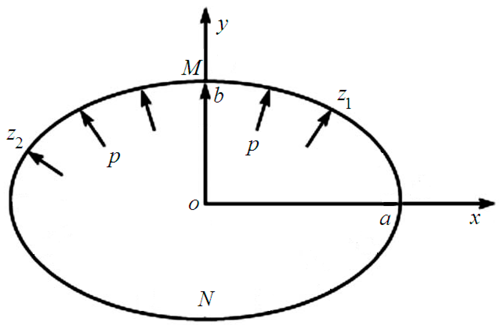
3. An Arc of Elliptic Notch Inner Surface in a Decagonal Quasicrystal

We assumed a two dimensional decagonal quasicrystal weakened by an elliptic notch $( \frac{x^2}{a^2}+\frac{y^2}{b^2}=1 )$ (see Figure 1), in which the arc $\stackrel{⌢}{z_1 M z_2}$ of the elliptic notch was subjected to a uniform pressure $p$. For this configuration and based on the above mappings, we can obtain the simplified form of the conformal mapping:

$$z=\omega (\zeta )=R(\frac{m}{\zeta }+\zeta )$$

(20)

This can transform the exterior of the unit circle in the $\zeta$-plane into the exterior of the ellipse in the z-plane, where $\zeta =\xi +i\eta =\rho e^{i\phi }$ and the constants can be expressed by $R=(a+b)/2$, $m=(a-b)/(a+b)$.

In the boundary of the unit circle, we introduce $\sigma =e^{i\theta }$ and can obtain:

$$h_4{}^{\ast }(\sigma )+\overline{h_3{}^{\ast }(\sigma )}+\frac{\omega (\sigma )}{\overline{{\omega }^{\prime }(\sigma )}}\cdot \overline{h_4{{}^{\ast }}^{\prime }(\sigma )}=f_0$$

(21)

where

$$\begin{array}{l}{f}_0=\frac{i}{32c_1}{\displaystyle \int (T_x+i{T}_y})ds-(d_1-d_2)(X+iY)\ln \sigma -\frac{\omega (\sigma )}{\overline{{\omega }^{\prime }(\sigma )}}\cdot d_1(X-iY)\cdot \sigma -\\ \hspace{1em}\hspace{1em}2B\omega (\sigma )-(B^{\prime }-i{C}^{\prime })\overline{\omega (\sigma )}.\end{array}$$

Take the conjugate on both sides of Equation (21), and it will yield:

$$\overline{h_4{}^{\ast }(\sigma )}+h_3{}^{\ast }(\sigma )+\frac{\overline{\omega (\sigma )}}{{\omega }^{\prime }(\sigma )}\cdot h_4{{}^{\ast }}^{\prime }(\sigma )=\overline{f_0}$$

(22)

If we multiply both sides of Equation (21) by $\frac{1}{2\pi i}\frac{d\sigma }{\sigma -\zeta }$, and integrate around the unit circle, then we obtain:

$$\frac{1}{2\pi i}{\displaystyle {\int }_{\gamma }\frac{h_4{}^{\ast }(\sigma )}{\sigma -\zeta }}d\sigma +\frac{1}{2\pi i}{\displaystyle {\int }_{\gamma }\frac{\omega (\sigma )}{\overline{{\omega }^{\prime }(\sigma )}}\frac{\overline{h_4{{}^{\ast }}^{\prime }(\sigma )}}{\sigma -\zeta }}d\sigma +\frac{1}{2\pi i}{\displaystyle {\int }_{\gamma }\frac{\overline{h_3{}^{\ast }(\sigma )}}{\sigma -\zeta }}d\sigma =\frac{1}{2\pi i}{\displaystyle {\int }_{\gamma }\frac{f_0}{\sigma -\zeta }}d\sigma$$

(23)

When we give the same treatment to Equation (12), we can obtain:

$$\frac{1}{2\pi i}{\displaystyle {\int }_{\gamma }\frac{\overline{h_4{}^{\ast }(\sigma )}}{\sigma -\zeta }}d\sigma +\frac{1}{2\pi i}{\displaystyle {\int }_{\gamma }\frac{\overline{\omega (\sigma )}}{{\omega }^{\prime }(\sigma )}\frac{h_4{{}^{\ast }}^{\prime }(\sigma )}{\sigma -\zeta }}d\sigma +\frac{1}{2\pi i}{\displaystyle {\int }_{\gamma }\frac{h_3{}^{\ast }(\sigma )}{\sigma -\zeta }}d\sigma =\frac{1}{2\pi i}{\displaystyle {\int }_{\gamma }\frac{\overline{f_0}}{\sigma -\zeta }}d\sigma$$

(24)

Meanwhile, according to the mapping equation $z=\omega (\zeta )=R(\frac{m}{\zeta }+\zeta )$, we can obtain these formulas based on the above mapping, i.e., $\omega (\sigma )=R(\sigma +\frac{m}{\sigma })$, $\overline{\omega (\sigma )}=R(\frac{1}{\sigma }+m\sigma )$, ${\omega }^{\prime }(\sigma )=R(1-\frac{m}{{\sigma }^2})$, and $\overline{{\omega }^{\prime }(\sigma )}=R(1-m{\sigma }^2)$. Now, we can solve Equation (23), and because $h_4{}^{\ast }(\zeta )$ is a single valued analytical function of $\left|\zeta \right|>1$, we can obtain:

$$\frac{1}{2\pi i}{\displaystyle {\int }_{\gamma }\frac{h_4{}^{\ast }(\sigma )}{\sigma -\zeta }}d\sigma =-h_4{}^{\ast }(\zeta )+h_4{}^{\ast }(\infty ), \frac{1}{2\pi i}{\displaystyle {\int }_{\gamma }\frac{\overline{h_3{}^{\ast }(\sigma )}}{\sigma -\zeta }}d\sigma =0$$

(25)

where $\frac{\omega (\zeta )}{\overline{{\omega }^{\prime }(\zeta )}}\overline{h_4{{}^{\ast }}^{\prime }(\sigma )}=\frac{({\zeta }^2+m)}{\zeta (1-m{\zeta }^2)}\left[-\overline{{\alpha }_1}{\zeta }^2-2\overline{{\alpha }_2}{\zeta }^3-\cdots \cdots \right]$ is an analytical function of $\left|\zeta \right|<1$, and we have $\frac{1}{2\pi i}{\displaystyle {\int }_{\gamma }\frac{\omega (\sigma )}{\overline{{\omega }^{\prime }(\sigma )}}\frac{\overline{h_4{{}^{\ast }}^{\prime }(\sigma )}}{\sigma -\zeta }}d\sigma =0$. Therefore, Equation (23) becomes $-h_4{}^{\ast }(\zeta )=\frac{1}{2\pi i}{\displaystyle {\int }_{\gamma }\frac{f_0}{\sigma -\zeta }}d\sigma$, where the constants are omitted. Based on the Cauchy integral basic formula for Equation (24), we have $\frac{1}{2\pi i}{\displaystyle {\int }_{\gamma }\frac{\overline{h_4{}^{\ast }(\sigma )}}{\sigma -\zeta }}d\sigma =0$ and $\frac{1}{2\pi i}{\displaystyle {\int }_{\gamma }\frac{h_3{}^{\ast }(\sigma )}{\sigma -\zeta }}d\sigma =-h_3{}^{\ast }(\zeta )+h_3{}^{\ast }(\infty )$. Meanwhile, we find that $\frac{\overline{\omega (\zeta )}}{{\omega }^{\prime }(\zeta )}{h}_4{{}^{\ast }}^{\prime }(\sigma )=\frac{\zeta (m{\zeta }^2+1)}{({\zeta }^2-m)}\left[-\frac{{\alpha }_1}{{\zeta }^2}-\frac{2{\alpha }_2}{{\zeta }^3}-\cdots \cdots \right]$ is a single valued analytical function of $\left|\zeta \right|>1$, and we have $\frac{1}{2\pi i}{\displaystyle {\int }_{\gamma }\frac{\overline{\omega (\sigma )}}{{\omega }^{\prime }(\sigma )}\frac{h_4{{}^{\ast }}^{\prime }(\sigma )}{\sigma -\zeta }}d\sigma =-\frac{\overline{\omega (\zeta )}}{{\omega }^{\prime }(\zeta )}{h}_4{{}^{\ast }}^{\prime }(\zeta )$. Therefore, Equation (24) becomes $-h_3{}^{\ast }(\zeta )-\frac{\overline{\omega (\zeta )}}{{\omega }^{\prime }(\zeta )}{h}_4{{}^{\ast }}^{\prime }(\zeta )=\frac{1}{2\pi i}{\displaystyle {\int }_{\gamma }\frac{\overline{f_0}}{\sigma -\zeta }}d\sigma$, where the constants are omitted. If we assume that the material is not subjected to force at infinity, it will lead to $B=0$ and $B^{\prime }-i{C}^{\prime }=0$. So, we have:

$$\begin{array}{l}{h}_4^{*}(\zeta )=\frac{1}{32c_1}\cdot \left[\frac{pR}{2\pi i}{\displaystyle {\int }_{{\sigma }_1}^{{\sigma }_2}(\sigma +\frac{m}{\sigma })}\frac{1}{\sigma -\zeta }d\sigma +\frac{p{z}_2}{2\pi i}{\displaystyle {\int }_{{\sigma }_2}^{{\sigma }_1}\frac{1}{\sigma -\zeta }}d\sigma \right]+\\ \hspace{1em}\hspace{1em}\hspace{1em}\frac{ip(d_1-d_2)(z_1-z_2)}{2\pi i}{\displaystyle {\int }_{\gamma }\frac{\ln \sigma }{\sigma -\zeta }}d\sigma +\frac{ip{d}_1(\overline{z_1}-\overline{z_2})}{2\pi i}{\displaystyle {\int }_{\gamma }\frac{({\sigma }^2+m)}{(1-m{\sigma }^2)}}\cdot \frac{1}{\sigma -\zeta }d\sigma \end{array}$$

(26)

where

$${\displaystyle {\int }_{{\sigma }_1}^{{\sigma }_2}(\sigma +\frac{m}{\sigma })}\frac{1}{\sigma -\zeta }d\sigma ={\sigma }_2-{\sigma }_1-\frac{m}{\zeta }\ln \frac{{\sigma }_2}{{\sigma }_1}+(\zeta +\frac{m}{\zeta })\ln \frac{{\sigma }_2-\zeta }{{\sigma }_1-\zeta }{\displaystyle {\int }_{{\sigma }_2}^{{\sigma }_1}\frac{1}{\sigma -\zeta }}d\sigma =\ln \frac{{\sigma }_1-\zeta }{{\sigma }_2-\zeta }.$$

As $\frac{({\zeta }^2+m)}{(1-m{\zeta }^2)}$ is a single valued analytic function of $\left|\zeta \right|<1$, we have ${\displaystyle {\int }_{\gamma }\frac{({\sigma }^2+m)}{(1-m{\sigma }^2)}}\cdot \frac{1}{\sigma -\zeta }d\sigma =0$. For $\frac{1}{2\pi i}{\displaystyle {\int }_{\gamma }\frac{\ln \sigma }{\sigma -\zeta }}d\sigma$, let $\frac{1}{2\pi i}{\displaystyle {\int }_{\gamma }\frac{\ln \sigma }{\sigma -\zeta }}d\sigma =I(\zeta )$, and we can obtain:

$$\begin{array}{ll}\frac{dI(\zeta )}{d\zeta }=& \frac{1}{2\pi i}{\displaystyle {\int }_{\gamma }\frac{\ln \sigma }{{(\sigma -\zeta )}^2}}d\sigma =-\frac{1}{2\pi i}{\displaystyle {\int }_{\gamma }\ln \sigma }d(\frac{1}{\sigma -\zeta })\\ & =-\frac{1}{2\pi i}{[\frac{\ln \sigma }{\sigma -\zeta }]}_{\sigma =e^{i{\phi }_1}}^{\sigma =e^{i({\phi }_1+2\pi )}}+\frac{1}{2\pi i}{\displaystyle {\int }_{\gamma }\frac{1}{\sigma (\sigma -\zeta )}}d\sigma \\ & =-\frac{1}{2\pi i}\frac{1}{{\sigma }_1-\zeta }\ln \frac{e^{i({\phi }_1+2\pi )}}{e^{i{\phi }_1}}-\frac{1}{\zeta }\\ & =-\frac{1}{{\sigma }_1-\zeta }-\frac{1}{\zeta }\end{array}$$

where ${\sigma }_1=e^{i{\phi }_1}$. Therefore, we have $\frac{1}{2\pi i}{\displaystyle {\int }_{\gamma }\frac{\ln \sigma }{\sigma -\zeta }}d\sigma =I(\zeta )=\ln ({\sigma }_1-\zeta )-\ln \zeta +C$.

Calculating the sum of the above results, and noting Equation (17), we have:

$$\begin{array}{l}{h}_4(\zeta )=\frac{1}{32c_1}\cdot \frac{p}{2\pi i}\cdot \left[-\frac{mR}{\zeta }\ln \frac{{\sigma }_2}{{\sigma }_1}+z\ln \frac{{\sigma }_2-\zeta }{{\sigma }_1-\zeta }+z_1\ln ({\sigma }_1-\zeta )-z_2\ln ({\sigma }_2-\zeta )\right]\\ \hspace{1em}\hspace{1em}\hspace{1em}+ip(d_1-d_2)(z_1-z_2)\ln \zeta \end{array}$$

(27)

Similarly, by solving Equation (24), one gets:

$$\begin{array}{l}{h}_3(\zeta )=\frac{1}{32c_1}\cdot \frac{p}{2\pi i}\cdot \left[-\frac{(1+m^2)R\zeta }{({\zeta }^2-m)}\ln \frac{{\sigma }_2}{{\sigma }_1}+\frac{R({\sigma }_1-{\sigma }_2)(1+m{\zeta }^2)}{({\zeta }^2-m)}-\overline{z_2}\ln ({\sigma }_2-\zeta )+\overline{z_1}\ln ({\sigma }_1-\zeta )\right]\\ \hspace{1em}\hspace{1em}\hspace{1em}-ip(d_1+d_2)\cdot \left[(\overline{z_1}-\overline{z_2})\ln \zeta +(z_1-z_2)\frac{(1+m^2)}{({\zeta }^2-m)}\right]\end{array}$$

(28)

where

$$z_1=R({\sigma }_1+\frac{m}{{\sigma }_1}),z_2=R({\sigma }_2+\frac{m}{{\sigma }_2}).$$

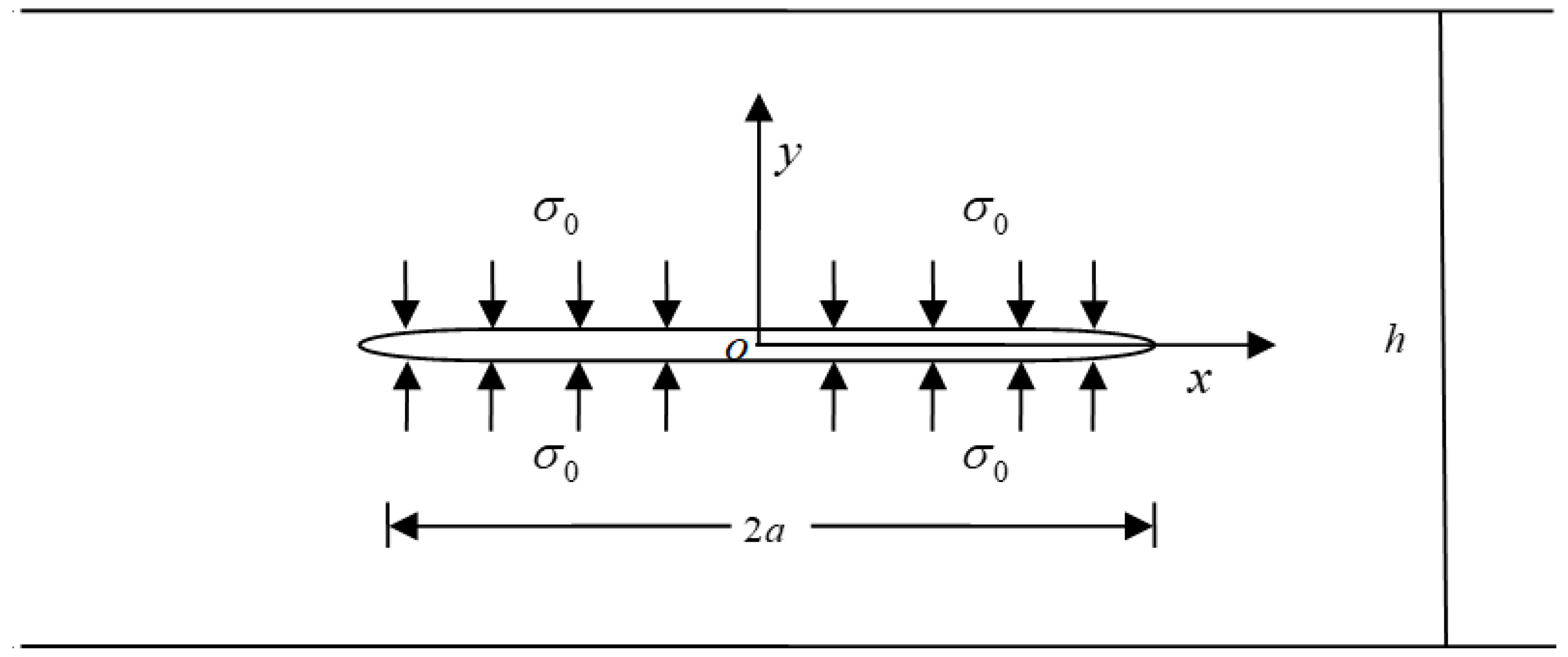
4. Solutions to a Decagonal Quasicrystalline Strip Containing a Centric Crack

It is difficult to determine the solutions to a decagonal quasicrystalline strip containing a crack because of its essential complexity. To avoid this difficulty, we performed a step to determine the conformal mapping from the interior of the unit circle to the exterior of the given crack. Here, we present a new approach for finding the wanted conformal transformation. We constructed a conformal mapping from the physical $z$ plane to the complex $\zeta$ plane, where a conformal map $z=\Phi (\zeta )$ maps the exterior of the crack in the physical $z$ plane to the interior of the unit circle in the $\zeta$ plane.

Figure 2 shows a schematic of a decagonal quasicrystalline strip containing a centric crack. There was a Griffith crack with a length of $2a$ along the $z$ axis embedded at the mid plane of a decagonal quasicrystalline strip with a height of $h$. The surfaces of the crack can be denoted by two coincident lines, namely $y=0^{+}$ and $y=0^{-}$, respectively. The portion $y=0^{\pm }, -a<x<a$ of the crack surfaces were assumed to be subject to the action of uniform loadings ${\sigma }_{yy}=-{\sigma }_0$, $H_{yy}=0$. Meanwhile, we adopted $a$ to simulate the crack length of the strip.

The boundary conditions for this problem can be described as follows:

$$\{\begin{array}{cc}{\sigma }_{yy}={\sigma }_{xy}=0, H_{yy}=H_{yx}=0,& \mathrm{for} y= \pm h,-\infty <x<+\infty ;\\ {\sigma }_{xx}={\sigma }_{xy}=0, H_{xx}=H_{xy}=0,& \mathrm{for} y= \pm 0, -a<x<+a;\\ {\sigma }_{yy}=-{\sigma }_0, {\sigma }_{xy}=0, H_{yy}=H_{yx}=0,& \mathrm{for} y= \pm 0, -a<x<+a.\end{array}$$

(29)

The essential building block in the present application as well as in all of the applications of the method of conformal mappings, is the fundamental mapping $\varphi (\zeta )$ that maps the interior circle onto a Griffith crack with the length of $e^{\raisebox{1ex}{$\pi a$}\!\left/ \!\raisebox{-1ex}{$h$}\right.}-e^{-\raisebox{1ex}{$\pi a$}\!\left/ \!\raisebox{-1ex}{$h$}\right.}$ in the $z_1$ plane:

$$z_1=\varphi (\zeta )=\alpha \left(\zeta +\frac{1}{\zeta }\right) (\alpha =\frac{e^{\raisebox{1ex}{$\pi a$}\!\left/ \!\raisebox{-1ex}{$h$}\right.}-e^{-\raisebox{1ex}{$\pi a$}\!\left/ \!\raisebox{-1ex}{$h$}\right.}}{4})$$

(30)

Second, we introduced some transformations, so that:

$$z_2=z_1+\beta =\varphi (\zeta )+\beta (\beta =\frac{e^{\raisebox{1ex}{$\pi a$}\!\left/ \!\raisebox{-1ex}{$h$}\right.}+e^{-\raisebox{1ex}{$\pi a$}\!\left/ \!\raisebox{-1ex}{$h$}\right.}}{2}), z_3=\ln z_2, z=\frac{h}{\pi }{z}_3$$

(31)

The conformal map was constructed as described in the foregoing section. For the discussion below, we will denote simply $\Phi (\zeta )$ as follows:

$$z=\Phi (\zeta )=\frac{h}{\pi }\ln [\alpha (\zeta +\frac{1}{\zeta })+\beta ]$$

(32)

The point position $\zeta$ in the mathematical domain was mapped by ${\Phi }^{-1}(z)$ onto the point position $z$ in the physical domain. Of course, we could not obtain the solution immediately by means of this transformation. We maintained that Equation (19) holds on and began by writing the unknown functions $h_4(z)$ and $h_3(z)$ by means of the conformal mapping:

$$h_4(\zeta )=h_4(\Phi (\zeta )), h_3(\zeta )=h_3(\Phi (\zeta ))$$

(33)

We can clearly rewrite the boundary condition for the unit circle in the $\zeta$ plane. If we denote $\sigma \equiv e^{i\theta }$ in the unit circle $\gamma$, the boundary conditions can result in:

$$h_4(\sigma )+\overline{h_3(\sigma )}+\frac{\Phi (\sigma )}{\overline{{\Phi }^{\prime }(\sigma )}}\overline{h_4{}^{\prime }(\sigma )}=f_0(\sigma )$$

(34)

Considering that the phason field can be discussed similarly in the above analysis process, we omit the procedure of the phason field here. In the calculation below, we affirmed that the coefficients $B=0$ and $B^{\prime }+i{C}^{\prime }=0$ according to the free stresses at infinity, and meanwhile the circumference of the resultant force was zero:

$$f_0(\sigma )=\frac{i}{32c_1}{\displaystyle \int (T_x+i{T}_y})ds= -\frac{{\sigma }_0}{32c_1}\Phi (\sigma )$$

(35)

where $T_x$ and $T_y$ denote the generalized surface tractions in the $x$-direction and $y$-direction, respectively. Multiplying both sides of Equation (34) and its conjugate equation by $\frac{1}{2\pi i}{\displaystyle {\int }_{\gamma }\frac{1}{\sigma -\zeta }}d\sigma$ and then calculating the Cauchy integration results in:

$$\begin{array}{c}{h}_4(\zeta )+\overline{h_3(0)}+\frac{1}{2\pi i}{\displaystyle {\int }_{\gamma }\frac{\Phi (\sigma )}{\overline{{\Phi }^{\prime }(\sigma )}}\frac{\overline{h_4{}^{\prime }(\sigma )}}{\sigma -\zeta }}d\sigma =\frac{1}{2\pi i}{\displaystyle {\int }_{\gamma }\frac{f_0}{\sigma -\zeta }}d\sigma \\ h_3(\zeta )+\overline{h_4(0)}+\frac{1}{2\pi i}{\displaystyle {\int }_{\gamma }\frac{\overline{\Phi (\sigma )}}{{\Phi }^{\prime }(\sigma )}\frac{h_4{}^{\prime }(\sigma )}{\sigma -\zeta }}d\sigma =\frac{1}{2\pi i}{\displaystyle {\int }_{\gamma }\frac{\overline{f_0}}{\sigma -\zeta }}d\sigma \end{array}\}$$

(36)

where $\sigma$ represents the value of $\zeta$ at the boundary of $\gamma$ in the mapping plane and $h_4(\zeta )={\displaystyle \sum _{k=1}^{\infty }{a}_k}{\zeta }^k$ and $h_3(\zeta )={\displaystyle \sum _{k=1}^{\infty }{b}_k}{\zeta }^k$ are single valued analytic functions in $\left|\zeta \right|<1$. It is necessary to analyze the functions $\frac{\Phi (\sigma )}{\overline{{\Phi }^{\prime }(\sigma )}}\overline{h_4{}^{\prime }(\sigma )}$ and $\frac{\overline{\Phi (\sigma )}}{{\Phi }^{\prime }(\sigma )}{h}_4{}^{\prime }(\sigma )$ in the mathematical domain to compute these integrations. This is the most expensive step in our solution. Using the last two equations together with the conformal map in Equation (32), we obtain:

$$\frac{\Phi (\sigma )}{\overline{{\Phi }^{\prime }(\sigma )}}=-\frac{1}{{\sigma }^2}$$

(37)

$$\frac{\Phi (\sigma )}{\overline{{\Phi }^{\prime }(\sigma )}}\overline{h_4{}^{\prime }(\sigma )}=-\frac{1}{{\sigma }^2}{\displaystyle \sum _{k=1}^{\infty }k\overline{a_k}}\frac{1}{{\sigma }^{k-1}}$$

(38)

$$\frac{\overline{\Phi (\sigma )}}{{\Phi }^{\prime }(\sigma )}{h}_4{}^{\prime }(\sigma )=-{\displaystyle \sum _{k=1}^{\infty }k{a}_k}{\sigma }^{k+1}$$

(39)

It is very easy to prove that Equation (36) can determine the functions $h_4(\zeta )$ and $h_3(\zeta )$ together when these series and function sets of linear equations are posed distinctly. This has been proved with some generality, and the fact can be seen in [10], where the result $h_4{}^{\prime }(\zeta )$, related to the stress intensity factor, is directly given:

$$h_4{}^{\prime }(\zeta )=\frac{{\sigma }_0}{32c_1}\frac{h}{\pi }\left\{\frac{1}{\zeta }+\frac{2\alpha }{1-\beta -2\alpha \zeta }+\frac{\alpha ({\zeta }^2-1)}{\zeta \left[\alpha ({\zeta }^2+1)+\beta \zeta \right]}\right\}$$

(40)

where ${\sigma }_0$ denotes the action of uniform loading, and $c_1, \alpha , \beta$ can be seen in the preceding sections respectively.

When inverse conformal mapping is rarely at hand, it is difficult to calculate the expression of the stress field in terms of the inverse conformal mapping. However, for this problem, if we substitute these expressions into Equation (11), it is very easy to calculate the full stress field for a crack. On the other hand, the stress intensity factor can be seen as the most important quantities, which can be characterized by the universal near-tip fields. Now, we calculate the stress intensity factors from our solution. In fact, the calculation can be completed directly from the solution based on the conformal map as described above. Previous authors derived the following expression for the complex combination (of the real) stress intensity factor [10]:

$$K_{\mathrm{I}}=\frac{\sqrt{\pi }}{16c_1}\underset{\zeta \to 1}{\lim }\frac{h_4{}^{\prime }(\zeta )}{\sqrt{{\omega }^{″}(\zeta )}}={\sigma }_0\sqrt{2h}\frac{2-(e^{\raisebox{1ex}{$\pi a$}\!\left/ \!\raisebox{-1ex}{$h$}\right.}+e^{-\raisebox{1ex}{$\pi a$}\!\left/ \!\raisebox{-1ex}{$h$}\right.})}{1-e^{\raisebox{1ex}{$\pi a$}\!\left/ \!\raisebox{-1ex}{$h$}\right.}}\sqrt{\frac{e^{\raisebox{1ex}{$\pi a$}\!\left/ \!\raisebox{-1ex}{$h$}\right.}}{e^{\raisebox{1ex}{$\pi a$}\!\left/ \!\raisebox{-1ex}{$h$}\right.}-e^{-\raisebox{1ex}{$\pi a$}\!\left/ \!\raisebox{-1ex}{$h$}\right.}}}$$

(41)

This result can be extended to mode $\mathrm{II}$ of decagonal quasicrystals. Due to its similarity, the process was omitted. In particular, this special result (Equation (41)) can be converted into the results obtained in [10]. If we let $\frac{a}{h}\to 0$ or $h\to \infty$, the expression (Equation (41)) can be converted into:

$$K_{\mathrm{I}}={\sigma }_0\sqrt{\pi a}$$

(42)

which is the stress intensity factor of the decagonal point group 10 mm quasicrystals of the infinite plate weakened by a Griffith crack [10].

5. Conclusions and Discussion

Defects occupy a very important role in the study of the mechanical behavior of materials. Of course, it is very difficult to solve defects, including notch and crack, due to the complicated configuration. By introducing conformal mapping, we analyzed the strict theory of the complex potential method for the plane problems of two-dimensional quasicrystals. These results not only developed the methodology of the complex analysis of quasicrystal elasticity, but are also significant for the fracture analysis of the material. Meanwhile, the results given in this paper are exact analytical expressions, which provide a useful theoretical basis for the plane problems of decagonal quasicrystals. The application of the complex potential method displayed success in solving these problems. These results can be exactly reduced into the well-known classical solution in conventional structural materials.

References

- Shechtman, D.; Blech, I.; Gratias, D.; Cahn, J.W. Metallic phase with long-range orientational order and no translational symmetry. Phys. Rev. Lett. 1984, 53, 1951–1953. [Google Scholar]
- Bak, P. Phenomenological theory of icosahedral in commensurate (quasiperiodic) order in Mn-Al alloys. Phys. Rev. Lett. 1985, 54, 1517–1519. [Google Scholar]
- Socolar, J.E.S.; Lubensky, T.C.; Steinhardt, P.J. Phonons, phasons and dislocations in quasicrystals. Phys. Rev. B 1986, 34, 3345–3360. [Google Scholar]
- Edagawa, K. Phonon-phason coupling in decagonal quasicrystals. Philos. Mag. 2007, 87, 2789–2798. [Google Scholar]
- Cheminkov, M.A.; Ott, H.R.; Bianchi, A.; Migliori, A.; Darling, T.W. Elastic moduli of a single quasicrystal of decagonal Al-Ni-Co: Evidence for transverse elastic isotropy. Phys. Rev. Lett. 1998, 80, 321–324. [Google Scholar]
- Tanaka, K.; Mitarai, Y.; Koiwa, M. Elastic constants of Al-based icosahedral quasicrystals. Philos. Mag. A 1996, 73, 1715–1723. [Google Scholar]
- Ding, D.H.; Yang, W.G.; Hu, C.Z. Generalized elasticity theory of quasicrystals. Phys. Rev. B 1993, 48, 7003–7010. [Google Scholar]
- Hu, C.Z.; Wang, R.H.; Ding, D.H. Symmetry groups, physical property tensors, elasticity and dislocations in quasicrystals. Rep. Prog. Phys. 2000, 63, 1–39. [Google Scholar]
- Jeong, H.C.; Steinhardt, P.J. Finite-temperature elasticity phase transition in decagonal quasicrystals. Phys. Rev. B 1993, 48, 9394–9403. [Google Scholar] [Green Version]
- Fan, T.Y. Mathematical Theory of Elasticity of Quasicrystals and Its Applications; Springer: Heideberg, Germany, 2010. [Google Scholar]
- Radi, E.; Mariano, P.M. Stationary straight cracks in quasicrystals. Int. J. Fract. 2010, 166, 102–120. [Google Scholar]
- Radi, E.; Mariano, P.M. Steady-state propagation of dislocations in quasi-crystals. Proc. R. Soc. A Math. Phys. 2011, 467, 3490–3508. [Google Scholar] [Green Version]
- Mariano, P.M.; Planas, J. Phason self-actions in quasicrystals. Physica D 2013, 249, 24946–24957. [Google Scholar]
- Wang, J.B.; Mancini, L.; Wang, R.H.; Gastaldi, J. Phonon- and phason-type spherical inclusions in icosahedral quasicrystals. J. Phys. Condens. Matter 2003, 15, L363–L370. [Google Scholar]
- Li, X.F.; Duan, X.Y.; Fan, T.Y. Elastic field for a straight dislocation in a decagonal quasicrystal. J. Phys. Condens. Matter 1999, 11, 703–711. [Google Scholar]
- Li, X.F.; Fan, T.Y.; Sun, Y.F. A decagonal quasicrystal with a Griffith crack. Philos. Mag. A 1999, 79, 1943–1952. [Google Scholar]
- Gao, Y.; Ricoeur, A. The refined theory of one-dimensional quasi-crystals in thick plate structures. J. Appl. Mech. 2011, 78, 031021. [Google Scholar]
- Li, L.H.; Fan, T.Y. Complex function method for solving notch problem of point 10 two-dimensional quasicrystal based on the stress potential function. J. Phys. Condens. Matter 2006, 18, 10631–10641. [Google Scholar]
- Li, X.Y. Fundamental solutions of penny-shaped and half infinite plane cracks embedded in an infinite space of one dimensional hexagonal quasi-crystal under thermal loading. Proc. R. Soc. A Math. Phys. 2013, 469, 20130023. [Google Scholar]
- Li, X.Y. Elastic field in an infinite medium of one-dimensional hexagonal quasicrystal with a planar crack. Int. J. Solids Struct. 2014, 51, 1442–1455. [Google Scholar] [Green Version]
- Wollgarten, M.; Beyss, M.; Urban, K.; Liebertz, H.; Koster, U. Direct evidence for plastic deformation of quasicrystals by means of a dislocationmechanism. Phys. Rev. Lett. 1993, 71, 549–552. [Google Scholar]
- Feuerbacher, M.; Bartsch, M.; Grushko, B.; Messerschmidt, U.; Urban, K. Plastic deformation of decagonal Al-Ni-Co quasicrystals. Philos. Mag. Lett. 1997, 76, 369–376. [Google Scholar] [Green Version]
- Messerschmidt, U.; Bartsch, M.; Feuerbacher, M.; Geyer, B.; Urban, K. Friction mechanism of dislocation motion in icosahedralAl-Pd-Mn quasicrystals. Philos. Mag. A 1999, 79, 2123–2135. [Google Scholar]
- Schall, P.; Feuerbacher, M.; Bartsch, M.; Messerschmidt, U.; Urban, K. Dislocation density evolution upon plastic deformation of Al-Pd-Mn single quasicrystals. Philos. Mag. Lett. 1999, 79, 785–796. [Google Scholar]
- Geyer, B.; Bartsch, M.; Feuerbacher, M.; Urban, K.; Messerschmidt, U. Plastic deformation of icosahedral Al-Pd-Mn single quasicrystals I. Experimental results. Philos. Mag. A 2000, 80, 1151–1163. [Google Scholar]
- Rosenfeld, R.; Feuerbacher, M. Study of plastically deformed icosahedral Al-Pd-Mn single quasicrystals by transmission electron microscopy. Philos. Mag. Lett. 1995, 72, 375–784. [Google Scholar]
- Caillard, D.; Vanderschaeve, G.; Bresson, L.; Gratias, D. Transmission electron microscopy study of dislocations and extended defects in as-grown icosahedral Al-Pd-Mn single grains. Philos. Mag. A 2000, 80, 237–253. [Google Scholar]
- Muskhelishvili, N.I. Some Basic Problems of Mathematical Theory of Elasticity; Noordhoff: Groningen, The Netherlands, 1963. [Google Scholar]
Figure 1.
A schematic figure for an elliptic notch.
Figure 2.
A decagonal quasicrystalline strip with a centric crack.
© 2019 by the authors. Licensee MDPI, Basel, Switzerland. This article is an open access article distributed under the terms and conditions of the Creative Commons Attribution (CC BY) license (http://creativecommons.org/licenses/by/4.0/).
Share and Cite
MDPI and ACS Style
Cao, H.; Shi, Y.; Li, W. Analytic Solutions to Two-Dimensional Decagonal Quasicrystals with Defects Using Complex Potential Theory. Crystals 2019, 9, 209. https://0-doi-org.brum.beds.ac.uk/10.3390/cryst9040209
AMA Style
Cao H, Shi Y, Li W. Analytic Solutions to Two-Dimensional Decagonal Quasicrystals with Defects Using Complex Potential Theory. Crystals. 2019; 9(4):209. https://0-doi-org.brum.beds.ac.uk/10.3390/cryst9040209
Chicago/Turabian StyleCao, Haobai, Yiqing Shi, and Wu Li. 2019. "Analytic Solutions to Two-Dimensional Decagonal Quasicrystals with Defects Using Complex Potential Theory" Crystals 9, no. 4: 209. https://0-doi-org.brum.beds.ac.uk/10.3390/cryst9040209
Note that from the first issue of 2016, this journal uses article numbers instead of page numbers. See further details here.