Compound Extremes in Hydroclimatology: A Review

1
Green Development Institute, College of Water Sciences, Beijing Normal University, Beijing 100875, China
2
Department of Biological and Agricultural Engineering and Zachry Department of Civil Engineering, Texas A&M University, College Station, TX 77843-2117, USA
*
Author to whom correspondence should be addressed.
Water 2018, 10(6), 718; https://0-doi-org.brum.beds.ac.uk/10.3390/w10060718
Submission received: 24 April 2018
/
Revised: 28 May 2018
/
Accepted: 30 May 2018
/
Published: 1 June 2018
(This article belongs to the Special Issue Climate Variability and Climate Change Impacts on Land Surface, Hydrological Processes and Water Management)
Abstract
:Extreme events, such as drought, heat wave, cold wave, flood, and extreme rainfall, have received increasing attention in recent decades due to their wide impacts on society and ecosystems. Meanwhile, the compound extremes (i.e., the simultaneous or sequential occurrence of multiple extremes at single or multiple locations) may exert even larger impacts on society or the environment. Thus, the past decade has witnessed an increasing interest in compound extremes. In this study, we review different approaches for the statistical characterization and modeling of compound extremes in hydroclimatology, including the empirical approach, multivariate distribution, the indicator approach, quantile regression, and the Markov Chain model. The limitation in the data availability to represent extremes and lack of flexibility in modeling asymmetric/tail dependences of multiple variables/events are among the challenges in the statistical characterization and modeling of compound extremes. Major future research endeavors include probing compound extremes through both observations with improved data availability (and statistical model development) and model simulations with improved representation of the physical processes to mitigate the impacts of compound extremes.
1. Introduction
The climate system has been changing significantly as exhibited by global warning, which is expected to intensify (and accelerate) the hydrologic cycle due to the involvement of certain temperature dependence processes. This would lead to changes in the duration, frequency, spatial extent, and timing of extreme weather and climate events [1,2,3]. A variety of climate and weather related extremes, such as droughts, floods, heavy rainfalls, heat waves, tornadoes, cyclones or storms, have been shown to change significantly in the past, posing serious challenges to different sectors of the society including water, energy and food and their nexus (i.e., the water-energy-food nexus (WEF)) [4,5,6,7,8,9,10]. Moreover, recent studies based on climate projections have revealed a potential increase in these extremes in the future [3,11,12,13,14,15], which calls for an improved understanding of the changes in extremes and their impacts under global warming.
Traditionally, studies on weather and climate extremes have mostly focused on the extremes from a single process or variable, such as heavy precipitation or maximum temperature. For example, a multitude of studies have shown increases in the severity, duration, and frequency of precipitation and temperature extremes [4,16,17,18,19,20,21]. The extreme value theory (EVT) constitutes the basis for statistical modeling of univariate extremes in this regard, which can generally be achieved with the probability distribution of individual extremes, such as generalized extreme value (GEV) distribution or generalized Pareto distribution (GPD) based on the annual maxima or peak over threshold [22,23]. However, hydroclimatic variables are interconnected and thus focusing on a single variable or extreme may not be sufficient to comprehensively characterize the impact of extremes, which calls for multivariate modeling techniques.
Compound extremes, which are also referred to as simultaneous, concurrent, or coincident extremes (e.g., the concurrence or succession of multiple extremes/events), may exacerbate an adverse impact, leading to larger impacts to human society and the environment than those from individual extremes alone [24,25,26]. The past decade has witnessed an upsurge in studies of compound extremes, such as drought and heat wave (or low precipitation and high temperature) at different regions including Europe (2003 and 2015), Russia (2010), and California in the U.S. (2014) [4,27,28,29,30,31]. For example, the recent 2012 extreme drought in the central U.S. with record deficit in precipitation was accompanied by high temperatures during the May–August growing season, which significantly affected crop yields [32].
The physical mechanism of a compound extreme (e.g., compound flood) is rather complex depending on a variety of weather and hydrological processes [24,25,33,34,35]. Studies based on both models and observations have been devoted to the modeling of multiple drivers or processes of compound extremes. Correlations between occurrences of extremes may be induced due to a common external factor (e.g., regional warming), mutual reinforcement of two events (e.g., land surface feedback) or conditional dependence of the occurrence of one event to another event (e.g., extreme precipitation and soil moisture for flood) in the weather or hydroclimatic system [25,36]. Statistical methods have been commonly employed to model the correlation or interaction of multiple variables or processes that may lead to compound extremes. One example is the occurrence of drought and extreme heat in summer, which may be largely due to the land atmosphere feedback. Studies have shown that the number of occurrences of the compound drought and extreme heat increased in different regions [29,37]. In addition, the quantile regression method has been widely used for the assessments of the contribution of the antecedent soil moisture deficit on the occurrence of high temperature [38,39], leading to a compounded dry and hot extreme. In addition, coastal flooding may be caused by large waves combined with a high sea level and its multivariate distribution has been employed to study the compound extreme of wave height and water level at different coastline stretches around the globe [40,41,42,43,44,45,46]. These studies advanced our understanding of compound extremes and how to enhance the capacity to cope with the adverse impacts of these climate anomalies. However, a thorough introduction and comparison of statistical methods for assessing compound extremes is lacking.
The aim of this study therefore is to review commonly used statistical methods for the characterization and modeling of compound extremes in hydroclimatology. This paper is organized as follows. The definition and types of compound extremes are introduced in Section 2. An introduction of statistical modeling of compound extremes is provided in Section 3. Section 4 discusses several topics related to compound extremes, followed by conclusions in Section 5.
2. Compound Extremes
2.1. Definition of Compound Extremes
There are different definitions of compound extremes/events. The IPCC Special Report on Managing the Risks of Extreme Events and Disasters to Advance Climate Change Adaptation (IPCC SREX) defines the compound event as follows [25]:
“(1) two or more extreme events occurring simultaneously or successively, (2) combinations of extreme events with underlying conditions that amplify the impact of the events, or (3) combinations of events that are not themselves extremes but lead to an extreme event or impact when combined.”
It is emphasized in this definition that the coincidence of several factors, each of which may not necessary to be extreme, may lead to adverse and extreme impacts [47,48]. By categorizing compound extremes into different classes, this definition is crucial in understanding the phenomenon; however, some events are hard to be classified under this definition [24]. Recently, another definition of compound event has been given as follows [24]:
“A compound event is an extreme impact that depends on multiple statistically dependent variables or events.”
This definition of compound extremes/events emphasizes three aspects, including the impact, presence of multiple variables (or events), and statistical dependence. A common feature of the two definitions is that the compound extreme generally involves the interaction (or dependence) of multiple drivers (or variables/events), either of the same type (e.g., extreme rainfall at both upstream and downstream) or different types (e.g., compound drought and hot extreme). This highlights that the dependence modeling of multivariate random variables plays a central role in the statistical modeling of compound extremes.
2.2. Typical Compound Extremes
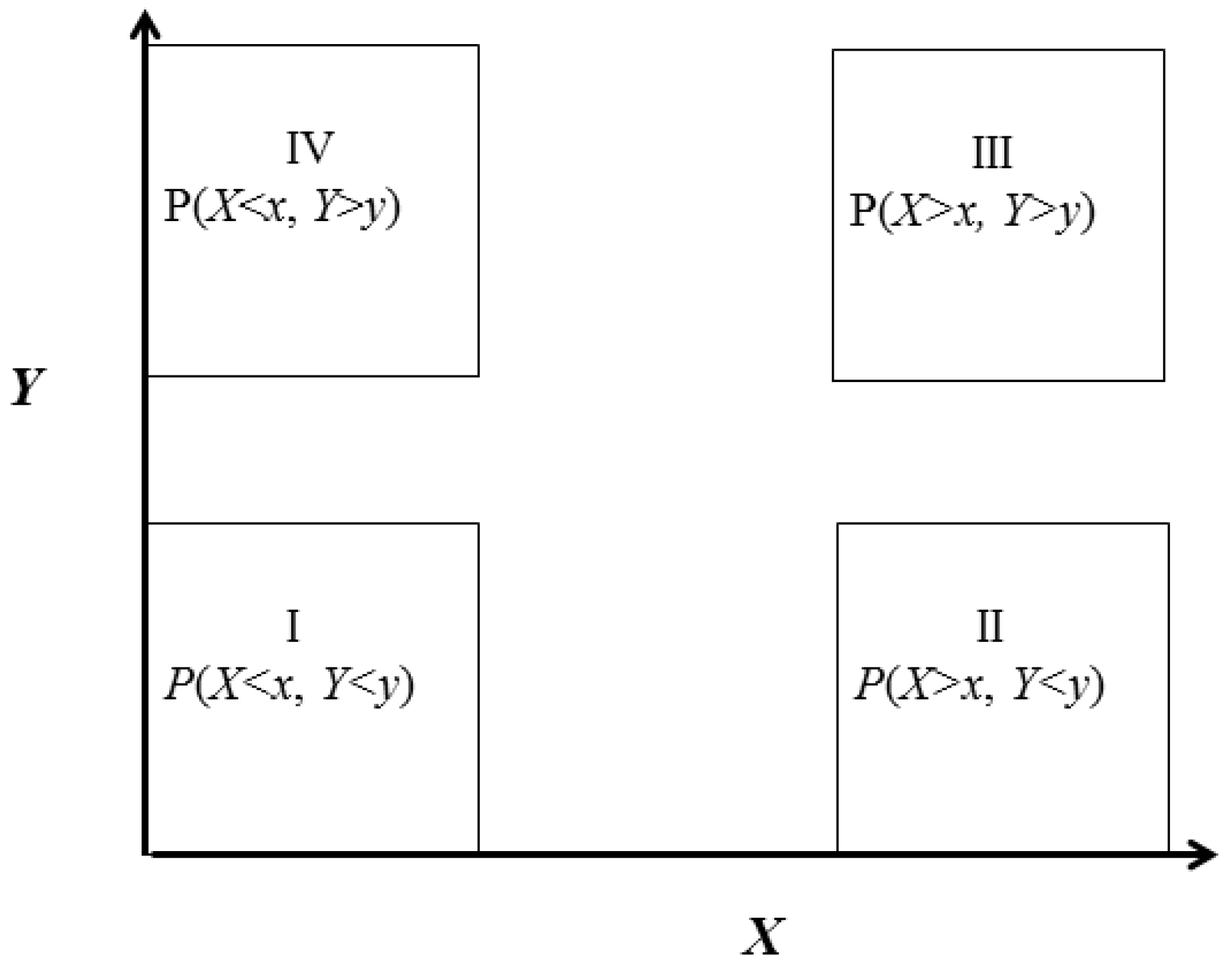
The compound extremes refer to a variety of cases in hydrology and climatology. In this study, compound extremes in the bivariate case are classified into different types in which four regions of extremes (I, II, III, and IV) are defined, as illustrated in Figure 1. A summary of typical compound extremes is provided in the Appendix A, such as the drought and hot extreme, precipitation and temperature extreme, and compound flood. Note that there are other types of compound events that may be of particular interest, such as the combined wind speed and storm surges (or precipitation) [36,49,50], combined humidity and temperature extremes [51], and the co-occurrence of particulate matter (PM2.5) and maximum temperature [52].
The compound nonexceedance- nonexceedance extremes are illustrated in region I, in which both variables lower than certain quantiles are of primary interest, such as the deficit in both precipitation and soil moisture. Drought, a typical example in this case, is commonly classified as meteorological, hydrological, agricultural, or socioeconomic drought [53], which may occur separately or simultaneously. Recently, substantial efforts have been devoted to the drought characterization from a multivariate perspective based on the concurrent deficit of multiple variables [54]. The compound exceedance- exceedance extremes type falls in Region III, in which two variables higher than certain values are of primary interest, such as storm surges (or sea level) and high precipitation (river discharge) [35,48,55,56,57,58,59,60]. For example, in coastal areas, the risk of flood will increase if high coastal water level (or storm surge) occurs simultaneously with high precipitation/runoff, leading to the increase of the river water level [55,56,61,62]. In addition, the combination of high temperature and heavy precipitation in the spring season in certain regions (e.g., Norway) can result in flooding when runoff from snow-melt adds to river discharge due to rainfall [47].
Regions II and IV indicate the compound exceedance- nonexceedance extremes, in which one variable lower (or higher) than a threshold with the other variable higher (or lower) than a threshold is of primary interest. Drought and heatwave have been among the most commonly investigated compound extremes of this type [27,37,63,64,65], which may promote wildfires [66], affect agricultural production [67,68], or reduce the net primary productivity (NPP) [69,70]. Drought and hot extremes are interconnected, which is mostly due to the positive feedback in transitional regions between a wet and dry climate, in that drought condition may be amplified/exacerbated when accompanied by heat wave, while drought may create favorable conditions for hot extreme or heat wave [4,8,13,38,71,72].
Apart from multiple extremes at the same time introduced above, the compound extreme also refers to sequential (or temporal clustering, successive) extremes, such as the temporal clustering of extreme sea level and skew surge events [73]. The compound extremes at different locations (or spatial extremes) may also be of interest, such as simultaneous flood in a wide area or extreme precipitation at multiple stations [74,75,76]. Understanding these properties of the compound extreme is important for the characterization and modeling to facilitate mitigation measures to reduce its impacts.
3. Statistical Approaches
Both models and observations have been used to explore the relationship between multiple variables/components of compound extremes. Due to limited observations of extremes (or rare events), the statistical inference of compound extremes and the extrapolation beyond observations are of particular interest. In the following, we mainly focus on methods for modeling compound extremes from a statistical perspective. These methods include the empirical approach, multivariate distribution, the indicator approach, quantile regression, and the Markov Chain model.
3.1. Empirical Approach
The empirical approach for the analysis of compound extremes is executed through counting the number of concurrent or consecutive occurrences of multiple extremes [29,51,57,77,78,79,80]. This approach mainly characterizes the occurrence or variability of compound extremes. The individual extreme is first defined (e.g., based on a threshold or percentile) [81], which is then used to obtain the quantity of compound extremes based on the co-occurrence of individual extremes. For example, a wide variety of indices of daily precipitation and temperature extremes (e.g., warm days defined as percentage of time when daily max temperature >90th percentile) have been developed by the joint CCI/CLIVAR/JCOMM Expert Team on Climate Change Detection and Indices (ETCCDI) (available at: http://cccma.seos.uvic.ca/ETCCDI/list_27_indices.html), which are also known as the ‘ETCCDI’ indices [82,83,84,85]. Accordingly, a multitude of compound extremes can be defined by counting the concurrence of these individual extremes. Usually the number of compound extremes for each period (i.e., month, year) is first computed and statistical analysis (e.g., trend analysis, change point analysis) is employed to detect associated changes.
The compound precipitation and temperature extreme has been widely explored. The precipitation (and temperature) extreme for a specific period can be defined as dry/wet (and cold/warm) when precipitation (and temperature) is lower/higher than certain thresholds (e.g., 25th/75th percentile). The associated four compound extremes (dry-warm, dry-cold, wet-warm, wet-cold) can then be defined when the two extremes occur concurrently [29,77,80]. The assessment of changes of these four compound extremes generally showed an increase in the warm mode of compound extremes (i.e., dry-warm, wet-warm). For example, it has been found that the occurrence of warm/dry and warm/wet modes in Europe have increased in the 20th century and will continue to increase in the 21th century [77]. In addition, assessments of combined precipitation and temperature modes in Spanish mountains revealed an increase in the frequency of dry-warm and wet-warm days [80].
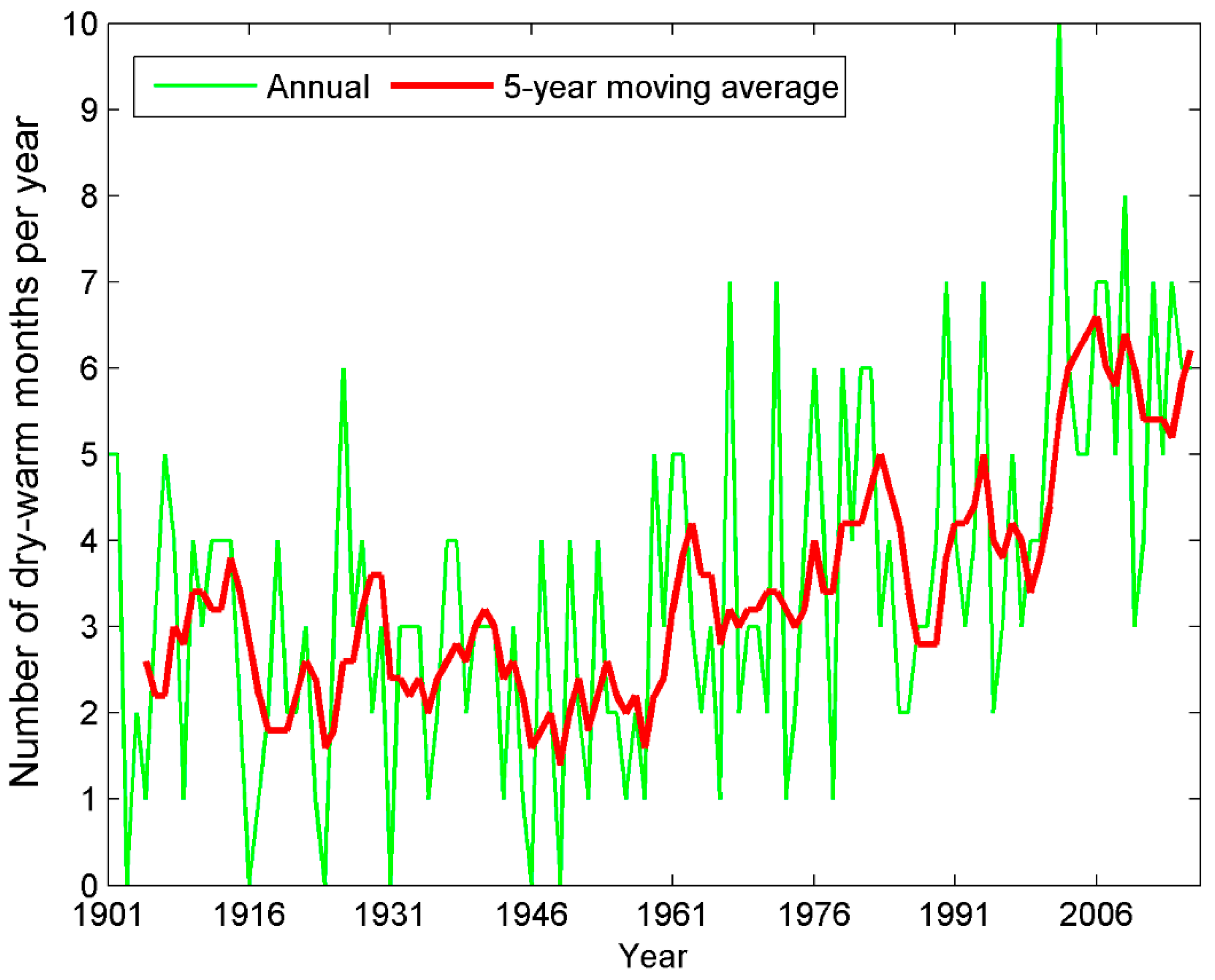
We use the monthly precipitation and temperature data near Melbourne, Australia (Longitude: 144.9, Latitude: −37.8) to illustrate this approach. The monthly data for the period 1901–2016 were obtained from the Climatic Research Unit (CRU TS3.25) (using the nearest grid). Note that the gridded data should be used with caution in analyzing extreme events due to the reason that extremes may be smoothed during the interpolation process [86,87,88,89]. We use these data here and in the following sections mainly for illustrative purposes. Based on the definition above, we computed the number of compound dry-warm extreme occurrences for each year (and 5-year running average) during 1901–2016 for Melbourne, Australia, as shown in Figure 2. A significant increase in the occurrence of the dry-warm extreme is shown during the past century, implying the increased risk of a compound extreme under global warming in this region [90].
3.2. Multivariate Distribution
A key property of the compound extreme is that dependence between different contributing variables (or drivers) generally exists. The multivariate distribution plays a critical role in modeling dependence of multiple variables/extremes for a variety of applications (e.g., estimate the combined risk of extremes) [49,91]. For example, the multivariate distribution has been used to explore joint properties of precipitation and temperature (or their extremes) for frequency assessments or statistical simulations [92,93,94,95,96,97]. There are many ways to construct the multivariate distribution, such as parametric distribution, copula, entropy, and nonparametric models [98]. Copula is among the most recent advances in multivariate dependence modeling for a variety of applications in hydrology and climatology [99,100,101,102,103,104,105,106,107,108,109,110,111,112]. It enables the construction of the joint distribution in a flexible way in which the marginal distribution is independent of the modeling of dependence structure. In the following, we introduce the copula model for constructing the multivariate distribution to model compound extremes.
3.2.1. Copula Approach
For two random variables X and Y with marginal distributions U and V, respectively, the joint distribution can be expressed with a copula C as [113]:
where θ is the parameter of the copula.
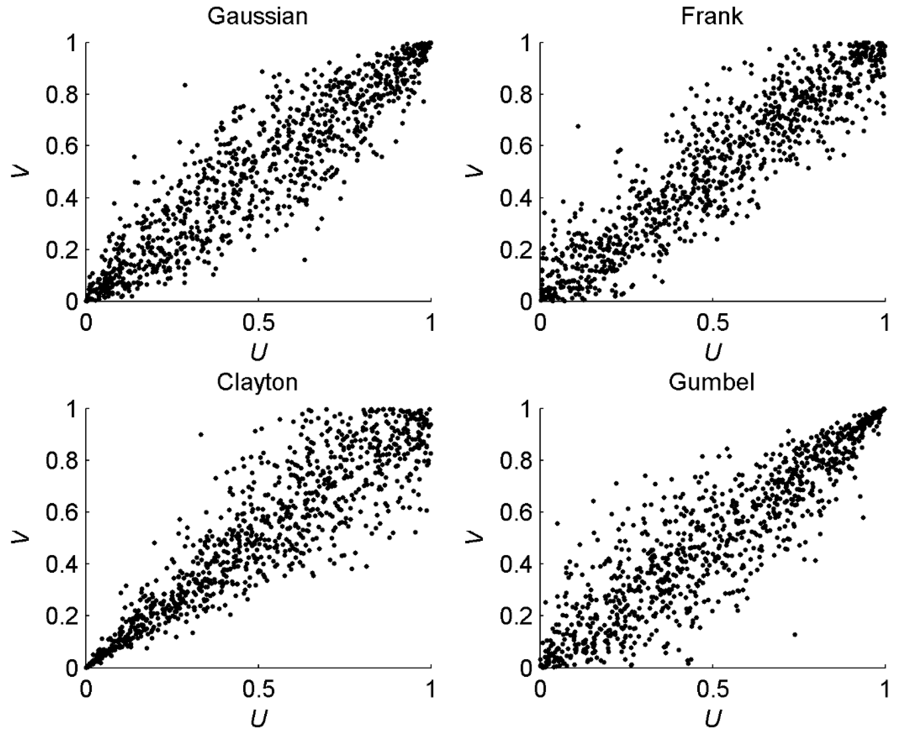
Several copula families, including elliptical (e.g., Gaussian, Student t), Archimedean (e.g., Frank, Clayton, Gumbel), and extreme-value copula (Gumbel, Galambos, extremal-t, and Hüsler–Reiss), have been commonly used for the construction of multivariate distributions, which show different properties in dependence modeling. Four commonly used 2-parameter copulas are shown in Table 1. Random samples with a sample size of 1000 from these four copulas are illustrated in Figure 3 to show the different properties of these copulas in modeling multivariate variables. Variables drawn from the Gaussian and Frank copula exhibit symmetric dependences. The difference is that the dependence in the Frank copula is weaker in tails and stronger in the center of the distribution compared with the Gaussian copula [114]. Both the Clayton and Gumbel copula exhibit asymmetric dependences. Specifically, the Clayton copula exhibits the lower tail dependence (LTD) while the Gumbel copula shows the upper tail dependence (UTD) [115]. These properties imply that the Clayton copula is best suited for applications with two outcomes likely experiencing low values together while the Gumbel copula is suitable when two outcomes are likely to realize upper tail values simultaneously [114]. The extreme-value copula is commonly used for modeling the dependence structure between a rare event and the Gumbel copula is the only copula that is both an extreme value copula and an Archimedean copula [116,117,118,119].
3.2.2. Joint Probability
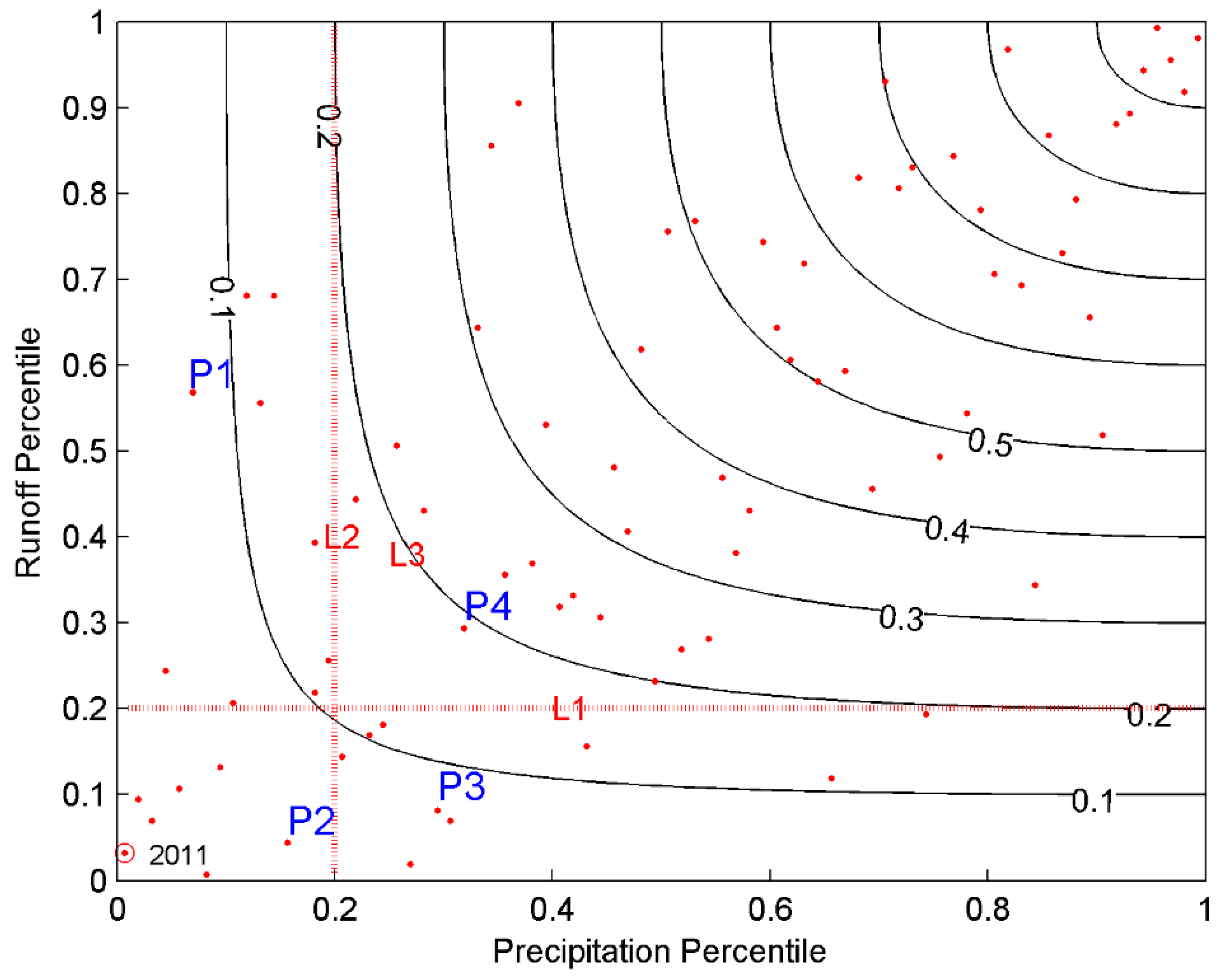
The multivariate distribution can be employed to model the joint behavior of compound extremes and enables the comparison of individual and compound extremes based on the marginal probability and joint probability (or percentile). We use the compound meteorological and hydrological drought as an example to illustrate the comparison, which may be applied to other compound extremes (e.g., drought and heatwave, storm surge and rainfall). Based on the monthly precipitation and runoff for the period 1932–2011 from climate division 2 in Texas, USA (obtained from the National Climatic Data Center, National Oceanic and Atmospheric Administration), the percentile of precipitation and runoff (6-month time scale) in July is constructed with the Gumbel copula. The 20th percentile is specified as the threshold to define the drought condition, which is shown in Figure 4 (i.e., lines L1 and L2). The 20th percentile of the joint distribution is also specified as a threshold to measure the compound extreme and the joint percentile is shown in Figure 4 (L3 represents the 20th joint percentile). The upper left region (e.g., P1(0.07, 0.58)) or the lower right region (e.g., P3(0.29,0.10)) is the case with the occurrence of only meteorological drought or hydrological drought. The lower left region (e.g., P2(0.16,0.07)) is the case with the concurrence of both meteorological and agricultural drought (i.e., compound drought). Of particular interest is the marked region bounded by L1, L2 and L3 (e.g., P4(0.32,0.32)), in which neither the meteorological drought nor the hydrological drought occurs. It can be seen that the joint percentile of this region is lower than the 20th percentile, which indicates the occurrence of the compound meteorological and hydrological drought. This highlights that the compound extreme may occur even when neither of its components are extreme.
The multivariate distribution has been applied for the frequency analysis of compound extremes by computing the return period. An important way to quantify the risk of extremes is through a frequency analysis of individual extremes entailing a return period (or return level) [120,121]. Usually this return period can be obtained from the probability P with the relationship T = μ/(1 − P), where μ is the mean interval time and P is the nonexceedance (or nonexceedance) probability of interest [122]. For univariate extremes, efforts are needed in selecting the distribution of extremes either through block maxima or threshold exceedance. In addition, other approaches such as the fractal approach (or power law distribution) have also been discussed for the frequency analysis of rare events in hydrology [123,124,125]. In the multivariate case, there are different ways to estimate the return period of multiple variables or extremes either based on the joint distribution or the Kendall distribution function [122,126,127,128,129,130,131,132]. Traditionally, the commonly used method in the bivariate case refers to the estimation of the joint probability P(X ≤ x and Y ≤ y), P(X ≤ x and Y > y) and P(X > x and Y > y), which can be applied for different cases of the compound extremes in the Appendix A. For example, P(X ≤ x and Y ≤ y) is of interest for the compound meteorological-agricultural drought while P(X ≤ x and Y > y) is of interest for the compound drought-hot extremes.
We use the compound meteorological and agricultural drought to illustrate the application based on the monthly precipitation and runoff for the period 1932–2011 from climate division 2 in Texas, USA. The Standardized Precipitation Index (SPI) [133] and Standardized Runoff Index (SRI) [134] are commonly used drought indicators to track the meteorological drought and hydrological drought and are used in this study. For the computation of these indices, the empirical Gringorten plotting position formula is used to estimate the marginal probability of precipitation and runoff (6-month time scale) [135]. The joint return period of the SPI and SRI can be used for the frequency analysis of compound meteorological and agricultural drought. The empirical return period of the individual meteorological drought and hydrological drought in 2011 is 143 and 32 years, respectively. Based on joint probability, the joint return period of the compound meteorological-hydrological drought is 396 years. These results imply that the drought event in 2011 in this climate division is a 396-year event if both the meteorological and agricultural drought are taken into account. These results are consistent with previous studies, which highlighted that the risk of the compound extreme may be underestimated if the dependence between contributing variables was ignored [48,61,136].
3.2.3. Conditional Probability
The multivariate distribution approach also enables the quantification of the conditional relationship between two or more extremes. For example, the conditional distribution of the maximum temperature given antecedent meteorological drought can be used to quantify the impact of drought on hot extremes, which reflects the land surface feedback that contributes to the compound drought and hot extremes [38,137,138]. Existing approaches for multivariate extreme modeling are generally applicable to the case in which all variables are simultaneously extreme. As stated before, compound extremes may occur when not all variables need to be extreme. In this case, the conditional extreme model [139,140] is an attracting choice since it enables the dependence modeling of a multivariate extreme in which only part of the component is extreme [141,142].
Two types of conditional distributions are of primary interest in studying compound extremes, either conditioned on a specific value (e.g., u = u0) or range (e.g., u < u0). The conditional probability of V ≤ v given U = u0 can be expressed with a copula C as [143]:
Based on Equations (2) and (3), the conditional probability and return period can be derived accordingly [143,144].
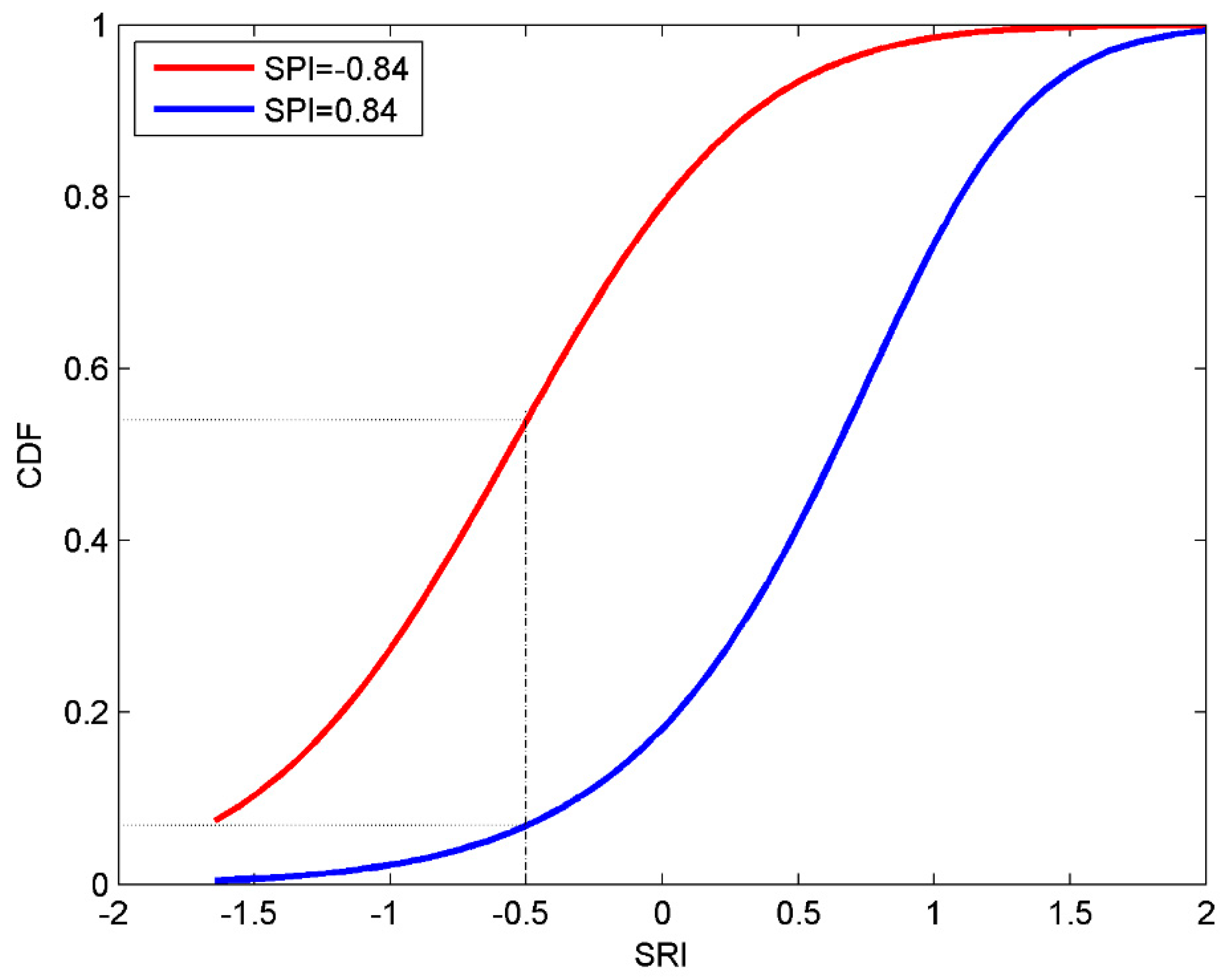
We use two examples to illustrate the application of the conditional distribution in a compound extreme analysis. Based on the SPI and SRI of Climate Division 2 in Texas, the conditional distribution of the hydrological drought (SRI) given meteorological drought (SPI) (SPI = −0.84 and 0.84) can be modeled with the Gumbel copula, which is shown in Figure 5. It can be seen that given the meteorological drought (SPI = −0.84) in the antecedent period, the probability of SRI lower than −0.5 is higher than that given the wet condition (SPI = 0.84). As another example, based on monthly precipitation and daily maximum temperature for the station at Dallas Fort Worth, TX for the period 1948–2010 obtained from the Global Historical Climatology Network (GHCN) version 2 (https://www.ncdc.noaa.gov/ghcnm/v2.php), the conditional distribution of maximum temperature given antecedent meteorological drought can be constructed to quantify the impact of drought on hot extremes. For the SPI of July and daily maximum temperature of August (with Pearson correlation −0.33), the joint distribution is constructed using the Frank copula for illustration purposes. The conditional probability of hot extremes higher than the 80th percentile conditioned on the SPI (SPI ≤ −0.84 and SPI > 0.84) in the antecedent period is computed as 0.40 and 0.06, implying the impact of an antecedent drought on the subsequent hot extremes (i.e., drought induced high temperature). The univariate return period of hot extremes higher than the 80th percentile is 5 years, which is longer than the conditional return period given SPI ≤ −0.84 (2.5 years). These results indicate that ignoring the dependences between contributing variables of compound extreme may lead to an underestimation of risk.
3.3. Indicator Approach
Different indicators have been defined for the extremes in the univariate case [82,145]. The difference between univariate extremes and compound extremes is that in the multivariate setting, there is no natural order of extremes (or variables) in higher dimensions. As such, a “threshold” that can be used to define extremes in the multivariate setting does not exist [126]. For the indicator approach, information from multiple variables or spatiotemporal fields can be distilled into an indicator (by integrating multiple measures of extremes into one index) to inform users the condition and variability of extremes in a specific area [7]. To summarize, an indicator I can be defined to study compound extremes of multiple variables X, Y, …, Z as follows:
where the function G can be any form (e.g., a linear combination, maximum, joint distribution) that serves to project the multiple variable into a unique index I. Based on the indicator I, the compound extremes can be characterized flexibly in different aspects including duration, severity, intensity, and spatial extent.
In the compound extreme analysis, the Climate Extremes Index (CEI) [146,147,148] is such an index defined as the average (or linear combination) of multiple indicators of extremes (including drought, and extremes of precipitation and temperature) in the U.S. [148]. The multiple variables or extremes can also be combined based on the “structure variable”, such as Z = max (Mx, My), where Mx and My are two extremes (e.g., combined thunderstorm and tornado) [149,150,151,152]. Among different ways of developing indicators, the multivariate distribution has been commonly explored for characterizing compound extremes from a multivariate perspective, since it completely describes the joint behavior of two or more variables [54,60,153]. The joint probability or percentile P1 = P(X ≤ x, Y ≤ y) can be employed as the measure of the compound extreme of both variable X and Y lower than certain thresholds (e.g., 10th percentile). Similarly, the joint probability P2 = P(X ≤ x, Y > y) can be used as a measure of the compound extreme with X lower than a specific threshold (e.g., 10th percentile) and Y exceeding a higher threshold (e.g., 90th percentile), such as the compound drought and hot extremes.
As an example, the Multivariate Standardized Drought Index (MSDI) can be defined to characterize the compound meteorological and hydrological drought based on the joint probability of SPI and SRI, which can be expressed as [135]:
where Φ is the standard normal distribution. Here the joint distribution is estimated with the empirical Gringorten distribution in the bivariate case.
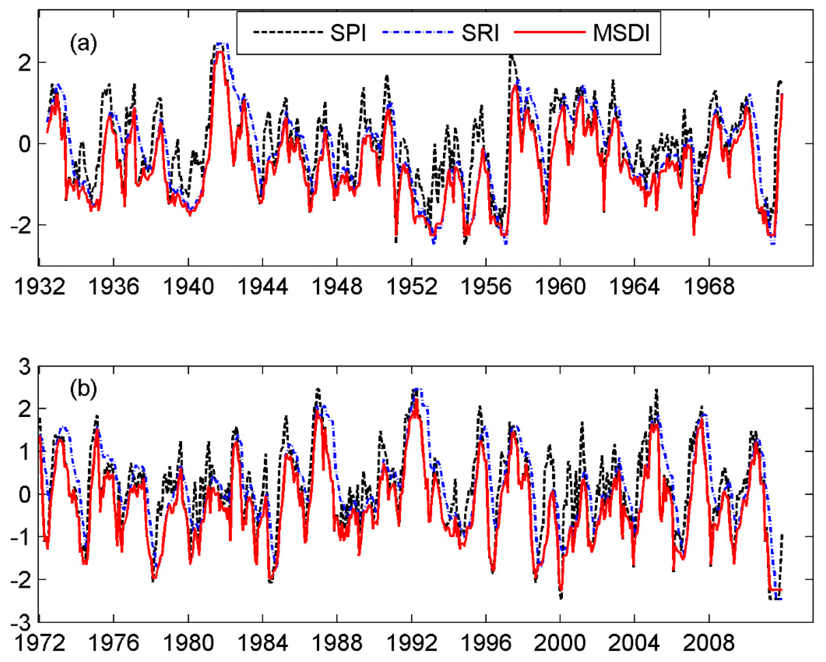
To illustrate the application of the MSDI, monthly precipitation and runoff data for climate division 2 in Texas, USA were used to compute the MSDI based on the SPI and SRI, as shown in Figure 6. It can be seen that when both meteorological and hydrological droughts show deficit, the concurrent drought is more severe than those from SPI and SRI. The usefulness of MSDI partly resides in that it enables to compare the severity of composite drought condition. For July 1936 and 1940 with SPI and SRI values (−0.91, −0.27) and (−0.54, −1.39), it is not straightforward to define the overall drought severity of these two periods (the SPI is more severe for the first period, while the SRI is more severe for the second period). The MSDI for the two periods are −1.04 and −1.50, respectively, indicating that the compound drought for July 1940 are more severe than that for July 1936.
3.4. Quantile Regression
The linear regression has been commonly used to explore the relationship between the response variable and predictors. However, it only estimates the rate of change in the mean of the response variable and thus is generally not suitable for exploring the relationship between extremes. The quantile regression is capable of estimating the functional relationship between the response variable and predictors for all portions of the data and is flexible in modeling data with heterogeneous variance or conditional distribution [154,155].
The quantile regression of a response variable Y as a function of predictor X is introduced as follows [39]. In the traditional linear regression, the conditional mean of Y is related linearly to X as:
where α and β are the intercept and the slope parameters, respectively.
For the quantile regression, quantile τ of the response variable Y conditioned on X is used instead, i.e., Qτ(Y|X). Specifically, for any quantile τ in (0,1), the quantile regression can be expressed as:
where ατ and βτ are the parameters associated with quantile τ. By changing quantile τ, the relationship between Y and X can be explored.
In studying compound extremes, the regression of high (or low) quantile of Y with respect to X is generally of particular interest. In the past decade, the quantile regression has been commonly used to assess the relationship between two extremes or variables, such as soil moisture deficit and temperature extremes (or drought and hot extremes) [38,39,156,157] or rainfall frequency and hot days [158]. For example, extensive studies have shown that the antecedent dry condition (or low soil moisture/precipitation) may induce or intensify the heat wave or high temperature in different regions including Australia [159], Europe [39], and Oklahoma, USA [157], leading to the compound drought and hot extremes.
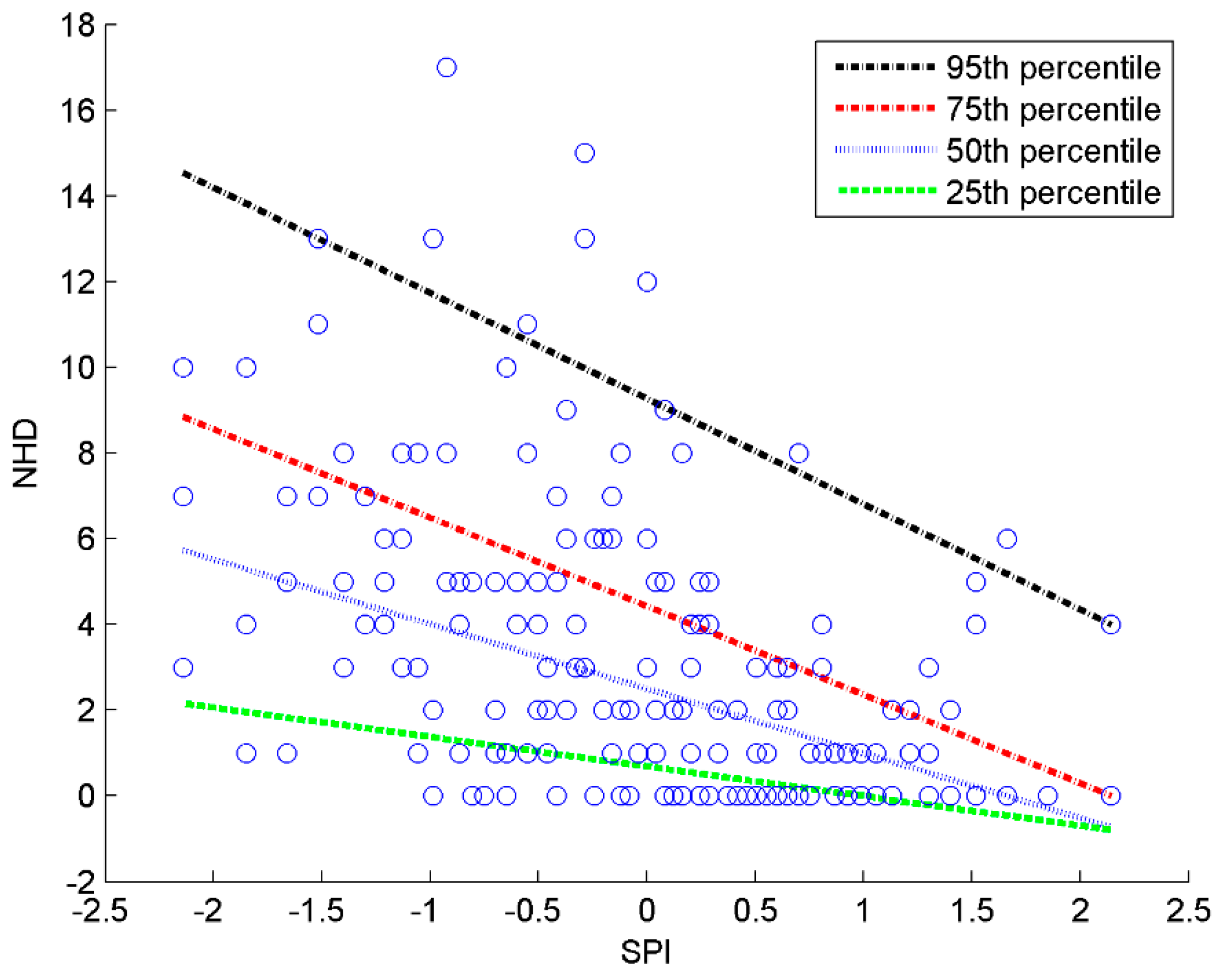
As an example, based on monthly precipitation and daily maximum temperature for one grid (99.625 E, 30.875 N) in northeastern China (data obtained from [160]), the hot extremes in terms of the number of hot days (NHD) during summer months of June, July, and August (JJA) and an antecedent drought indicator SPI for May, June, and July (MJJ) were obtained from these data. The quantile regression of NHD with respect to different SPI values during summer for different quantiles (i.e., 95th, 75th, 50th, and 25th percentile) is shown in Figure 7. It can be seen that there is an overall negative relationship between NHD and SPI indicated by the negative regression slope. The negative dependence increases toward higher quantiles of NHD, which is more sensitive to the antecedent drought condition. These results reveal the impact of drought on hot extremes in that the dry surface condition intensifies hot extremes in this grid, from which the occurrence of compound drought and hot extremes is partly explained.
3.5. Markov Chain Model
The Markov Chain model is commonly used to describe a sequence of possible events in which the present state only depends on the antecedent state. It has been employed to analyze the variability of the individual variable or extreme, such as a drought [161] or a heat wave [162]. A variety of quantities, such as periodicity, persistence, or recurrence time, of the underlying sequence can be defined for characterizing the variables of interest.
A discrete stochastic process Xt (t > 0) with each random variable taking values in the set S = (1, 2, …, m) is a Markov Chain if [161],
where 1 ≤ i, j, k ≤ m. Denote pij the transition probability of the Markov chain. The transition matrix with element pij can be estimated as:
The transition probability is commonly used for characterizing properties of sequence of Xt (e.g., persistence, recurrence time). For example, the persistence of Xt stays in the state j and will reside in the same state j in the following time step can be expressed as pjj. Recently, the Markov Chain model has been employed to study compound extremes (e.g., heavy precipitation- cold in winter and hot- dry days in summer) for central Europe under changing climate [87].
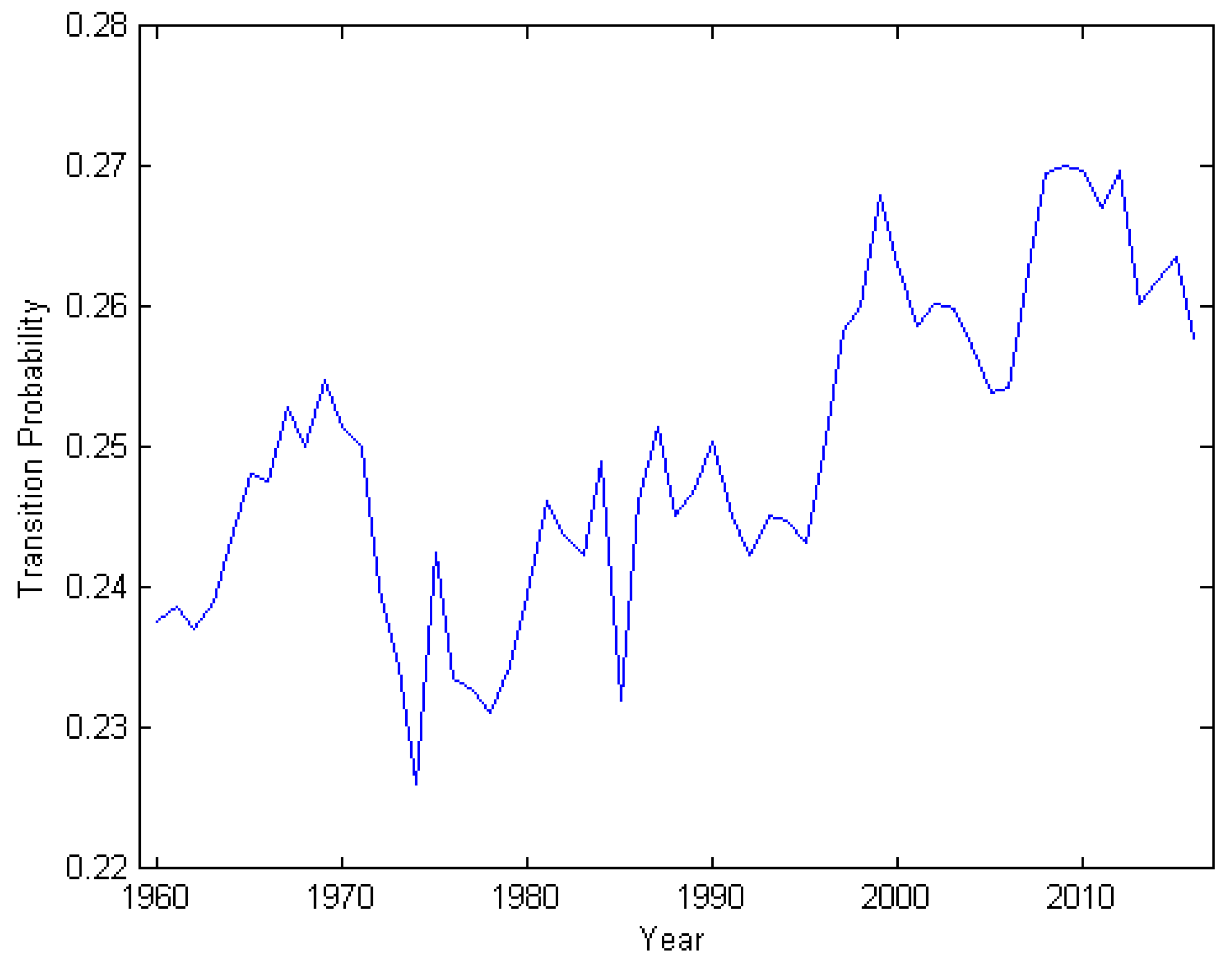
We use the monthly precipitation and temperature data from 1901–2016 near Melbourne, Australia (Longitude: 144.9, Latitude: −37.8) from CRU (TS3.25) to define the compound event of low precipitation and high temperature based on the 50th percentile (i.e., precipitation < 50th percentile and temperature > 50th percentile). The monthly precipitation and temperature series (detrended) are then partitioned in two states (occurrence of compound extreme or not) and a Markov Chain analysis of the occurrence sequence of compound precipitation and temperature sequence was then performed. For illustration purposes, we computed the transition probability for the sequence of every 60 years (i.e., 1901–1960, …, 1957–2016). The temporal variability of the transition probability to compound extreme was shown in Figure 8. The overall increasing of the transition probability indicates that the occurrence of compound extreme is expected to increase under global warming for this grid, which is consistent with previous examples based on the empirical approach.
4. Discussion
4.1. Comparison of Approaches
The approaches introduced above possess different properties in the characterization and modeling of compound extremes. The empirical counting approach and indicator approach have been commonly used to characterize the variability of compound extremes (e.g., occurrence frequency, trend analysis). The empirical approach can be selected when the detection of changes of a compound extreme (e.g., drought and hot extreme) is of primary interest [29]. The indicator approach can be employed to combine different types of extremes for further analysis (e.g., spatial extent [147]). However, they do not describe the interaction between the contributing variables of a compound extreme. The empirical approach usually requires large amounts of data to assess the variation of compound extremes. For 100 data pairs of precipitation and temperature, there would be only 4 co-occurrences of compound dry and hot extremes on average with the 20th and 80th percentile as thresholds of precipitation and temperature if they are assumed to be independent. Observations are usually not abundant enough and the parametric methods, such as the multivariate distribution and quantile regression, can be employed for the statistical extrapolation and inference of compound extremes. The multivariate distribution is capable of modeling the joint behavior of multiple variables or events that lead to the compound extreme. This approach is commonly used for statistical inference and risk assessments of compound extremes based on joint/conditional probability or associated return periods [126,138]. Statistical modeling of multiple extremes through characterizing the dependence among multiple variables or locations is the key in this approach and copula has been among the most commonly used models due to its advantage of flexible dependence modeling. The potential limitation is that most of the commonly used multivariate distributions generally fall short in capturing a complicated dependence in higher dimensions. In an extreme analysis, one is generally interested in the characteristics of a specific quantile (e.g., 80th or 20th percentile) and its relationship with other variables. The quantile regression is advantageous in this case to estimate the relationship between the extreme quantile and the independent variable. However, challenges still remain in the performance of quantile regression in high quantiles (e.g., 99th percentile) due to the limitation of the sample size [163]. The impact of compound extremes depends not only on the number of occurrences but also the sequences of the occurrences [87]. The Markov Chain approach is particularly useful in this case, which enables the characterization of occurrence sequences of different compound extremes.
4.2. High Dimensional Modeling
In this study, most of the compound extremes are introduced in the bivariate case. In reality, there may be multiple variables involved in the occurrence of compound extremes. In this case, one has to model the dependence among a large number of variables (with or without time lags), either at a single location or multiple locations [98]. However, the construction of multivariate distribution in high dimensions remains a challenge (i.e., curse of dimensionality). This calls for suitable tools for dependence modeling in the high dimension to capture a complicated dependence, such as the tail dependence and asymmetric dependence.
The multivariate normal distribution is a traditional model for statistical modeling of multiple random variables even in high dimensions [164]. It is flexible in modeling multiple variables with the dependence structure completely characterized by the variance-covariance matrix, but falls short in modeling complicated dependences (e.g., asymmetric or tail dependence). The multivariate parametric copula is commonly employed for the bivariate case while its extension to higher dimensions (say 4-dimension) is limited in capturing complicated dependence. The vine copula (or the pair-copula construction, PCC), which decomposes the dependence structure into a bivariate dependence that can be modeled with bivariate copulas [165], is among the most recent development in multivariate modeling in a variety of areas [48,166,167,168]. It is expected that the vine copula may provide useful alternatives in modeling compound extremes due to its advantage of flexible dependence modeling even in high dimensions. In addition, the influence diagram, which provides a graphical representation of the conditional dependence and allows the joint distribution of variables to be factorized according to local conditional relationships, is also a potential method for risk estimations of compound extremes in high dimensions [24].
4.3. Compound Extremes Under Climate Change
An important assumption in statistical approaches to model extremes is the stationary assumption of the underlying system [23,169]. It has been highlighted that the fundamental assumption of stationary has been affected by climate change and anthropogenic effects and is not applicable for water resources planning and management [170]. As such, it is advised to check the non-stationary property based on the univariate or multivariate trend analysis using methods such as the (multivariate) Mann–Kendall and Spearman tests [171,172]. The nonstationary property should also be taken into account in the statistical modeling of compound extremes (e.g., frequency analysis). A commonly used method is to incorporate the non-stationary property as covariates [173,174,175,176,177]. For example, the dynamical copula model has been employed for the compound or multivariate extreme analysis with the copula parameter (or parameters of marginal distributions) varying with time [172,173,177].
Assessment of the climate change impact on compound extremes in a hydroclimatic framework is of particular importance for adaptation measures due to their tendency to have a larger impact than an individual extreme [3]. Efforts in assessing the variation of the compound extreme in the future have been growing based on climate projections [28,77,87]. For example, an overall increase of the number of incidences of compound drought and extreme heat is shown for the projection period (2021–2050) over central Europe [28]. In addition, a substantial increase in US East coast flood hazard is expected to occur over the twenty-first century based on the joint projections of the US East coast sea level and storm surge [178]. Research along this line also includes the climate change impact on the dependence structure of multiple variables or extremes, which may affect the risk of compound extremes [179,180,181]. An uncertainty quantification of the impact on the compound extreme is needed to assess the reliability of the change signal, which can be addressed based on the ensemble simulation from the General Circulation Models (GCMs) or Regional Climate Models (RCMs) [28].
5. Conclusions
Analyses of compound extremes have received increasing attention in recent decades due to the exaggerated impacts of multiple extremes that may occur concurrently or consecutively. In this study, we review commonly used statistical methods for characterizing and modeling compound extremes, including the empirical approach, multivariate distribution, the indicator approach, quantile regression and the Markov Chain model. The purposes, data requirements, pros and cons of different approaches are also elaborated upon. A discussion of related topics on compound extremes, such as climate change impacts, is also provided. This study introduced commonly used tools for the characterization and modeling of compound extremes; however, other methods may also be applied, such as a complex network analysis or the covariate approach [182,183]. In addition, we mainly focused on the statistical approaches in modeling different properties of compound extremes. The dynamical model simulations have also been employed for analyzing occurrences of compound extremes [58,184], such as storm surge and sea level/precipitation.
Future efforts are needed to understand the physical processes that lead to compound extremes based on observations and models. Data availability is a potential challenge in investigating compound extremes, since the occurrence of compound extremes is rare, which limits the accurate identification of long-term changes. This may be partly bypassed through pooling observations from multiple sites or employing ensembles from physical models (or simulations from statistical models) [35,56,185]. In addition, modeling the dependence of multiple variables based on historical records is of particular importance in investigating the occurrence or risk of compound extremes. The incorporation of asymmetric dependence and tail dependence in the statistical modeling of compound extremes is still challenging, especially in high dimensions. Moreover, a potential limitation of global climate model for studying extremes is the low resolution that hinders the representation of smaller scale features potentially relevant to climate and weather extremes. Modeling compound extremes with high spatial resolution (e.g., through statistical downscaling or RCMs) is of great importance for resolving local scale phenomena (or interactions) [24,25]. The limitation in the parameterization of certain physical processes (e.g., convective parameterization) also needs to be addressed in the accurate simulation of compound extremes across a wide range of temporal and spatial scales.
Human activities may also influence the occurrence of certain compound extremes. For example, the negative impact of flood occurring immediately after a long term drought, during which a reservoir should be kept as full as possible, may be exacerbated [186,187,188], as shown in the 2011 flooding of Brisbane, Australia that occurred after an exceptional multiyear drought (or “Millennium Drought”) [189]. Thus, continuous efforts are needed in incorporating the interaction of human activity to mitigate the potential impacts of compound extremes. At last, a variety of studies have assessed the impacts of individual extremes (e.g., drought or heat wave) on different sectors, such as agricultural production, for the mitigation and resilience under global warming. The even larger impact of the compound extreme than that of the individual extreme calls for enhanced assessments of the changes and impacts to alleviate the potential threat caused by compound extremes, especially under a changing climate that may induce more extremes.
Author Contributions
Writing-Original Draft Preparation, Z.H.; Writing-Review & Editing, Z.H., V.S., and F.H.
Funding
This research was funded by National Natural Science Foundation of China (Grant number 41601014) and the Fundamental Research Funds for the Central Universities (Grant number 2017XTCX01).
Acknowledgments
Climate division data used in this study were obtained from the Climate Prediction Center (CPC), National Oceanic and Atmospheric Administration (NOAA) (ftp://ftp.cpc.ncep.noaa.gov/wd51yf/us). The monthly precipitation and temperature data from Climatic Research Unit (CRU) can be obtained from (http://www.cru.uea.ac.uk/data). We thank the editors and anonymous reviewers for the valuable comments and suggestions in different rounds of submissions and revisions of this manuscript.
Conflicts of Interest
The authors declare no conflict of interest.
Appendix A. Types of Compound Extremes

Table A1.
Summary of Different Types of Compound Extremes and Statistical Approaches.
| Type of Compound Extremes | Combined Variables/Events/Extremes | Approaches |
|---|---|---|
| Compound drought and hot extreme | Drought and heat wave (hot days or months, high temperature) [37,38,39,65,90,138,156,157,159] | Empirical approach, Quantile regression, Multivariate distribution |
| Compound precipitation and temperature extreme | Heavy precipitation and cold/warm condition [47,87,184,190] | Empirical approach, Markov Chain approach |
| Low precipitation and high temperature [29,179,181,191] | Empirical approach, Multivariate distribution | |
| Dry-warm/dry-cold/wet-warm/wet-cold condition [29,77,80,192] | Empirical approach | |
| Compound flood | Storm surge and high rainfall [35,57,185,193] | Multivariate distribution |
| Storm surge and high discharge/runoff [48,55,56,60,61,136] | Empirical approach, Indicator approach, Multivariate distribution | |
| Storm surge and sea level [73,178] | Empirical approach, Indicator approach | |
| Sea levels and rainfall/river flow [59,97,136,194] | Multivariate distribution | |
| Compound drought | Deficit from precipitation, soil moisture, runoff or other variables [54,153,195] | Indicator approach, Multivariate distribution |
| Combined drought, moisture surplus, precipitation/temperature, and other extremes | Drought indices, precipitation extremes and temperature extremes [146,147,148,196] | Indicator approach |
References
- Reichstein, M.; Bahn, M.; Ciais, P.; Frank, D.; Mahecha, M.D.; Seneviratne, S.I.; Zscheischler, J.; Beer, C.; Buchmann, N.; Frank, D.C. Climate extremes and the carbon cycle. Nature 2013, 500, 287–295. [Google Scholar] [CrossRef] [PubMed]
- Easterling, D.; Groisman, P.Y.; Karl, T.; Evans, J.; Kunkel, K.; Ambenje, P. Observed variability and trends in extreme climate events: A brief review. Bull. Am. Meteorol. Soc. 2000, 81, 417–425. [Google Scholar] [CrossRef]
- IPCC. Managing the Risks of Extreme Events and Disasters to Advance Climate Change Adaptation (Srex) a Special Report of Working Groups I And II of the Intergovernmental Panel on Climate Change; Cambridge University Press: Cambridge, UK; New York, NY, USA, 2012; p. 582. [Google Scholar]
- Horton, R.M.; Mankin, J.S.; Lesk, C.; Coffel, E.; Raymond, C. A review of recent advances in research on extreme heat events. Curr. Clim. Chang. Rep. 2016, 2, 242–259. [Google Scholar] [CrossRef]
- Burt, T.P.; Howden, N.J.K.; Worrall, F. The changing water cycle: Hydroclimatic extremes in the british isles. Wiley Interdiscip. Rev. Water 2016, 3, 854–870. [Google Scholar] [CrossRef]
- Mishra, A.K.; Singh, V.P. Changes in extreme precipitation in texas. J. Geophys. Res. Atmos. 2010, 115, D14106. [Google Scholar] [CrossRef]
- Heim, R.R. An overview of weather and climate extremes—Products and trends. Weather Clim. Extrem 2015, 10, 1–9. [Google Scholar] [CrossRef]
- Trenberth, K.E.; Dai, A.; van der Schrier, G.; Jones, P.D.; Barichivich, J.; Briffa, K.R.; Sheffield, J. Global warming and changes in drought. Nat. Clim. Chang. 2014, 4, 17–22. [Google Scholar] [CrossRef]
- Beniston, M.; Stephenson, D.B.; Christensen, O.B.; Ferro, C.A.T.; Frei, C.; Goyette, S.; Halsnaes, K.; Holt, T.; Jylhä, K.; Koffi, B. Future extreme events in european climate: An exploration of regional climate model projections. Clim. Chang. 2007, 81, 71–95. [Google Scholar] [CrossRef]
- Zisopoulou, K.; Karalis, S.; Koulouri, M.-E.; Pouliasis, G.; Korres, E.; Karousis, A.; Triantafilopoulou, E.; Panagoulia, D. Recasting of the wef nexus as an actor with a new economic platform and management model. Energy Policy 2018, 119, 123–139. [Google Scholar] [CrossRef]
- Dosio, A.; Mentaschi, L.; Fischer, E.M.; Klaus, W. Extreme heat waves under 1.5 °C and 2 °C global warming. Environ. Res. Lett. 2018, 13, 054006. [Google Scholar] [CrossRef]
- Naumann, G.; Alfieri, L.; Wyser, K.; Mentaschi, L.; Betts, R.A.; Carrao, H.; Spinoni, J.; Vogt, J.; Feyen, L. Global changes in drought conditions under different levels of warming. Geophys. Res. Lett. 2018, 45, 3285–3296. [Google Scholar] [CrossRef]
- Dai, A. Drought under global warming: A review. Wiley Interdiscip. Rev. Clim. Chang. 2011, 2, 45–65. [Google Scholar] [CrossRef]
- Alfieri, L.; Bisselink, B.; Dottori, F.; Naumann, G.; Roo, A.; Salamon, P.; Wyser, K.; Feyen, L. Global projections of river flood risk in a warmer world. Earth's Future 2016, 5, 171–182. [Google Scholar] [CrossRef]
- Rummukainen, M. Changes in climate and weather extremes in the 21st century. Wiley Interdiscip. Rev. Clim. Chang. 2012, 3, 115–129. [Google Scholar] [CrossRef]
- Stott, P. How climate change affects extreme weather events. Science 2016, 352, 1517–1518. [Google Scholar] [CrossRef] [PubMed]
- Trenberth, K.E.; Fasullo, J.T.; Shepherd, T.G. Attribution of climate extreme events. Nat. Clim. Chang. 2015, 5, 725–730. [Google Scholar] [CrossRef]
- Rahmstorf, S.; Coumou, D. Increase of extreme events in a warming world. Proc. Natl. Acad. Sci. USA 2011, 108, 17905–17909. [Google Scholar] [CrossRef] [PubMed] [Green Version]
- Alexander, L.V. Global observed long-term changes in temperature and precipitation extremes: A review of progress and limitations in ipcc assessments and beyond. Weather Clim. Extrem 2016, 11, 4–16. [Google Scholar] [CrossRef]
- Panagoulia, D.; Vlahogianni, E.I. Nonlinear dynamics and recurrence analysis of extreme precipitation for observed and general circulation model generated climates. Hydrol. Proccess. 2014, 28, 2281–2292. [Google Scholar] [CrossRef]
- Panagoulia, D.; Vlahogianni, E.I. Recurrence quantification analysis of extremes of maximum and minimum temperature patterns for different climate scenarios in the mesochora catchment in central-western greece. Atmos. Res. 2018, 205, 33–47. [Google Scholar] [CrossRef]
- Katz, R.; Parlange, M.; Naveau, P. Statistics of extremes in hydrology. Adv. Water Resour. 2002, 25, 1287–1304. [Google Scholar] [CrossRef] [Green Version]
- Katz, R.W. Statistics of extremes in climate change. Clim. Chang. 2010, 100, 71–76. [Google Scholar] [CrossRef]
- Leonard, M.; Westra, S.; Phatak, A.; Lambert, M.; van den Hurk, B.; McInnes, K.; Risbey, J.; Schuster, S.; Jakob, D.; Stafford-Smith, M. A compound event framework for understanding extreme impacts. Wiley Interdiscip. Rev. Clim. Chang. 2014, 5, 113–128. [Google Scholar] [CrossRef]
- Seneviratne, S.I.; Nicholls, N.; Easterling, D.; Goodess, C.M.; Kanae, S.; Kossin, J.; Luo, Y.; Marengo, J.; McInnes, K.; Rahimi, M. Changes in climate extremes and their impacts on the natural physical environment. In Managing the Risks of Extreme Events and Disasters to Advance climate Change Adaptation; Field, C.B., Barros, V., Stocker, T.F., Qin, D., Dokken, D., Ebi, K.L., Mastrandrea, M.D., Mach, K.J., Plattner, G.-K., Allen, S.K., et al., Eds.; A Special Report of Working Groups I And II of the Intergovernmental Panel on Climate Change (IPCC); Cambridge University Press: Cambridge, UK, 2012; pp. 109–230. [Google Scholar]
- McPhillips, L.E.; Chang, H.; Chester, M.V.; Depietri, Y.; Friedman, E.; Grimm, N.B.; Kominoski, J.S.; McPhearson, T.; Méndez-Lázaro, P.; Rosi, E.J.; et al. Defining extreme events: A cross-disciplinary review. Earth’s Future 2018, 6, 441–455. [Google Scholar] [CrossRef]
- Orth, R.; Zscheischler, J.; Seneviratne, S.I. Record dry summer in 2015 challenges precipitation projections in central Europe. Sci. Rep. 2016, 6, 28334. [Google Scholar] [CrossRef] [PubMed]
- Sedlmeier, K.; Feldmann, H.; Schädler, G. Compound summer temperature and precipitation extremes over central Europe. Theor. Appl. Climatol. 2018, 131, 1493–1501. [Google Scholar] [CrossRef]
- Hao, Z.; AghaKouchak, A.; Phillips, T.J. Changes in concurrent monthly precipitation and temperature extremes. Environ. Res. Lett. 2013, 8, 034014. [Google Scholar] [CrossRef] [Green Version]
- Lyon, B. Southern africa summer drought and heat waves: Observations and coupled model behavior. J. Clim. 2009, 22, 6033–6046. [Google Scholar] [CrossRef]
- Albright, T.P.; Pidgeon, A.M.; Rittenhouse, C.D.; Clayton, M.K.; Wardlow, B.D.; Flather, C.H.; Culbert, P.D.; Radeloff, V.C. Combined effects of heat waves and droughts on avian communities across the conterminous United States. Ecosphere 2010, 1, 1–12. [Google Scholar] [CrossRef]
- Livneh, B.; Hoerling, M.P. The physics of drought in the U.S. Central great plains. J. Clim. 2016, 29, 6783–6804. [Google Scholar] [CrossRef]
- Mazzarella, A.; Rapetti, F. Scale-invariance laws in the recurrence interval of extreme floods: An application to the upper po river valley (Northern Italy). J. Hydrol. 2004, 288, 264–271. [Google Scholar] [CrossRef]
- Merz, B.; Aerts, J.; Arnbjerg-Nielsen, K.; Baldi, M.; Becker, A.; Bichet, A.; Blöschl, G.; Bouwer, L.M.; Brauer, A.; Cioffi, F.; et al. Floods and climate: Emerging perspectives for flood risk assessment and management. Nat. Hazards Earth Syst. Sci. 2014, 14, 1921–1942. [Google Scholar] [CrossRef] [Green Version]
- Van den Hurk, B.; van Meijgaard, E.; de Valk, P.; van Heeringen, K.-J.; Gooijer, J. Analysis of a compounding surge and precipitation event in the Netherlands. Environ. Res. Lett. 2015, 10, 035001. [Google Scholar] [CrossRef] [Green Version]
- Martius, O.; Pfahl, S.; Chevalier, C. A global quantification of compound precipitation and wind extremes. Geophys. Res. Lett. 2016, 43, 7709–7717. [Google Scholar] [CrossRef] [Green Version]
- Mazdiyasni, O.; AghaKouchak, A. Substantial increase in concurrent droughts and heatwaves in the United States. Proc. Natl. Acad. Sci. USA 2015, 112, 11484–11489. [Google Scholar] [CrossRef] [PubMed]
- Mueller, B.; Seneviratne, S.I. Hot days induced by precipitation deficits at the global scale. Proc. Natl. Acad. Sci. USA 2012, 109, 12398–12403. [Google Scholar] [CrossRef] [PubMed] [Green Version]
- Hirschi, M.; Seneviratne, S.I.; Alexandrov, V.; Boberg, F.; Boroneant, C.; Christensen, O.B.; Formayer, H.; Orlowsky, B.; Stepanek, P. Observational evidence for soil-moisture impact on hot extremes in southeastern Europe. Nat. Geosci. 2011, 4, 17–21. [Google Scholar] [CrossRef]
- Wahl, T.; Plant, N.G.; Long, J.W. Probabilistic assessment of erosion and flooding risk in the northern Gulf of Mexico. J. Geophys. Res. Oceans 2016, 121, 3029–3043. [Google Scholar] [CrossRef] [Green Version]
- Serafin, K.A.; Ruggiero, P. Simulating extreme total water levels using a time-dependent, extreme value approach. J. Geophys. Res. Oceans 2014, 119, 6305–6329. [Google Scholar] [CrossRef] [Green Version]
- Li, F.; van Gelder, P.H.A.J.M.; Ranasinghe, R.; Callaghan, D.P.; Jongejan, R.B. Probabilistic modelling of extreme storms along the Dutch coast. Coast. Eng. 2014, 86, 1–13. [Google Scholar] [CrossRef]
- Corbella, S.; Stretch, D.D. Simulating a multivariate sea storm using archimedean copulas. Coast. Eng. 2013, 76, 68–78. [Google Scholar] [CrossRef]
- Svensson, C.; Jones, D.A. Dependence between extreme sea surge, river flow and precipitation in eastern Britain. Int. J. Climatol. 2002, 22, 1149–1168. [Google Scholar] [CrossRef] [Green Version]
- Reed, A.J.; Mann, M.E.; Emanuel, K.A.; Lin, N.; Horton, B.P.; Kemp, A.C.; Donnelly, J.P. Increased threat of tropical cyclones and coastal flooding to new york city during the anthropogenic era. Proc. Natl. Acad. Sci. USA 2015, 112, 12610–12615. [Google Scholar] [CrossRef] [PubMed]
- Hiroaki, I.; Yukiko, H.; Dai, Y.; Sanne, M.; Ward, P.J.; Winsemius, H.C.; Martin, V.; Shinjiro, K. Compound simulation of fluvial floods and storm surges in a global coupled river-coast flood model: Model development and its application to 2007 Cyclone Sidr in Bangladesh. J. Adv. Model. Earth Syst. 2017, 9, 1847–1862. [Google Scholar]
- Benestad, R.E.; Haugen, J.E. On complex extremes: Flood hazards and combined high spring-time precipitation and temperature in Norway. Clim. Chang. 2007, 85, 381–406. [Google Scholar] [CrossRef]
- Bevacqua, E.; Maraun, D.; Hobæk Haff, I.; Widmann, M.; Vrac, M. Multivariate statistical modelling of compound events via pair-copula constructions: Analysis of floods in Ravenna (Italy). Hydrol. Earth Syst. Sci. 2017, 21, 2701–2723. [Google Scholar] [CrossRef]
- Trepanier, J.C.; Yuan, J.; Jagger, T.H. The combined risk of extreme tropical cyclone winds and storm surges along the U.S. Gulf of Mexico Coast. J. Geophys. Res. Atmos. 2017, 122, 3299–3316. [Google Scholar] [CrossRef]
- Petroliagkis, T.I. Estimations of statistical dependence as joint return period modulator of compound events. Part I: Storm surge and wave height. Nat. Hazards Earth Syst. Sci. Discuss. 2017, 2017, 1–46. [Google Scholar] [CrossRef]
- Fischer, E.; Knutti, R. Robust projections of combined humidity and temperature extremes. Nat. Clim. Chang. 2012, 3, 126–130. [Google Scholar] [CrossRef]
- Schnell, J.L.; Prather, M.J. Co-occurrence of extremes in surface ozone, particulate matter, and temperature over eastern north America. Proc. Natl. Acad. Sci. USA 2017, 114, 2854–2859. [Google Scholar] [CrossRef] [PubMed]
- Wilhite, D.; Glantz, M. Understanding: The drought phenomenon: The role of definitions. Water Int. 1985, 10, 111–120. [Google Scholar] [CrossRef]
- Hao, Z.; Singh, V.P. Drought characterization from a multivariate perspective: A review. J. Hydrol. 2015, 527, 668–678. [Google Scholar] [CrossRef]
- Klerk, W.J.; Winsemius, H.C.; van Verseveld, W.J.; Bakker, A.M.R.; Diermanse, F.L.M. The co-incidence of storm surges and extreme discharges within the rhine–meuse delta. Environ. Res. Lett. 2015, 10, 035005. [Google Scholar] [CrossRef]
- Kew, S.F.; Selten, F.M.; Lenderink, G.; Hazeleger, W. The simultaneous occurrence of surge and discharge extremes for the rhine delta. Nat. Hazards Earth Syst. Sci. 2013, 13, 2017–2029. [Google Scholar] [CrossRef]
- Wahl, T.; Jain, S.; Bender, J.; Meyers, S.D.; Luther, M.E. Increasing risk of compound flooding from storm surge and rainfall for major US cities. Nat. Clim. Chang. 2015, 5, 1093–1097. [Google Scholar] [CrossRef]
- Muis, S.; Verlaan, M.; Winsemius, H.C.; Aerts, J.C.; Ward, P.J. A global reanalysis of storm surges and extreme sea levels. Nat. Commun. 2016, 7, 11969. [Google Scholar] [CrossRef] [PubMed] [Green Version]
- Bengtsson, L. Probability of combined high sea levels and large rains in Malmö, Sweden, southern Resund. Hydrol. Proccess. 2016, 30, 3172–3183. [Google Scholar] [CrossRef]
- Paprotny, D.; Vousdoukas, M.I.; Morales-Nápoles, O.; Jonkman, S.N.; Feyen, L. Compound flood potential in Europe. Hydrol. Earth Syst. Sci. Discuss. 2018, 2018, 1–34. [Google Scholar] [CrossRef] [Green Version]
- Khanal, S.; Ridder, N.; de Vries, H.; Terink, W.; van den Hurk, B. Storm surge and extreme river discharge: A compound event analysis using ensemble impact modelling. Hydrol. Earth Syst. Sci. Discuss. 2018, 2018, 1–25. [Google Scholar] [CrossRef]
- Svensson, C.; Jones, D.A. Dependence between sea surge, river flow and precipitation in south and west Britain. Hydrol. Earth Syst. Sci. 2004, 8, 973–992. [Google Scholar] [CrossRef] [Green Version]
- Diffenbaugh, N.S.; Swain, D.L.; Touma, D. Anthropogenic warming has increased drought risk in California. Proc. Natl. Acad. Sci. USA 2015, 112, 3931–3936. [Google Scholar] [CrossRef] [PubMed] [Green Version]
- Otkin, J.A.; Anderson, M.C.; Hain, C.; Mladenova, I.E.; Basara, J.B.; Svoboda, M. Examining rapid onset drought development using the thermal infrared–based evaporative stress index. J. Hydrometeorol. 2013, 14, 1057–1074. [Google Scholar] [CrossRef]
- Sharma, S.; Mujumdar, P. Increasing frequency and spatial extent of concurrent meteorological droughts and heatwaves in India. Sci. Rep. 2017, 7, 15582. [Google Scholar] [CrossRef] [PubMed] [Green Version]
- Witte, J.C.; Douglass, A.R.; Silva, A.D.; Torres, O.; Levy, R.; Duncan, B.N. Nasa a-train and terra observations of the 2010 Russian Wildfires. Atmos. Chem. Phys. 2011, 11, 19113–19142. [Google Scholar] [CrossRef]
- Rizhsky, L.; Liang, H.; Mittler, R. The combined effect of drought stress and heat shock on gene expression in Tobacco. Plant Physiol. 2002, 130, 1143–1151. [Google Scholar] [CrossRef] [PubMed]
- Jiang, Y.; Huang, B. Drought and heat stress injury to two cool-season turfgrasses in relation to antioxidant metabolism and lipid peroxidation. Crop Sci. 2001, 41, 436–442. [Google Scholar] [CrossRef]
- Rammig, A.; Wiedermann, M.; Donges, J.F.; Babst, F.; Von Bloh, W.; Frank, D.; Thonicke, K.; Mahecha, M.D. Coincidences of climate extremes and anomalous vegetation responses: Comparing tree ring patterns to simulated productivity. Biogeosciences 2015, 12, 373–385. [Google Scholar] [CrossRef]
- Ciais, P.; Reichstein, M.; Viovy, N.; Granier, A.; Ogée, J.; Allard, V.; Aubinet, M.; Buchmann, N.; Bernhofer, C.; Carrara, A. Europe-wide reduction in primary productivity caused by the heat and drought in 2003. Nature 2005, 437, 529–533. [Google Scholar] [CrossRef] [PubMed]
- Yuan, W.; Cai, W.; Chen, Y.; Liu, S.; Dong, W.; Zhang, H.; Yu, G.; Chen, Z.; He, H.; Guo, W. Severe summer heatwave and drought strongly reduced carbon uptake in Southern China. Sci. Rep. 2016, 6, 18813. [Google Scholar] [CrossRef] [PubMed] [Green Version]
- Koster, R.; Schubert, S.; Suarez, M. Analyzing the concurrence of meteorological droughts and warm periods, with implications for the determination of evaporative regime. J. Clim. 2009, 22, 3331–3341. [Google Scholar] [CrossRef]
- Haigh, I.D.; Wadey, M.P.; Wahl, T.; Ozsoy, O.; Nicholls, R.J.; Brown, J.M.; Horsburgh, K.; Gouldby, B. Spatial and temporal analysis of extreme sea level and storm surge events around the coastline of the UK. Sci. Data 2016, 3, 160107. [Google Scholar] [CrossRef] [PubMed]
- Davison, A.C.; Gholamrezaee, M.M. Geostatistics of extremes. Proc. R. Soc. A Math. Phys. Eng. Sci. 2012, 468, 581–608. [Google Scholar] [CrossRef]
- Cooley, D.; Cisewski, J.; Erhardt, R.J.; Jeon, S.; Mannshardt, E.; Omolo, B.O.; Sun, Y. A survey of spatial extremes: Measuring spatial dependence and modeling spatial effects. REVSTAT 2012, 10, 135–165. [Google Scholar]
- Hawkes, P.J.; Gonzalez-Marco, D.; Sánchez-Arcilla, A.; Prinos, P. Best practice for the estimation of extremes: A review. J. Hydraul. Res. 2008, 46, 324–332. [Google Scholar] [CrossRef]
- Beniston, M. Trends in joint quantiles of temperature and precipitation in Europe since 1901 and projected for 2100. Geophys. Res. Lett. 2009, 36, L07707. [Google Scholar] [CrossRef]
- Miao, C.; Sun, Q.; Duan, Q.; Wang, Y. Joint analysis of changes in temperature and precipitation on the Loess Plateau during the period 1961–2011. Clim. Dyn. 2016, 47, 3221–3234. [Google Scholar] [CrossRef] [Green Version]
- Leng, G.; Tang, Q.; Huang, S.; Zhang, X.; Cao, J. Assessments of joint hydrological extreme risks in a warming climate in China. Int. J. Climatol. 2016, 36, 1632–1642. [Google Scholar] [CrossRef]
- Morán-Tejeda, E.; Herrera, S.; López-Moreno, J.I.; Revuelto, J.; Lehmann, A.; Beniston, M. Evolution and frequency (1970–2007) of combined temperature–precipitation modes in the Spanish mountains and sensitivity of snow cover. Reg. Environ. Chang. 2013, 13, 873–885. [Google Scholar] [CrossRef]
- Schär, C.; Ban, N.; Fischer, E.M.; Rajczak, J.; Schmidli, J.; Frei, C.; Giorgi, F.; Karl, T.R.; Kendon, E.J.; Tank, A.M.G.K. Percentile indices for assessing changes in heavy precipitation events. Clim. Chang. 2016, 137, 1–16. [Google Scholar] [CrossRef]
- Zhang, X.; Alexander, L.; Hegerl, G.C.; Jones, P.; Tank, A.K.; Peterson, T.C.; Trewin, B.; Zwiers, F.W. Indices for monitoring changes in extremes based on daily temperature and precipitation data. Wiley Interdiscip. Rev. Clim. Chang. 2011, 2, 851–870. [Google Scholar] [CrossRef]
- Frich, P.L.; Lv, A.; Della-Marta, P.; Gleason, B.; Haylock, M.; Klein, T.A.; Peterson, T.C. Observed coherent changes in climatic extremes during 2nd half of the 20th century. Clim. Res. 2002, 19, 193–212. [Google Scholar] [CrossRef]
- Tank, A.M.G.K.; Wijngaard, J.B.; Können, G.P.; Böhm, R.; Demarée, G.; Gocheva, A.A.; Mileta, M.; Pashiardis, S.; Hejkrlik, L.; Kern-Hansen, C. Daily surface air temperature and precipitation dataset 1901–1999 for European Climate Assessment (ECA). Int. J. Climatol. 2002, 22, 1441–1453. [Google Scholar]
- Alexander, L.; Zhang, X.; Peterson, T.; Caesar, J.; Gleason, B.; Klein Tank, A.; Haylock, M.; Collins, D.; Trewin, B.; Rahimzadeh, F. Global observed changes in daily climate extremes of temperature and precipitation. J. Geophys. Res. 2006, 111, D05109. [Google Scholar] [CrossRef]
- Sunyer, M.A.; Sørup, H.J.D.; Christensen, O.B.; Madsen, H.; Rosbjerg, D.; Mikkelsen, P.S.; Arnbjerg-Nielsen, K. On the importance of observational data properties when assessing regional climate model performance of extreme precipitation. Hydrol. Earth Syst. Sci. 2013, 17, 4323–4337. [Google Scholar] [CrossRef] [Green Version]
- Sedlmeier, K.; Mieruch, S.; Schädler, G.; Kottmeier, C. Compound extremes in a changing climate-a markov chain approach. Nonlinear Process. Geophys. 2016, 23, 375–390. [Google Scholar] [CrossRef]
- Donat, M.G.; Sillmann, J.; Wild, S.; Alexander, L.V.; Lippmann, T.; Zwiers, F.W. Consistency of temperature and precipitation extremes across various global gridded in situ and reanalysis datasets. J. Clim. 2014, 27, 5019–5035. [Google Scholar] [CrossRef]
- Hofstra, N.; New, M.; McSweeney, C. The influence of interpolation and station network density on the distributions and trends of climate variables in gridded daily data. Clim. Dyn. 2010, 35, 841–858. [Google Scholar] [CrossRef]
- Kirono, D.G.C.; Hennessy, K.J.; Grose, M. Increasing risk of months with low rainfall and high temperature in southeast Australia for the past 150 years. Clim. Risk Manag. 2017, 16, 10–21. [Google Scholar] [CrossRef]
- Trepanier, J.C.; Needham, H.F.; Elsner, J.B.; Jagger, T.H. Combining surge and wind risk from hurricanes using a copula model: An example from Galveston, texas. Prof. Geogr. 2015, 67, 52–61. [Google Scholar] [CrossRef]
- Tebaldi, C.; Sansó, B. Joint projections of temperature and precipitation change from multiple climate models: A hierarchical Bayesian approach. J. R. Stat. Soc. Ser. A 2009, 172, 83–106. [Google Scholar] [CrossRef]
- Sexton, D.M.H.; Murphy, J.M.; Collins, M.; Webb, M.J. Multivariate probabilistic projections using imperfect climate models part I: Outline of methodology. Clim. Dyn. 2011, 38, 1–30. [Google Scholar] [CrossRef]
- Watterson, I. Calculation of joint pdfs for climate change with properties matching recent Australian projections. Aust. Meteorol. Oceanogr. J. 2011, 61, 211–219. [Google Scholar] [CrossRef]
- Estrella, N.; Menzel, A. Recent and future climate extremes arising from changes to the bivariate distribution of temperature and precipitation in Bavaria, Germany. Int. J. Climatol. 2013, 33, 1687–1695. [Google Scholar] [CrossRef]
- Rodrigo, F. On the covariability of seasonal temperature and precipitation in Spain, 1956–2005. Int. J. Climatol. 2015, 35, 3362–3370. [Google Scholar] [CrossRef]
- Hawkes, P.J. Joint probability analysis for estimation of extremes. J. Hydraul. Res. 2008, 46, 246–256. [Google Scholar] [CrossRef]
- Hao, Z.; Singh, V.P. Review of dependence modeling in hydrology and water resources. Prog. Phys. Geogr. 2016, 40, 549–578. [Google Scholar] [CrossRef]
- Joe, H. Multivariate Models and Dependence Concepts; Chapman & Hall: London, UK, 1997. [Google Scholar]
- Kao, S.C.; Govindaraju, R.S. Trivariate statistical analysis of extreme rainfall events via the Plackett Family of copulas. Water Resour. Res. 2008, 44, W02415. [Google Scholar] [CrossRef]
- Song, S.; Singh, V. Frequency analysis of droughts using the plackett copula and parameter estimation by genetic algorithm. Stoch. Environ. Res. Risk Assess. 2010, 24, 783–805. [Google Scholar] [CrossRef]
- Chebana, F.; Ouarda, T. Multivariate quantiles in hydrological frequency analysis. Environmetrics 2011, 22, 63–78. [Google Scholar] [CrossRef] [Green Version]
- Mishra, A.K.; Ines, A.V.M.; Das, N.N.; Prakash Khedun, C.; Singh, V.P.; Sivakumar, B.; Hansen, J.W. Anatomy of a local-scale drought: Application of assimilated remote sensing products, crop model, and statistical methods to an agricultural drought study. J. Hydrol. 2015, 526, 15–29. [Google Scholar] [CrossRef]
- Schöelzel, C.; Friederichs, P. Multivariate non-normally distributed random variables in climate research–introduction to the copula approach. Nonlinear Process. Geophys. 2008, 15, 761–772. [Google Scholar] [CrossRef]
- Durante, F.; Salvadori, G. On the construction of multivariate extreme value models via copulas. Environmetrics 2010, 21, 143–161. [Google Scholar] [CrossRef]
- Song, S.; Singh, V.P. Meta-elliptical copulas for drought frequency analysis of periodic hydrologic data. Stoch. Environ. Res. Risk Assess. 2010, 24, 425–444. [Google Scholar] [CrossRef]
- Jonathan, P.; Ewans, K. Statistical modelling of extreme ocean environments for marine design: A review. Ocean Eng. 2013, 62, 91–109. [Google Scholar] [CrossRef]
- Renard, B.; Lang, M. Use of a gaussian copula for multivariate extreme value analysis: Some case studies in hydrology. Adv. Water Resour. 2007, 30, 897–912. [Google Scholar] [CrossRef]
- Rueda, A.; Camus, P.; Tomás, A.; Vitousek, S.; Méndez, F.J. A multivariate extreme wave and storm surge climate emulator based on weather patterns. Ocean Model. 2016, 104, 242–251. [Google Scholar] [CrossRef]
- Bardossy, A. Copula-based geostatistical models for groundwater quality parameters. Water Resour. Res. 2006, 42. [Google Scholar] [CrossRef] [Green Version]
- Bardossy, A.; Li, J. Geostatistical interpolation using copulas. Water Resour. Res. 2008, 44, W07412. [Google Scholar] [CrossRef]
- Kazianka, H.; Pilz, J. Spatial interpolation using copula-based geostatistical models. In geoENV VII—Geostatistics for Environmental Applications; Atkinson, P., Lloyd, C., Eds.; Springer: Dordrecht, The Netherlands, 2010; pp. 307–319. [Google Scholar]
- Nelsen, R.B. An Introduction to Copulas; Springer: New York, NY, USA, 2006. [Google Scholar]
- Trivedi, P.K.; Zimmer, D.M. Copula modeling: An introduction for practitioners. Found. Trends Econom. 2005, 1, 1–111. [Google Scholar] [CrossRef]
- Serinaldi, F.; Bárdossy, A.; Kilsby, C.G. Upper tail dependence in rainfall extremes: Would we know it if we saw it? Stoch. Environ. Res. Risk Assess. 2015, 29, 1211–1233. [Google Scholar] [CrossRef]
- Genest, C.; Kojadinovic, I.; Nešlehová, J.; Yan, J. A goodness-of-fit test for bivariate extreme-value copulas. Bernoulli 2011, 17, 253–275. [Google Scholar] [CrossRef]
- Salvadori, G.; de Michele, C.; Kottegoda, N.; Rosso, R. Extremes in Nature: An. Approach Using Copulas; Springer: New York, NY, USA, 2007. [Google Scholar]
- Cormier, E.; Genest, C.; Nešlehová, J.G. Using b-splines for nonparametric inference on bivariate extreme-value copulas. Extremes 2014, 17, 633–659. [Google Scholar] [CrossRef]
- Genest, C.; Rivest, L.-P. A characterization of gumbel’s family of extreme value distributions. Stat. Probab. Lett. 1989, 8, 207–211. [Google Scholar] [CrossRef]
- Singh, V.P.; Jain, S.K.; Tyagi, A. Risk and Reliability Analysis: A Handbook for Civil and Environmental Engineers; ASCE Press: Reston, VA, USA, 2007. [Google Scholar]
- Singh, V.P. Handbook of Applied Hydrology; McGraw Hill Professional: New York, NY, USA, 2016. [Google Scholar]
- Serinaldi, F. An uncertain journey around the tails of multivariate hydrological distributions. Water Resour. Res. 2013, 49, 6527–6547. [Google Scholar] [CrossRef] [Green Version]
- Mazzarella, A. A fractal approach to sea-surge occurrences in the Northern Adriatic Sea. J. Coast. Res. 1998, 14, 1265–1268. [Google Scholar]
- Malamud, B.D.; Turcotte, D.L. The applicability of power-law frequency statistics to floods. J. Hydrol. 2006, 322, 168–180. [Google Scholar] [CrossRef]
- Mazzarella, A.; Diodato, N. The alluvial events in the last two centuries at Sarno, Southern Italy: Their classification and power-law time-occurrence. Theor. Appl. Climatol. 2002, 72, 75–84. [Google Scholar] [CrossRef]
- Salvadori, G.; Durante, F.; Michele, C. Multivariate return period calculation via survival functions. Water Resour. Res. 2013, 49, 2308–2311. [Google Scholar] [CrossRef] [Green Version]
- Gräler, B.; Petroselli, A.; Grimaldi, S.; De Baets, B.; Verhoest, N. An update on multivariate return periods in hydrology. Proc. Int. Assoc. Hydrol. Sci. 2016, 373, 175–178. [Google Scholar] [CrossRef] [Green Version]
- Serinaldi, F. Dismissing return periods! Stoch. Environ. Res. Risk Assess. 2015, 29, 1179–1189. [Google Scholar] [CrossRef]
- Brunner, M.I.; Seibert, J.; Favre, A.C. Bivariate return periods and their importance for flood peak and volume estimation. Wiley Interdiscip. Rev. Water 2016, 3, 819–833. [Google Scholar] [CrossRef]
- Gräler, B.; van den Berg, M.; Vandenberghe, S.; Petroselli, A.; Grimaldi, S.; De Baets, B.; Verhoest, N. Multivariate return periods in hydrology: A critical and practical review focusing on synthetic design hydrograph estimation. Hydrol. Earth Syst. Sci. 2013, 17, 1281–1296. [Google Scholar] [CrossRef] [Green Version]
- Hao, Z.; Hao, F.; Singh, V.P.; Wei, O.; Cheng, H. An integrated package for drought monitoring, prediction and analysis to aid drought modeling and assessment. Environ. Model. Softw. 2017, 91, 199–209. [Google Scholar] [CrossRef]
- Salvadori, G.; Durante, F.; de Michele, C.; Bernardi, M.; Petrella, L. A multivariate copula-based framework for dealing with hazard scenarios and failure probabilities. Water Resour. Res. 2016, 52, 3701–3721. [Google Scholar] [CrossRef]
- McKee, T.B.; Doesken, N.J.; Kleist, J. The Relationship of Drought Frequency and Duration to Time Scales. In Proceedings of the Eighth Conference on Applied Climatology, Anaheim, CA, USA, 17–22 January 1993; pp. 179–184. [Google Scholar]
- Shukla, S.; Wood, A.W. Use of a standardized runoff index for characterizing hydrologic drought. Geophys. Res. Lett. 2008, 35, L02405. [Google Scholar] [CrossRef]
- Hao, Z.; AghaKouchak, A. Multivariate standardized drought index: A parametric approach for drought analysis. Adv. Water Resour. 2013, 57, 12–18. [Google Scholar] [CrossRef]
- Moftakhari, H.R.; Salvadori, G.; AghaKouchak, A.; Sanders, B.F.; Matthew, R.A. Compounding effects of sea level rise and fluvial flooding. Proc. Natl. Acad. Sci. USA 2017, 114, 9785–9790. [Google Scholar] [CrossRef] [PubMed] [Green Version]
- Koster, R.D.; Wang, H.; Schubert, S.D.; Suarez, M.J.; Mahanama, S. Drought-induced warming in the continental United States under different SST regimes. J. Clim. 2009, 22, 5385–5400. [Google Scholar] [CrossRef]
- Hao, Z.; Hao, F.; Singh, V.P.; Ouyang, W. Quantitative risk assessment of the effects of drought on extreme temperature in Eastern China. J. Geophys. Res. Atmos. 2017, 122, 9050–9059. [Google Scholar] [CrossRef]
- Heffernan, J.E.; Tawn, J.A. A conditional approach for multivariate extreme values (with discussion). J. R. Stat. Soc. B 2004, 66, 497–546. [Google Scholar] [CrossRef] [Green Version]
- Heffernan, J.E.; Resnick, S.I. Limit laws for random vectors with an extreme component. Ann. Appl. Probab. 2007, 17, 537–571. [Google Scholar] [CrossRef]
- Keef, C.; Papastathopoulos, I.; Tawn, J.A. Estimation of the conditional distribution of a multivariate variable given that one of its components is large: Additional constraints for the heffernan and tawn model. J. Multivar. Anal. 2013, 115, 396–404. [Google Scholar] [CrossRef]
- Cheng, L.; Gilleland, E.; Heaton, M.J.; AghaKouchak, A. Empirical bayes estimation for the conditional extreme value model. Stat 2014, 3, 391–406. [Google Scholar] [CrossRef]
- Zhang, L.; Singh, V.P. Bivariate rainfall frequency distributions using archimedean copulas. J. Hydrol. 2007, 332, 93–109. [Google Scholar] [CrossRef]
- Yue, S.; Rasmussen, P. Bivariate frequency analysis: Discussion of some useful concepts in hydrological application. Hydrol. Proccess. 2002, 16, 2881–2898. [Google Scholar] [CrossRef]
- Sillmann, J.; Kharin, V.V.; Zhang, X.; Zwiers, F.W.; Bronaugh, D. Climate extremes indices in the CMIP5 multimodel ensemble: Part 1. Model evaluation in the present climate. J. Geophys. Res. Atmos. 2013, 118, 1716–1733. [Google Scholar] [CrossRef] [Green Version]
- Gallant, A.J.E.; Karoly, D.J. A combined climate extremes index for the Australian Region. J. Clim. 2010, 23, 6153–6165. [Google Scholar] [CrossRef]
- Gallant, A.J.; Karoly, D.J.; Gleason, K.L. Consistent trends in a modified climate extremes index in the United States, Europe, and Australia. J. Clim. 2014, 27, 1379–1394. [Google Scholar] [CrossRef]
- Karl, T.R.; Knight, R.W.; Easterling, D.R.; Quayle, R.G. Indices of climate change for the United States. Bull. Am. Meteorol. Soc. 1996, 77, 279–292. [Google Scholar] [CrossRef]
- Perkins, S.E.; Alexander, L.V. On the measurement of heat waves. J. Clim. 2013, 26, 4500–4517. [Google Scholar] [CrossRef]
- Brooks, H.E.; Lee, J.W.; Craven, J.P. The spatial distribution of severe thunderstorm and tornado environments from global reanalysis data. Atmos. Res. 2003, 67, 73–94. [Google Scholar] [CrossRef]
- Brooks, H.E. Proximity soundings for severe convection for Europe and the United States from reanalysis data. Atmos. Res. 2009, 93, 546–553. [Google Scholar] [CrossRef]
- Coles, S. An Introduction to Statistical Modeling of Extreme Values; Springer: London, UK, 2001. [Google Scholar]
- Kao, S.C.; Govindaraju, R.S. A copula-based joint deficit index for droughts. J. Hydrol. 2010, 380, 121–134. [Google Scholar] [CrossRef]
- Koenker, R.; Bassett, G., Jr. Regression quantiles. Econometrica 1978, 46, 33–50. [Google Scholar] [CrossRef]
- Koenker, R. Quantile Regression; Cambridge University Press: Cambridge, UK, 2005. [Google Scholar]
- Meng, L.; Shen, Y. On the relationship of soil moisture and extreme temperatures in East China. Earth Interact. 2014, 18, 1–20. [Google Scholar] [CrossRef]
- Ford, T.W.; Quiring, S.M. In situ soil moisture coupled with extreme temperatures: A study based on the Oklahoma mesonet. Geophys. Res. Lett. 2014, 41, 4727–4734. [Google Scholar] [CrossRef]
- Quesada, B.; Vautard, R.; Yiou, P.; Hirschi, M.; Seneviratne, S.I. Asymmetric European summer heat predictability from wet and dry southern winters and springs. Nat. Clim. Chang. 2012, 2, 736–741. [Google Scholar] [CrossRef]
- Herold, N.; Kala, J.; Alexander, L. The influence of soil moisture deficits on Australian heatwaves. Environ. Res. Lett 2016, 11, 064003. [Google Scholar] [CrossRef] [Green Version]
- Zhang, X.-J.; Tang, Q.; Pan, M.; Tang, Y. A long-term land surface hydrologic fluxes and states dataset for China. J. Hydrometeorol. 2014, 15, 2067–2084. [Google Scholar] [CrossRef]
- Steinemann, A. Drought indicators and triggers: A stochastic approach to evaluation. J. Am. Water Resour. Assoc. 2003, 39, 1217–1233. [Google Scholar] [CrossRef]
- Shaby, B.A.; Reich, B.J.; Cooley, D.; Kaufman, C.G. A markov-switching model for heat waves. Ann. Appl. Stat. 2016, 10, 74–93. [Google Scholar] [CrossRef]
- Friederichs, P.; Hense, A. Statistical downscaling of extreme precipitation events using censored quantile regression. Mon. Weather Rev. 2007, 135, 2365–2378. [Google Scholar] [CrossRef]
- Wilks, D.S. Statistical Methods in the Atmospheric Sciences; Academic Press: San Diego, CA, USA, 2011; Volume 100. [Google Scholar]
- Aas, K.; Czado, C.; Frigessi, A.; Bakken, H. Pair-copula constructions of multiple dependence. Insur. Math. Econ. 2009, 44, 182–198. [Google Scholar] [CrossRef] [Green Version]
- Liu, Z.; Törnros, T.; Menzel, L. A probabilistic prediction network for hydrological drought identification and environmental flow assessment. Water Resour. Res. 2016, 52, 6243–6262. [Google Scholar] [CrossRef]
- Brechmann, E.C.; Schepsmeier, U. Modeling dependence with C-and D-vine copulas: The R-package cdvine. J. Stat. Softw. 2013, 52, 1–27. [Google Scholar] [CrossRef]
- Liu, Z.; Zhou, P.; Chen, X.; Guan, Y. A multivariate conditional model for streamflow prediction and spatial precipitation refinement. J. Geophys. Res. Atmos. 2015, 120, 10116–10129. [Google Scholar] [CrossRef]
- Milly, P.C.D.; Betancourt, J.; Falkenmark, M.; Hirsch, R.M.; Kundzewicz, Z.W.; Lettenmaier, D.P.; Stouffer, R.J.; Dettinger, M.D.; Krysanova, V. On critiques of “stationarity is dead: Whither water management?”. Water Resour. Res. 2015, 51, 7785–7789. [Google Scholar] [CrossRef]
- Milly, P.; Betancourt, J.; Falkenmark, M.; Hirsch, R.; Kundzewicz, Z.; Lettenmaier, D.; Stouffer, R. Climate change. Stationarity is dead: Whither water management? Science 2008, 319, 573–574. [Google Scholar] [CrossRef] [PubMed]
- Chebana, F.; Ouarda, T.B.; Duong, T.C. Testing for multivariate trends in hydrologic frequency analysis. J. Hydrol. 2013, 486, 519–530. [Google Scholar] [CrossRef]
- Sarhadi, A.; Ausín, M.C.; Wiper, M.P. A new time-varying concept of risk in a changing climate. Sci. Rep. 2016, 6, 35755. [Google Scholar] [CrossRef] [PubMed]
- Bender, J.; Wahl, T.; Jensen, J. Multivariate design in the presence of non-stationarity. J. Hydrol. 2014, 514, 123–130. [Google Scholar] [CrossRef]
- Jonathan, P.; Ewans, K.; Randell, D. Non-stationary conditional extremes of northern North Sea storm characteristics. Environmetrics 2014, 25, 172–188. [Google Scholar] [CrossRef]
- Jonathan, P.; Randell, D.; Wu, Y.; Ewans, K. Return level estimation from non-stationary spatial data exhibiting multidimensional covariate effects. Ocean Eng. 2014, 88, 520–532. [Google Scholar] [CrossRef]
- Jiang, C.; Xiong, L.; Xu, C.Y.; Guo, S. Bivariate frequency analysis of nonstationary low-flow series based on the time-varying copula. Hydrol. Proccess. 2015, 29, 1521–1534. [Google Scholar] [CrossRef]
- Sarhadi, A.; Burn, D.H.; Concepción Ausín, M.; Wiper, M.P. Time-varying nonstationary multivariate risk analysis using a dynamic bayesian copula. Water Resour. Res. 2016, 52, 2327–2349. [Google Scholar] [CrossRef]
- Little, C.M.; Horton, R.M.; Kopp, R.E.; Oppenheimer, M.; Vecchi, G.A.; Villarini, G. Joint projections of us east coast sea level and storm surge. Nat. Clim. Chang. 2015, 5, 1114–1120. [Google Scholar] [CrossRef]
- Zscheischler, J.; Seneviratne, S.I. Dependence of drivers affects risks associated with compound events. Sci. Adv. 2017, 3, e1700263. [Google Scholar] [CrossRef] [PubMed]
- Hao, Z.; Singh, V.P. Integrating entropy and copula theories for hydrologic modeling and analysis. Entropy 2015, 17, 2253–2280. [Google Scholar] [CrossRef]
- Serinaldi, F. Can we tell more than we can know? The limits of bivariate drought analyses in the United States. Stoch. Environ. Res. Risk Assess. 2016, 30, 1691–1704. [Google Scholar] [CrossRef]
- Whan, K.; Zscheischler, J.; Orth, R.; Shongwe, M.; Rahimi, M.; Asare, E.O.; Seneviratne, S.I. Impact of soil moisture on extreme maximum temperatures in Europe. Weather Clim. Extrem 2015, 9, 57–67. [Google Scholar] [CrossRef]
- Sun, A.Y.; Xia, Y.; Caldwell, T.G.; Hao, Z. Patterns of precipitation and soil moisture extremes in Texas, US: A complex network analysis. Adv. Water Resour. 2018, 112, 203–213. [Google Scholar] [CrossRef]
- Tencer, B.; Bettolli, M.L.; Rusticucci, M. Compound temperature and precipitation extreme events in southern South America: Associated atmospheric circulation, and simulations by a multi-rcm ensemble. Clim. Res. 2016, 68, 183–199. [Google Scholar] [CrossRef]
- Zheng, F.; Westra, S.; Sisson, S.A. Quantifying the dependence between extreme rainfall and storm surge in the coastal zone. J. Hydrol. 2013, 505, 172–187. [Google Scholar] [CrossRef]
- Di Baldassarre, G.; Martinez, F.; Kalantari, Z.; Viglione, A. Drought and flood in the anthropocene: Feedback mechanisms in reservoir operation. Earth Syst. Dyn. 2017, 8, 225–233. [Google Scholar] [CrossRef]
- Van Loon, A.F.; Stahl, K.; Di Baldassarre, G.; Clark, J.; Rangecroft, S.; Wanders, N.; Gleeson, T.; Van Dijk, A.I.J.M.; Tallaksen, L.M.; Hannaford, J.; et al. Drought in a human-modified world: Reframing drought definitions, understanding, and analysis approaches. Hydrol. Earth Syst. Sci. 2016, 20, 3631–3650. [Google Scholar] [CrossRef]
- Di Baldassarre, G.; Viglione, A.; Carr, G.; Kuil, L.; Yan, K.; Brandimarte, L.; Blöschl, G. Debates—Perspectives on socio-hydrology: Capturing feedbacks between physical and social processes. Water Resour. Res. 2015, 51, 4770–4781. [Google Scholar] [CrossRef]
- Dijk, A.I.; Beck, H.E.; Crosbie, R.S.; Jeu, R.A.; Liu, Y.Y.; Podger, G.M.; Timbal, B.; Viney, N.R. The millennium drought in southeast Australia (2001–2009): Natural and human causes and implications for water resources, ecosystems, economy, and society. Water Resour. Res. 2013, 49, 1040–1057. [Google Scholar] [CrossRef]
- Tencer, B.; Weaver, A.; Zwiers, F. Joint occurrence of daily temperature and precipitation extreme events over Canada. J. Appl. Meteorol. Climatol. 2014, 53, 2148–2162. [Google Scholar] [CrossRef]
- AghaKouchak, A.; Cheng, L.; Mazdiyasni, O.; Farahmand, A. Global warming and changes in risk of concurrent climate extremes: Insights from the 2014 California drought. Geophys. Res. Lett. 2014, 41, 8847–8852. [Google Scholar] [CrossRef] [Green Version]
- Arsenović, P.; Tošić, I.; Unkašević, M. Trends in combined climate indices in Serbia from 1961 to 2010. Meteorol. Atmos. Phys. 2015, 127, 489–498. [Google Scholar] [CrossRef]
- Zheng, F.; Westra, S.; Leonard, M.; Sisson, S.A. Modeling dependence between extreme rainfall and storm surge to estimate coastal flooding risk. Water Resour. Res. 2014, 50, 2050–2071. [Google Scholar] [CrossRef] [Green Version]
- Lian, J.J.; Xu, K.; Ma, C. Joint impact of rainfall and tidal level on flood risk in a coastal city with a complex river network: A case study of Fuzhou city, China. Hydrol. Earth Syst. Sci. 2013, 17, 679–689. [Google Scholar] [CrossRef]
- Beersma, J.J.; Buishand, T.A. Joint probability of precipitation and discharge deficits in the Netherlands. Water Resour. Res. 2004, 40, W12508. [Google Scholar] [CrossRef]
- Gleason, K.L.; Lawrimore, J.H.; Levinson, D.H.; Karl, T.R.; Karoly, D.J. A revised us climate extremes index. J. Clim. 2008, 21, 2124–2137. [Google Scholar] [CrossRef]
Figure 1.
Different types of compound extremes in the bivariate case for two variables X and Y.

Figure 2.
Number of the compound dry-warm extreme for each year (and 5-year running average) during 1901–2016 for Melbourne, Australia.
Figure 2.
Number of the compound dry-warm extreme for each year (and 5-year running average) during 1901–2016 for Melbourne, Australia.

Figure 3.
Random samples (sample size 1000) from Gaussian, Frank, Clayton, and Gumbel copulas.

Figure 4.
Comparison of individual and compound drought based on the percentile of precipitation and runoff (6-month time scale) for the period 1932–2011 using copula. The circled point represents the data pairs during 2011.
Figure 4.
Comparison of individual and compound drought based on the percentile of precipitation and runoff (6-month time scale) for the period 1932–2011 using copula. The circled point represents the data pairs during 2011.

Figure 5.
Conditional distribution of hydrological drought (represented with SRI) conditioned on the meteorological drought (represented with SPI).
Figure 5.
Conditional distribution of hydrological drought (represented with SRI) conditioned on the meteorological drought (represented with SPI).

Figure 6.
Comparison of drought condition based on SPI, SRI and MSDI in the bivariate case for the period from 1932-2011. (a) 1932–1971; (b) 1972–2011.
Figure 6.
Comparison of drought condition based on SPI, SRI and MSDI in the bivariate case for the period from 1932-2011. (a) 1932–1971; (b) 1972–2011.

Figure 7.
Quantile regression of hot extremes (number of hot days, NHD) with respect to the drought indicator SPI.
Figure 7.
Quantile regression of hot extremes (number of hot days, NHD) with respect to the drought indicator SPI.

Figure 8.
The change of the transition probability to the compound dry and hot extreme during 1960–2016 for Melbourne, Australia.
Figure 8.
The change of the transition probability to the compound dry and hot extreme during 1960–2016 for Melbourne, Australia.

Table 1.
Four copulas and their parameter spaces.
| Copulas | C(u,v) | Parameter |
|---|---|---|
| Gaussian | * | |
| Clayton | ||
| Frank | ||
| Gumbel |
* Φ and Φ2 represent the standard normal distribution in the univariate and bivariate case.
© 2018 by the authors. Licensee MDPI, Basel, Switzerland. This article is an open access article distributed under the terms and conditions of the Creative Commons Attribution (CC BY) license (http://creativecommons.org/licenses/by/4.0/).
Share and Cite
MDPI and ACS Style
Hao, Z.; Singh, V.P.; Hao, F. Compound Extremes in Hydroclimatology: A Review. Water 2018, 10, 718. https://0-doi-org.brum.beds.ac.uk/10.3390/w10060718
AMA Style
Hao Z, Singh VP, Hao F. Compound Extremes in Hydroclimatology: A Review. Water. 2018; 10(6):718. https://0-doi-org.brum.beds.ac.uk/10.3390/w10060718
Chicago/Turabian StyleHao, Zengchao, Vijay P. Singh, and Fanghua Hao. 2018. "Compound Extremes in Hydroclimatology: A Review" Water 10, no. 6: 718. https://0-doi-org.brum.beds.ac.uk/10.3390/w10060718
Note that from the first issue of 2016, this journal uses article numbers instead of page numbers. See further details here.