Article

On the Rainfall Intensity–Duration–Frequency Curves, Partial-Area Effect and the Rational Method: Theory and the Engineering Practice

by
José Nilson B. Campos
,
Ticiana Marinho de Carvalho Studart
*,
Francisco de Assis de Souza Filho
and
Victor Costa Porto
Hydraulic and Environmental Engineering Department (DEHA), Federal University of Ceará, 60020-181 Fortaleza-CE, Brazil
*
Author to whom correspondence should be addressed.
Submission received: 11 September 2020 / Revised: 21 September 2020 / Accepted: 25 September 2020 / Published: 30 September 2020
(This article belongs to the Special Issue Urban Rainwater and Flood Management)

Abstract

:
This research evaluates the partial-area effect and its relationship with the rainfall intensity–duration–frequency (IDF) equations. In the Rational Method, if the critical rainfall duration is shorter than the time of concentration, the partial-area effect occurs. We proved that the partial area could exist for the general ID equation i = a / ( b + t d ) c , only when c > 1 . For these equations, in the application of the Rational Method, the maximum discharge at basin outlet occurs for rainfall duration ( t d ) equal to b/(c−1). Nevertheless, for that case, the Depth Duration Frequency (DDF) has a maximum at that rainfall duration. These situations are present in engineering practice and will be discussed in this paper. Research was done to look for IDF equations with c > 1 in hydrologic engineering practice. It found 640 inconsistent IDF equations ( c > 1 ) in four countries (Brazil, Mexico, India, and USA), which means that a fundamental principle for building consistent IDF equations (i.e., c > 1 ), published in the scientific literature since 1998, did not reach the hydrologic engineering practice fully. We provided some analysis regarding this gap between theory and engineering practice.

Graphical Abstract

1. Introduction

In order to design hydraulic structures, it is necessary to know both peak discharge ( Q p ) and Design Hydrograph ( DH ). The Rational Method plays an important role in the DH estimation and, due to its simplicity, has been extensively applied in engineering practice since the mid-19th century, when it was first introduced and proposed. Nevertheless, researches have recently been questioning basic assumptions of the hydrological theory, including the use of the Rational Method in the existing theoretical framework [1] and the concept of the time of concentration [2], which is the basis for estimating rainfall duration ( t d ) in the Rational Method.
This paper deals with the Rational Method’s assumptions in the context of the partial-area effect, critical rainfall duration, and the relationships of rainfall intensity, duration, and frequency. Usually, the Rational Method is applied for a critical rainfall duration ( t d ) equal to the time of concentration ( t c ) [3,4,5,6,7,8,9,10]. This practice is grounded on the assumption that the partial-area effect does not exist.
The most comprehensive paper published recently that deals with the partial-area effect and critical rainfall duration in the Rational Method framework is due to Wong [11]. He analyzed the equation intensity-duration (ID), i = a / ( t d + b ) , where i is rainfall intensity, t d denotes the rainfall duration, and a and b are equation´s parameters. Wong proved that, for that type of ID equation, there is no partial-area effect, and design discharge is governed by the full-area contribution. In other words, his results are consistent with Rational Method’s engineering practice, where the critical rainfall duration is equal to the time of concentration. Wong’s conclusions, however, are based on the ID equation of the type i = a / ( t d + b ) and, therefore, can only be valid for that type of ID equation. To the best of our knowledge, no article since 2005 has expanded or limited Wong´s conclusions.
The present paper evaluates the partial-area effect for the ID equation i = a / ( t d + b ) c . Koutsoyiannis et al. [12] considered that c ≤ 1 under the constraint that the DD (depth duration rainfall) must be an increasing function over time. A special analysis is dedicated to that case. Research has been done to look for ID equations with c > 1 , since there are numerous c > 1 ID equations in hydrologic engineering practice the world over. However, this suggests that despite the recommendation for building DD consistent equations ( c 1 ), published in the scientific literature since 1998, has not fully become an integral part of hydrologic engineering practice. We provide some analysis to explain why the gap between theory and practice persists.

2. Methods

2.1. The Rational Method

Many authors [13,14,15,16] credit the Rational Method to the work of Mulvany [17], which is regarded as the first rainfall-runoff model. In his paper, Koutsoyiannis et al. [12] explains how to estimate the peak discharge ( Q p ), at the outlet of a basin, from observed rainfall intensity ( i ), given a catchment basin area ( A b ), and given an empirical factor ( C ) that depends on basin soil. In fact, in his paper, Mulvany did not, explicitly, write the equation, but his words can be translated in Equation (1).
Q p = C   × i   × A
where Q p is the maximum discharge at basin outlet, i is the rainfall intensity, and A is the basin area.
Mulvany [17] understood that it was necessary to put limits on the application of the method and stated that this result, although arrived at in an empirical manner, is found to be tolerably near the truth in the catchment of an average character, neither mountainy nor very flat, and within certain limits as to the extent.
Many other researchers throughout the years have also devoted efforts to building a conceptual framework that establishes the boundaries of applying the Rational Method to diverse situations. Ponce [4], for example, suggests that the Rational Method is based on the principle of concentration and diffusion. In the case of concentration without diffusion, uniform precipitation over the basin with duration equal to the time of concentration ( t c ) (design storm) will make the design hydrograph have an isosceles triangle or trapezius shape, depending on the rainfall duration. It must be observed that Ponce’s conceptualization of a hydrograph comes from an overland rectangular plane, and the discharge flows to the outlet at a given constant velocity.
These two examples highlight the importance of understanding the type of ID equation used for cases where the partial-area effect is dominant. The following sections of this paper will be devoted to this task.

2.2. Rainfall Intensity–Duration–Frequency Relationship

The type of Intensity Duration Frequency (IDF) equation is a key point in estimating the DH for an urban drainage structure in small basins, given the limits of applicability of Rational Method. There are many types of IDF equations. A common characteristic of all IDF equations is that the rainfall intensity varies inversely with the rainfall duration. The most general equations found in the literature is synthesized in the form of Equation (2) [7,18]:
i =   K   ×   ( T r ) n ( t d + b ) c
where K ,   b ,   c , and n are equation parameters, T r is the rainfall return period, t d is the rainfall duration. For a given return period, assuming a = K ( T r ) n , we have the ID equation for that T r (Equation (3)):
i =   a ( t d + b ) c

2.3. The Partial-Area Effect

A watershed is governed either by a full-area contribution or by a partial-area contribution. A partial-area contribution [19] is an effect that emerges when the maximum discharge at the basin outlet occurs before the whole watershed is contributing to the discharge outlet. Otherwise, the basin is governed by the full area contribution. The analysis of the partial-area effect and critical rainfall duration is studied based on two parameters: (1) an assumption that basin is either homogeneous or heterogeneous; and (2) an assumption that losses are either constant or proportional to the precipitation.
For heterogeneous basins, the scientific literature [20,21,22,23] unambiguously demonstrates that the critical rainfall duration ( t d ) can and often is different from the time of concentration ( t c ). Thus, for heterogeneous basins, we can be confident in claiming that critical rainfall duration is different from the time of concentration.
In this paper, we discuss the partial-area effect for a plane under the theoretical framework of the Rational Method. The rainfall has duration t d and is under an ID Equation (3). The rectangular plane has area A b and time of concentration t c . Two cases are discussed: (1) t d < t c and (2)   t d = t c .
In case 1, t d < t c , the area of contribution at time t ( A c ( t ) ) and peak discharge ( Q p ( t ) ) increase up to the end of rainfall ( t = t d < t c ). At this instant, A c ( t ) is a fraction of the basin area ( A c ( t d ) < A b ) and the discharge at outlet reaches its maximum Q p ( 1 ) . From t = t d up to t = t c , the values of A c ( t ) and Q p ( 1 ) remains constant. From t = t c to t = t c + t d , A c ( t ) and Q p ( 1 ) decreases up to zero.
In case 2, t d = t c , A c ( t ) and Q p ( t ) increase up to A b and Q p ( 2 ) . At the time t = t c = t d (end of rainfall), all the basin is contributing for the discharge at the outlet. From this time up to t = 2 t c , the discharge decreases to zero.
The key point is to verify if the maximum discharge at the outlet in case 1 is greater than in case 2, for that basin and ID Equation. If Q p ( 1 )   >   Q p ( 2 ) , we say that the partial-area effect exists; otherwise, it does not. Examples with real data are presented to illustrate the case.
To show an example of a partial-area effect in the application of the Rational Method, let us consider the application of the South Bend (South Bend, IN, USA) ID equation, that is valid for t d < 1   h [24] or an urban basin with area A b = 1   km 2 , t c = 1   h and T r = 10 years.
i =   1.7204   ( 10 ) 0.1753 ( t d + 0.485 ) 1.6806
where i is in inches/h and t d in hours.
Let us now compute Q p at basin outlet for rainfall durations t d = 0.71   h and t d = 1   h .
For t d = 0.71   h , the rainfall intensity is 1.91 inches/h, that is equivalent to 0.01348 mm/s. At this time, A c is (0.71/1) × A b (equal to 0.71 km2). Applying the Rational Method, with C = 0.8 we have Q p ( 0.71 ) = 0.8 × 0.01348 × 0.71 × (106/103) = 7.65 m3/s.
For t d = 1   h , the rainfall intensity is 1.32 inches/h, that is equivalent to 0.00935 mm/s. At this time, A c is the basin area (1.0 km2). Applying the Rational Method, with C = 0.8 we have Q p ( 1 ) = 0.8 × 0.00935 × 1.0 × (106/103) = 7.48 m3/s.
The hydrographs used in this example are shown in Figure 1A. It should be noted that the maximum discharge at the outlet occurs with the rainfall duration which the contribution area ( A c ) is 71% of the basin area, and the partial-area effect exists for this ID equation. In Figure 1B, the Depth Duration (DD) graph resulting from the integration of the South Bend ID equation is illustrated, and the DD curve exhibits a maximum at time t d = 0.71   h . Thus, this equation is not consistent for t d > 0.71   h and it is not valid in the interval 0.71 h–1.0 h as it was supposed to be.

2.4. Critical Rainfall Duration for a Given ID Equation in Rational Method Conceptual Framework

The idea is to find, for a given ID equation, if the time t   in which the discharge at outlet reaches the maximum value ( Q p ( t ) ) is a finite value. The time for this maximum will be denoted by t * . If t * exists, then for that equation, the partial-area effect will be present for any area with t c < t * .
Then, we are looking for the maximum of the function Q p ( t ) = C ( a / ( t d + b ) c )   A c ( t ) , if it exists.
This function can be conceptualized at the outlet of a rectangular sufficiently long overland plane (Figure 2). In that plane, the A c ( t ) increases linearly along the time t . The rectangular plane used has length L , width W , and area A b . During the duration t d , the rainfall over the basin has a constant intensity i and is obtained from the ID equation. Let L c ( t ) denote the length of the contributing area at time t . The flow velocity in the outlet direction, which is represented by v , is assumed to be constant and equal to L / t c , so, in Equation (5) L c ( t ) = v   ×   t = ( L t c )   ×   t .
The contributing area to the discharge at the outlet at time t is given as Equations (5) and (6).
A c ( t ) = L c ( t )   ×   W =   L   ×   t t c   ×   W =   A b   ×   t t c ,    f o r    t < t c
where A c ( t ) is the contribution area at time t , L c ( t ) is the length of A c ( t ) , W is the plane wide, and L is the length of the plane.
When the rainfall duration t d   >   t c , all the basin is contributing to the discharge outlet (Equation (6)):
A c ( t ) =   A b ,    f o r    t     t c
Equation (7) estimates the discharge at time t at the basin outlet,
Q p ( t ) = C ×   i ×   A c ( t )
where Q p ( t ) is the discharge at the mouth of the basin at time t , i is the mean rainfall intensity during the rainfall duration, which was calculated from the ID equation, and A c ( t ) is the contributing area at time t .
We developed an analytical equation for estimating the time t * . If t * is less than t c , then the partial-area effect exists. To calculate t * , the derivative d Q ( t ) / d t is set to zero, and this equation is solved for t .
Substituting the data of Equation (4) into Equation (7) results in Equation (8):
Q ( t ) =   C   ×   a ( t + b ) c   v   × t   × W
where symbols were as previously defined. Equation (8) can be rewritten in the form of Equation (9):
Q ( t ) =   J   ×   t ( t + b ) c
where J = C   ×   a   ×   v   × W . Taking the derivative of Q ( t ) with respect to t and making it equal to zero to find a maximum, we have
d Q ( t ) d t =   J ( t + b ) c     J   ×   t   ×   c ( t + b ) c ( t + b ) =   0
solving Equation (10) for t , and denoting the time for the maximum by t * :
t * =   b ( c 1 )
It is clear, from this equation, that the critical time ( t * ) only occurs, in the positive real domain, if c > 1 . For c 1 there is no maximum in the positive domain and Equation (11) shows that the time of maximum discharge is infinite ( t * = ). The conclusion is that for the type of ID equation analyzed, the partial-area effect exists only if c > 1 . On the other hand, the existence of a partial-area effect when c > 1 has the property that the DDF is inconsistent.
Two situations emerge: (1) t * is inside the field of the validity of the ID equation, as shown in Figure 1; and (2) the t * is beyond the limit of validity of the ID equation. The second situation is shown in the example below for the Fort Wayne (Fort Wayne, IN, USA) ID equation, which is also valid for t d   <   1   h [24] under the same basin conditions as the previous example ( A b = 1   km 2 , t c = 1   h   and T r = 10   years):
i =   2.003   ( 10 ) 0.1655 ( t d + 0.516 ) 1.4643
The hydrographs of the Rational Method applied to three different durations (0.5, 0.7, and 1 h) are illustrated in Figure 3A. Although c > 1 , as the decreasing and inconsistent part of the DD curve ( t d > t * = 1.1   h ) occurs after the duration limit of the ID equation (Figure 3B), no partial-area effect occurs in the hydrographs independent of which t d and t c are chosen.

3. Results and Discussions

3.1. On the Consistency of IDF Equation and the Partial-Area Effect

For the general IDF equation be consistent, the depth–duration–frequency DDF must be an increasing function, as represented by Equation (13):
DDF ( t 1 ) =   IDF ( t 1 ) × t 1 < IDF ( t 2 ) × t 2 = DDF ( t 2 )
for any t 1 < t 2 in the field of the validity of the IDF equation.
For a rainfall with duration td the DDF function is given by Equation (14):
DDF ( t ) = IDF ( t ) × t   =   a ( t + b ) c t
Making the DDF ( t ) derivative equal to zero, to find if it has a maximum, we found:
t m   =   b ( c 1 )
where t m is the time where the DDF has a maximum, and b and c are parameters of the IDF equation.
From Equation (15), we conclude that if c > 1 , the DDF function has a maximum in the positive side of the t axis. This is incompatible with the requirement that the DDF should be crescent in the positive t axis. So, for c > 1 , the IDF is not valid for t   ×   b / ( c 1 ) .
With this result in place, we can now ask: are these conceptual limitations inserted in hydrologic engineering practice? Furthermore, if not, how are engineering results impacted? In the next sections, we will answer these questions to show that the partial-area effect can be present in engineering practice, but only for DDF inconsistent relationship.

3.2. The Inexistence of Partial-Area Effect for Any IDF Relationship

To answer the first question proposed in the previous section, we conducted research in an extensive IDF Brazilian database, along with bibliographical research in other countries of the world.
The conceptualization of the partial-area effect for any type of IDF, considering the Rational Method, can be represented by the Equation (16):
C   ×   IDF ( t 1 )   ×   A c ( t 1 ) > C   ×   IDF ( t 2 )   ×   A c ( t 2 )
where IDF ( t 1 ) and IDF ( t 2 ) are the rainfall intensity at the time t 1 and t 2 , respectively, with t 1 < t 2 , and A ( t 1 ) and A ( t 2 ) are the areas contributing to the outlet at the time t 1 and t 2 , respectively.
In the Rational Method conceptual framework the water velocity over the plane is constant (let us assume that it is equal to v p ) and the contribution area at time t is A c ( t ) = v p t . So, Equation (16) can be rewritten as Equation (17).
C × IDF ( t 1 )   × v p   ×   t 1   > C × IDF ( t 2 ) × v p × t 2
Simplifying,
IDF ( t 1 ) × t 1 = DDF ( t 1 ) > IDF ( t 2 ) × t 2 = DDF ( t 2 )
As t 1 <   t 2 , Equation (18) means that the existence of partial effect in any representation of IDF relationship implies in a DDF(t) is decreasing, which is impossible. The conclusion is that in any mathematical representation of IDF, equations or curves, the partial-area effect does not exist.

3.3. IDF Equations with c > 1 in Different Regions of the World

The general IDF equations with c > 1 are not necessarily inconsistent. As empirical equations, they should have a limit of validity. For t < t * the DDF is monotone crescent, and, within that reach, the IDF equations are valid for c > 1 . To evaluate the use of c > 1   in engineering practice, we gathered several IDF equations from the literature. We collected the following data: 544 equations from Brazil, 63 equations from Mexico, 19 stations from India, and 4 peculiar equations from Indiana (USA).
To evaluate the impact of these equations in engineering practice, t * was computed and grouped in four classes: 0–2 h; 2–5 h; 5–24 h, and greater than 24 h. The first two classes are related to errors in Rational Method application; the third class is related to inconsistencies in applications of alternating block hydrograph; the fourth class, besides being inconsistent in DDF, has little application in engineering practice.

3.3.1. The IDF Equations with c > 1 in Brazil

In Brazil, the research covers 544 IDF equations available in the hydrologic software PLUVIO 2.1 database [25]. Seventy-eight of these equations have a c value greater than one. The value of t * was estimated for 80 equations (Table 1 and Table S1). The minimum t * in Brazil is 2.6 h (in the station Conceição da Mata de Dentro in Minas Gerais).

3.3.2. IDF Equations in Mexico

Manzano-Agugliaro et al. (Table S2) [26] assess four methods of obtaining IDF equations for the Mexican case [27,28,29]. In that paper, the Cheng-lung Chen Equation [27] has the same configuration of the general IDF. The problem of limits of consistency ( c > 1 ) is not referred to in that paper. Twenty-seven of the 63 equations present c > 1 and 27 of those are consistent only for t < t * . The authors concluded that Cheng-lung Chen Equation [27] gives good results for rainfall durations between 2 h and 24 h; however, a great number of the equations presented are not valid for that interval as shown in Table 2. Eight of them are not valid if t < 2 h, while 19 resulted in t * < 5 h.

3.3.3. IDF Equations in India

In India, the research covered 19 equations obtained from an Engineering textbook. From these equations, seven (36.6%) have c > 1 . The minimum t * is 3.9 h (Table 3 and Table S3) [30].

3.3.4. IDF Equations in Indiana (USA)

In Indiana, the research covers four regional IDF equations. These equations present a different formulation from all equations previously analyzed. The IDF has two parts: the first is valid for rainfall duration of less than one hour; the second, for rainfall duration greater than one hour and less than 36 h [24]. For the rainfall duration of less than one hour, all equations have c > 1 (Table 4), and c < 1 for t d > 1 h. Two of these equations have t * greater than one hour, and two have t * less than one hour. In other words, the equations for South Bend and Evansville are not valid in the interval 0–1 h, as they are supposed to be.

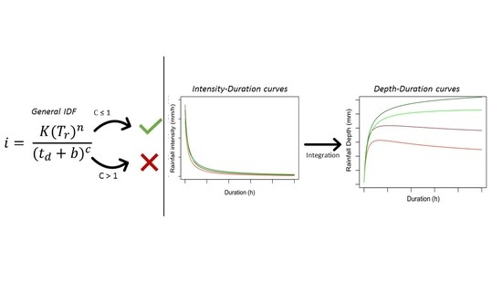
3.4. The IDF and DDF Curves

One conclusion from the prior analysis is that the classical method of developing IDF equations, with the empirical fitting of rainfall duration and intensity, can yield an IDF equation that is DDF inconsistent. Another conclusion is that, just looking to the IDF curves (monotone, decreasing, asymptotic to zero), it is not possible to identify if the DDF is consistent (monotone increasing).
There is a common practice in engineering where the IDF curves of drainage projects are built without the respective IDF equations [31] but built by graphic adjustment alone. The problem with this method, as demonstrated in the previous section, is that an IDF equation may appear consistent even when the DDF equation is inconsistent. It is, therefore, reasonable to be skeptical about the consistency of IDF curves, since they may well contain inconsistent DDFs.
As there is no equation nor c parameter provided, the only way to know if the resulting DDF is consistent is by the graphical integration of the IDF curve, which is not a typical engineering practice.
For the places that present the intense rainfall relationship by DDF curves, there is no problem. The inconsistency, if exists, will be detected at first look, and then corrected.

4. Conclusions

The proof for the inexistence of a partial-area effect in an overland plane with an application of the Rational Method was restricted to a case of the IDF equation [32]. This paper expands that result to show that, for any representation of IDF equations, or even for curves without equations, the partial-area effect only exists for cases with a decreasing reach of the DD function. Nevertheless, conceptually, the DD function should be increasing over the time. In ID equations with c > 1 , the DD has a maximum at t d = t * = b ( c 1 ) , so they do not attend the restriction of increasing DD. In that case, the ID equation is only valid for t d < t * .
Research on 640 IDF equations was done for four countries: Brazil (554 equations), Mexico (63 equations), India (19 equations), and USA (Indiana, 4 equations). For Brazil, from 554 equations, 80 have c > 1 , ten of them are valid only for rainfall duration less than five hours; 61 have validity less than 24 h. For Mexico, from 63 IDF equations, 27 have c > 1 . Eight of them have t * less than two hours, and 26 have t * less than 24 h. For India, from 19 equations, three have t * less than five hours, and six have t * less than 24 h. For Indiana USA, the IDF equations have two ranges for the application. The first range was designed for rainfall durations of less than one hour. In the first range, t d less than one hour. All the equations have c > 1 . Two of them have t * > 1 h, so they are correct; two have t * < 1 h, so they are not valid in the range proposed in the publication.
The inconsistency on the IDF equation with c > 1 has been established in scientific literature since 1998 [12]. Nevertheless, a significant number of IDF equations with c > 1 are available for engineering applications, without comments on their limits of validity. Why this gap between theory and practice? The main bridge between theory and practice is engineering textbooks. We researched several classical hydrological textbooks in the English and Portuguese language (without citation here), and none of them emphasize the limits of validity of the general IDF equation. The classical method for building IDF equations is still in practice, which builds DDF-inconsistent equations.
There is a final point concerning IDF curves. If the empirical fitting of observed rainfall intensities and durations yields equations that look good but are DDF-inconsistent, then it plausible to assume the same occurs in empirical IDF curves. Only by the integration of IDF curves will guarantee that these curves are DDF-consistent. This question remains to be answered in future studies.

Supplementary Materials

The following are available online at https://0-www-mdpi-com.brum.beds.ac.uk/2073-4441/12/10/2730/s1, Table S1: Rainfall intensity-duration-frequency (IDF) Brasil with c > 1; Table S2: Rainfall intensity-duration-frequency (IDF) Mexico with c > 1, and Table S3: Rainfall intensity-duration-frequency (IDF) India with c > 1.

Author Contributions

Conceptualization, methodology, formal analysis, and writing—original draft preparation, J.N.B.C., T.M.d.C.S., and F.d.A.d.S.F.; investigation, J.N.B.C, T.M.d.C.S., F.d.A.d.S.F., and V.C.P.; writing—review and editing, supervision: J.N.B.C., T.M.d.C.S., and F.d.A.d.S.F. All authors have read and agreed to the published version of the manuscript.

Funding

The work of the first author was supported by grant from the Conselho Nacional de Desenvolvimento Científico e Tecnológico—Brasil (CNPq) (n. 303658/2013-4). For the second and third authors it was funded by Conselho Nacional de Desenvolvimento Científico e Tecnológico—Brasil (CNPq)—Research Project SHAE-SF (NEXUS): Segurança Hídrica, Alimentar e Energética na Bacia Estendida do Rio São Francisco (n. 441457/2017-7), by Coordenação de Aperfeiçoamento de Pessoal de Nível Superior—Brasil (CAPES)—Research Project: Impactos das Mudanças Climáticas em Extremos Hidrológicos (Secas e Cheias) (n. 23038.003964/2016-53) and by grants from the Conselho Nacional de Desenvolvimento Científico e Tecnológico—Brasil (CNPq) and Fundação Cearense de Apoio ao Desenvolvimento Científico e Tecnológico (FUNCAP).

Conflicts of Interest

The authors declare no conflict of interest.

References

  1. Grimaldi, S.; Petroselli, A. Avons-nous encore besoin de la formule rationnelle? Une méthode empirique alternative pour l’estimation du débit de pointe dans les petits bassins et les bassins non jaugés. Hydrol. Sci. J. 2014, 60, 67–77. [Google Scholar] [CrossRef]
  2. Grimaldi, S.; Petroselli, A.; Tauro, F.; Porfiri, M. Temps de concentration: Un paradoxe dans l’hydrologie moderne. Hydrol. Sci. J. 2012, 57, 217–228. [Google Scholar] [CrossRef] [Green Version]
  3. Gupta, R.S. Hydrology and Hydraulic Systems; Prentice Hall: Englewood Cliffs, NJ, USA, 1989. [Google Scholar]
  4. Ponce, V.M. Engineering Hydrology: Principles and Practices; Prentice Hall: Englewood Cliffs, NJ, USA, 1989. [Google Scholar]
  5. McCuen, R.H. Hydrologic Analysis and Design, 2nd ed.; Prentice Hall: Englewood Cliffs, NJ, USA, 1998. [Google Scholar]
  6. Nzewi, E.U. The McGraw-Hill Civil Engineering PE Exam Depth Guide: Water Resources; McGraw-Hill: New York, NY, USA, 2001. [Google Scholar]
  7. Campos, J.N.B. Liçoes em Modelo e Simulação Hidrológica; Expressão Gráfica: Fortaleza, Brazil, 2009. [Google Scholar]
  8. Kang, M.S.; Koo, J.H.; Chun, J.A.; Her, Y.G.; Park, S.W.; Yoo, K. Design of drainage culverts considering critical storm duration. Biosyst. Eng. 2009, 104, 425–434. [Google Scholar] [CrossRef]
  9. Brooks, K.N.; Ffolliott, P.F.; Magner, J.A. Hydrology and the Management of Watersheds; Wiley-Blackwell: Oxford, UK, 2012. [Google Scholar]
  10. Maidment, D.R. Handbook of Hydrology; McGraw-Hill Book Company: New York, NY, USA, 1993. [Google Scholar]
  11. Wong, T.S.W. Influence of Loss Model on Design Discharge of Homogeneous Plane. J. Irrig. Drain Eng. 2005, 131, 210–217. [Google Scholar] [CrossRef]
  12. Koutsoyiannis, D.; Kozonis, D.; Manetas, A. A mathematical framework for studying rainfall intensity-duration-frequency relationships. J. Hydrol. 1998, 206, 118–135. [Google Scholar] [CrossRef]
  13. Dooge, J.C. The rational method for estimating flood peaks. Engineering 1957, 184, 311–313. [Google Scholar]
  14. Singh, V.P.; Woolhiser, D.A. Mathematical Modeling of Watershed Hydrology. J. Hydrol. Eng. 2002, 7, 270–292. [Google Scholar] [CrossRef] [Green Version]
  15. Beven, K.J. Rainfall-Runoff Modelling: The Primer; Wiley-Blackwell: Oxford, UK, 2012. [Google Scholar]
  16. Biswas, A.K. History of Hydrology; North-Holland Publishing Co.: Amsterdam, The Netherlands, 1970. [Google Scholar]
  17. Mulvany, T. On the use of self-registering rain and flood gauges in making observations of the relations of rain fall and of flood discharges in a given catchment. Proc. Inst. Civ. Eng. Irel. 1851, 4, 18–33. [Google Scholar]
  18. Chow, V.; Maidment, D.R.; Mays, L.W. Applied Hydrology; McGraw-Hill: New York, NY, USA, 1988. [Google Scholar]
  19. Betson, R.P. What is watershed runoff? J. Geophys. Res. 1964, 69, 1541–1552. [Google Scholar] [CrossRef]
  20. Hinks, R.W.; Mays, L.W. Hydrology for Water Excess Management. In Water Resources Handbook; Mays, L., Ed.; McGraw-Hill: New York, NY, USA, 1996; pp. 23–24. [Google Scholar]
  21. Schmid, B.H. Critical rainfall duration for overland flow from an infiltrating plane surface. J. Hydrol. 1997, 193, 45–60. [Google Scholar] [CrossRef]
  22. Debo, T.N.; Reese, A. Municipal Stormwater Management; CRC Press: Boca Raton, FL, USA, 2002. [Google Scholar] [CrossRef]
  23. Rigon, R.; Odorico, P.; Bertoldi, G. The geomorphic structure of the runoff peak. Hydrol. Earth Syst. Sci. 2011, 15, 1853–1863. [Google Scholar] [CrossRef] [Green Version]
  24. Burke, C.C.; Burke, T.T. Stormwater Drainage Manual 2015; Indiana Local Technical Assistance Program (LTAP) Publications: West Lafayette, IN, USA, 2015. [Google Scholar]
  25. Pruski, F.F.; Teixeira, A.F.; Silva, D.D.; Cecílio, R.A.; Silva, J.M.A. Plúvio 2.1: Chuvas intensas para o Brasil. In HIDROS Dimens. Sist. Hidroagrícolas; Pruski, F.F., Silva, D.D., Teixeira, A.F., Cecílio, R.A., Silva, J.M.A., Griebeler, N.P., Eds.; Editora UFV: Viçosa, Brazil, 2006; pp. 15–25. [Google Scholar]
  26. Manzano-Agugliaro, F.; Zapata-Sierra, A.; Rubí-Maldonado, J.F.; Hernández-Escobedo, Q. Assessment of obtaining IDF curve methods for Mexico. Technol. Cienc. Del. Agua. 2014, 5, 151–161. [Google Scholar]
  27. Chen, C. Rainfall Intensity-Duration-Frequency Formulas. J. Hydraul. Eng. 1983, 109, 1603–1621. [Google Scholar] [CrossRef]
  28. Zapata-Sierra, A.J.; Manzano-Agugliaro, F.; Ayuso Muñoz, J.L. Assessment of methods for obtaining rainfall intensity-duration-frequency ratios for various geographical areas. Span. J. Agric. Res. 2009, 7, 699. [Google Scholar] [CrossRef] [Green Version]
  29. Wenzel, H.G., Jr. Rainfall for Urban Stormwater Design. Urban Stormwater Hydrol; American Geophysical Union (AGU): Washington, DC, USA, 2013; pp. 35–67. [Google Scholar] [CrossRef]
  30. Subramanya, K. Engineering Hydrology, 4th ed.; Tata McGraw Hill Publishing Company Limited: New Delhi, India, 2013. [Google Scholar]
  31. New Jersey Department of Transportation. Roadway Design Manual; New Jersey Department of Transportation: Trenton, NJ, USA, 2015. [Google Scholar]
  32. Wong, T.S.W. Call for Awakenings in Storm Drainage Design. J. Hydrol. Eng. 2002, 7, 1–2. [Google Scholar] [CrossRef]
Figure 1. (A) Hydrographs resulting from the application of the South Bend ID with the Rational Method for rainfall durations t d = 0.71   h and t d = 1   h and t c = 1   h . (B) Depth Duration (DD) graph of the South Bend ID equation. In both graphs, the ID equation is for T r = 10 years.
Water 12 02730 g001
Figure 2. Conceptual overland homogeneous plane used for the conceptual formulation of the Rational Method.
Water 12 02730 g002
Figure 3. (A) Hydrographs resulting from the application of the Fort Wayne ID with the Rational Method for rainfall durations t d   equal to and 0.5, 0.7 and 1 h and t c   = 1   h . (B) Depth Duration (DD) graph of the Fort Wayne ID equation. In both graphs, the ID equation is for T r   = 10 years.
Water 12 02730 g003
Table 1. Frequency distribution of Brazil´s intensity–duration–frequency (IDF) equations with c > 1.
ClassFrequencyCumulative Frequency
t* < 2 h00
2 h < t* < 5 h10/54410/544
5 h < t* < 24 h51/54461/544
t* > 24 h19/54480/544
Table 2. Frequency distribution of Mexico´s IDF equations with c > 1.
ClassFrequencyCumulative Frequency
t* < 2 h8/638/63
2 h < t* < 5 h11/6319/63
5 h < t* < 24 h7/6326/63
t* > 24 h1/6327/63
Table 3. Frequency distribution of India´s IDF equations with c > 1.
ClassFrequencyCumulative Frequency
t* < 2 h0/190/19
2 h < t* < 5 h3/193/19
5 h < t* < 24 h3/196/19
t* > 24 h1/197/19
Table 4. IDF equations in Indiana (for t d < 1 h).
StationKnbct* (h)
Indianapolis2.10480.17330.471.12893.65
South Bend1.72040.17530.4851.68060.71
Evansville1.95330.17430.5221.64080.81
Fort Wayne2.0030.16550.5161.46431.11

