Experimental Characterization of the Hydraulic Jump Profile and Velocity Distribution in a Stilling Basin Physical Model

Abstract

The study of the hydraulic jump developed in stilling basins is complex to a high degree due to the intense velocity and pressure fluctuations and the significant air entrainment. It is this complexity, bound to the practical interest in stilling basins for energy dissipation purposes, which brings the importance of physical modeling into the spotlight. However, despite the importance of stilling basins in engineering, bibliographic studies have traditionally focused on the classical hydraulic jump. Therefore, the objective of this research was to study the characteristics of the hydraulic jump in a typified USBR II stilling basin, through a physical model. The free surface profile and the velocity distribution of the hydraulic jump developed within this structure were analyzed in the model. To this end, an experimental campaign was carried out, assessing the performance of both, innovative techniques such as the time-of-flight camera and traditional instrumentation like the Pitot tube. The results showed a satisfactory representation of the free surface profile and the velocity distribution, despite some discussed limitations. Furthermore, the instrumentation employed revealed the important influence of the energy dissipation devices on the flow properties. In particular, relevant differences were found for the hydraulic jump shape and the maximum velocity positions within the measured vertical profiles, when compared to classical hydraulic jumps.

1. Introduction

The hydraulic jump phenomenon constitutes a crucial tool in hydraulic engineering due to its energy-dissipating nature [1,2,3]. Hence, it is commonly used in stilling basins to dissipate the excess of energy in the flow, which is then returned to the river in adequate conditions. However, the complex nature of the hydraulic jump, involving intense turbulence, velocity and pressure fluctuations and significant air entrainment, places the current knowledge far from a full understanding of the phenomenon [4,5]. In addition, and despite some recent studies [6,7,8], the research devoted to hydraulic jumps in stilling basins is rather limited when compared to the studies conducted regarding Classical Hydraulic Jumps (CHJ) [3]. Since the practical interest in the hydraulic jump is mainly focused on energy dissipation in dams, a thorough understanding of the flow taking place in stilling basins is of utmost importance. Accordingly, this study seeks to enhance the knowledge about the hydraulic jump occurring in a particular case of stilling basin.

The hydraulic jump is frequently classified in terms of the inflow Froude number (Fr₁). Low values of this number provide undular jumps, characterized by wave formation [9,10,11]. Higher Fr₁ values (from 4.5 to 9.0 according to Hager [2]) result in stable hydraulic jumps, which lead to an optimal energy dissipation performance in stilling basins. Finally, hydraulic jumps with Fr₁ values above 9.0 tend to be more unstable, with intense bubble and spray formation [2].

On the one hand, for the CHJ, the free surface profile and the velocity distribution have been widely studied. One of the first experimental studies regarding the hydraulic jump free surface profile was performed by Bakhmeteff and Matzke [12]. More recently, experimental research was conducted by Wang and Chanson [5] on the fluctuating characteristics of the free surface, whereas Chachereau and Chanson [13] and Zhang et al. [14] focused on the influence of velocity and pressure fluctuations on the hydraulic jump shape. In addition, Montano et al. applied innovative experimental techniques to measure the free surface characteristics of the phenomenon [15,16]. With regard to the velocity field within the hydraulic jump, one of the first studies was conducted by Rajaratnam [17], who approached the phenomenon with the wall jet analogy to develop a more accurate form of the momentum equation. On this basis, McCorquodale and Khalifa [18] studied the internal flow in hydraulic jumps and provided an expression regarding the mean velocity distribution within the roller region. Furthermore, Hager [2] studied the averaged velocity field as well as the maximum forward velocity decay and the maximum backwards velocities in the hydraulic jump. This author also provided an analytical expression of the vertical velocity profile for the diffusion portion in the hydraulic jump roller region. These results were recently contrasted by the research of Bayón et al. [4].

On the other hand, fewer investigations have been devoted to the hydraulic jump developed in stilling basins, despite its undeniable importance from an engineering point of view [3]. However, some contributions can be remarked. Hager [2] reviewed different types of energy dissipation devices, as well as a series of standardized stilling basins and the associated hydraulic jumps. Lately, Tajabadi et al. [19] analyzed the flow in the types I, II and III of the United States Bureau of Reclamation (USBR) stilling basins. These authors found the best performance for the type II stilling basin, in terms of energy dissipation. In addition, Padulano et al. [7] investigated the hydraulic design of the USBR II stilling basin under a wide range of inflow conditions, whereas Macián-Pérez at al. [8] studied the hydraulic jump in this same type of basin, mainly focusing on the void fraction distribution.

Although most of the mentioned studies are based on an experimental approach, it is important to highlight the role played by numerical modeling approaches in the study of the hydraulic jump. Computational Fluid Dynamics (CFD) techniques arise as a valuable tool to undertake the modeling process of complex flows such as the hydraulic jump [4,20]. However, and despite their multiple advantages, these techniques still present certain limitations to accurately reproduce complex hydraulic phenomena [21]. Consequently, physical modeling and experimental campaigns remain indispensable in the study of the hydraulic jump [3,8]. Hence, physical modeling constitutes an important tool for hydraulic engineering and, in particular, to assess the performance of energy dissipation structures. These hydraulic structures, commonly used in dams, must undergo an adaptation process due to new security demands and climate change effects [22]. As a result of the adaptation requirements, stilling basins need to cope with higher discharges than those considered for their design. Therefore, an accurate representation of the flow developed in these structures, such as the one that physical modeling is able to provide, is crucial.

To this end, the research presented is based on the development of a typified USBR II stilling basin physical model in the Hydraulics Laboratory of the Department of Hydraulic Engineering and Environment in the Universitat Politècnica de València (UPV, Valencia, Spain). This model was designed looking for a representative case study in terms of the Froude and Reynolds numbers of the flow taking place in the basin. Considerations on the appearance of scale effects were also accounted for in the model design phase. Then, an experimental campaign focused on the free surface profile and the velocity field within the hydraulic jump was conducted in this model.

Hence, the objective of the research presented is to contribute to the knowledge of the hydraulic jump developed in a typified stilling basin. Accordingly, the purpose of the physical model developed is to provide a deeper insight into the influence of the energy dissipation devices on the flow. The obtained results can also extend the relatively reduced data base regarding the characteristics of the hydraulic jump developed in a typified stilling basin. Besides, the experimental campaign carried out was used to assess the performance of both innovative techniques (time-of-flight camera) and low-cost traditional instrumentation (Pitot tube). This made it possible to discuss the potential, advantages and limitations of the techniques used, which is crucial for future research on the topic.

Overall, the present research was intended not only to provide useful information for the design of typified energy dissipation stilling basins, but also to contribute towards facing the challenge of adaptation to new scenarios.

2. Materials and Methods

2.1. Physical Model Design

The case study addressed in the present research consists in a typified USBR II stilling basin. This energy dissipation structure was chosen since it constitutes a representative stilling basin example, whose analysis can lead to general conclusions for a large number of practical cases. The use of this kind of stilling basin is widely spread all around the world and bibliographic information on its design is easily available [7,8,23]. Furthermore, this basin has proven its efficiency when compared with other typified designs [19,24]. Accordingly, the model was designed following the patterns and recommendations of the United States Bureau of Reclamation [23] to obtain the dimensions of the basin, as well as the geometry and distribution of the energy dissipation devices. Figure 1 shows the design of the stilling basin, whereas the actual dimensions of the physical model can be found in

Table 1. Dimensions of the typified USBR II stilling basin physical model.

Design Parameter 1	Dimensions
LII	1.76 m
d1	0.03 m
s1	0.03 m
w1	0.03 m
d2	0.08 m
s2	0.06 m
w2	0.06 m
e2	0.01 m
θ	53.80°

¹ The definition of the parameters can be found in Figure 1a.

.

In order to avoid significant scale effects in the model, the limiting criteria established by Heller [25] were considered (

Table 2. Recommendations to avoid significant scale effects by Heller [25].

Model	Affected Phenomenon	Recommendation
Hydraulic jump	Sequent depths ratio	$R{e}_1$ > 100,000 for $F{r}_1$ < 10 and $y_1/b$ < 0.1
Hydraulic jump	Void fraction distribution	$R{e}_1$ > 100,000
Spillway	Amount of air entrainment from aerator	$\sqrt{W{e}_1}$ > 110

). To this end, the unit discharge (q = 0.147 m²/s), as well as the flow depth upstream of the stilling basin (y₁ = 0.03 m) were chosen to obtain appropriate values of three dimensionless numbers. Firstly, the inflow Froude number (Fr₁) was considered. This dimensionless number, which establishes a relationship between inertial and gravity forces in the flow, is calculated as:

$$F{r}_1=\frac{u_1}{\sqrt{g{y}_1}}$$

(1)

where u₁ is the inflow depth-averaged velocity and g the gravity acceleration. A value of 9.0 was obtained for the inflow Froude number in the model. This value provides hydraulic jumps with adequate energy-dissipating conditions in the modeled stilling basin, according to the USBR [23]. Secondly, the inflow Reynolds number was taken into account. The Reynolds number relates inertial and viscous forces and can be expressed as:

$$R{e}_1=\frac{u_1{y}_1}{v}$$

(2)

where v is the kinematic viscosity. High values of this dimensionless number ensure an appropriate extrapolation of the physical model results to prototype scale. Heller establishes a minimum value of 100,000 for Re₁ in order to obtain an accurate representation of the hydraulic jump phenomenon in hydraulic engineering physical models [25]. For the presented model, the inflow Reynolds number overcame the mentioned threshold, with a value of 147,000. Finally, the inflow Weber number was calculated too. This number, proportional to the ratio of the inertial to surface tension forces, is defined as [26]:

$$W{e}_1=\frac{\rho u_1^2{y}_1}{\sigma }$$

(3)

where ρ is the fluid density and σ the surface tension coefficient. Concerning this dimensionless number, Heller suggests a minimum value of 110 for its square root [25]. In the presented model, the obtained $\sqrt{W{e}_1}$ value was 99.2, reasonably close to the threshold proposed in the recommendations. In addition, the rule of the thumb presented regarding the inflow Weber number is intended to avoid significant scale effects in the representation of the amount of air entrainment from spillway aerators. This phenomenon was not investigated in the present research to prevent a negative influence of the slightly low Weber number value obtained.

An additional consideration was made to avoid the appearance of significant scale effects in the presented physical model. When modeling a hydraulic jump, Heller [25] states that for an accurate representation of the sequent depths ratio, the ratio between the upstream flow depth (y₁) and the width of the hydraulic jump (b) has to be under 0.1. Considering that the width of the modeled stilling basin was 0.77 m, this criterion was clearly accomplished.

The design of the physical model finally developed resulted from the balanced consideration of three key aspects. Firstly, the experimental device had to address a representative case study, with practical interest in hydraulic engineering. Secondly, the conditions of the model were selected to minimize the influence of scale effects on its performance. Finally, the limitations regarding space and resources in the laboratory also had to be considered. The resulting physical model was a compromise solution among these mentioned factors.

2.2. Experimental Device

The typified USBR II stilling basin physical model was built in the Hydraulics Laboratory of the Department of Hydraulic Engineering and Environment in UPV (Valencia, Spain). A horizontal rectangular section open flow channel was used to build the model. The channel dimensions are 8.00 m long, 0.77 m wide and 0.64 m high, with a glass streambed and methacrylate walls. This channel is equipped with a downstream sluice gate that can be maneuvered to place the hydraulic jump in the desired position. In addition, its entrance connected to another rectangular section channel, which forms an angle of 53.80° with the horizontal, in order to model the chute spillway. The pumping system was connected to the experimental device through a transition to free surface flow right before the entrance of the sloping channel. The device pumping system allowed discharges of up to 120 l/s, enough to achieve the case study design conditions. An electromagnetic flow meter by SIEMENS© (SITRANS MAG 5100 W) able to measure flow rates between 1 m³/h and 2500 m³/h, with an uncertainty < 0.1%, controlled the flow rate in this experimental device.

Regarding the energy dissipation devices, the chute blocks were installed in the connection between the sloping and the horizontal channel, whereas the end sill was placed 1.76 m downstream of these chute blocks (Figure 1). The energy dissipation devices were built with a 3D printing process in which a Prusa MK3 3D printer (Prusa Research, Prague, Czech Republic) by Prusa Research© was used. The material in which the pieces were printed was the thermoplastic known as Polylactic Acid (PLA), derived from renewable resources such as corn. Figure 2 shows a picture of the experimental device.

2.3. Instrumentation

An experimental campaign was carried out in the described physical model. This campaign was mainly focused on determining the free surface profile and the velocity field within the hydraulic jump roller region. These measurements also allowed the gathering of information about related hydraulic jump features such as the efficiency or the roller length.

To ensure similar conditions for the entire experimental campaign, a series of parameters were set and controlled. Thus, variables such as the pump rotation speed and the water level in the tank feeding the experimental device remained constant for every measurement. This provided constant discharge and boundary conditions to guarantee the rigor and repeatability of the experiments.

Taking into account the already mentioned inherent complexities of the flow under study, some concerns about uncertainty regarding the assessment of laboratory measurements are discussed.

As stated by Wang [27], experimental measures in hydraulic jumps are influenced by the turbulent and intensely aerated nature of the phenomenon. In these terms, the hydraulic jump features are generally sensitive to any large size intrusive instrumentation, whereas the presence of bubbles often prevents the use of non-intrusive techniques. Furthermore, even perfectly collected data could still present uncertainties derived from the limitations of the measuring time or the data acquisition rate [3]. Thus, there was an unavoidable degree of uncertainty for the analyzed features. Nevertheless, in order to reduce this uncertainty as much as possible, the measuring times and locations were carefully selected. In addition, anomalous data was filtered through the corresponding preliminary analyses.

2.3.1. Time-of-Flight Camera

The longitudinal mean free surface profile of the hydraulic jump developed in the physical model was measured using a time-of-flight camera. The corresponding methodology is based on light detection and ranging (LIDAR) techniques, which are gaining importance for multiple applications, being particularly innovative in hydraulic engineering experimental campaigns [15,16]. The working principle of this device allows the estimation of the distance between the camera and the subject (i.e., the hydraulic jump free surface) by measuring the travel time of a pulse emitted by the camera. It is important to highlight that the use of these techniques can be hindered by the transparency of the surfaces to be measured, and typically would not work with water. However, the intense aeration of the hydraulic jump free surface reflects the signal [15,16]. Thus, it is the aerated nature of the hydraulic jump free surface profile that allows the use of the presented technique. Based on this principle, the camera creates a 3D representation using all the measured points in what is known as a point cloud (Figure 3b). The importance of generating a large sample of measurements should be outlined, so that a less biased point cloud can later be used for the averaging process. As seen in Figure 3b, the distance between the instrument and the free surface affects the results. There is a higher density of measurements for locations closer to the camera, so the lower density part must be carefully considered in order to have enough measurements to achieve an adequate representation.

The time-of-flight camera employed was a Pico Monstar camera by PMD© (Figure 3a). This device is able to reach a sampling frequency of 60 Hz (fps), with up to 100,000 measured points per frame. The range of distances covered by the camera is 0.5 to 6 m, with a field-of-view of 100° horizontally and 85° vertically, enough to completely capture the hydraulic jump developed in the physical model.

To obtain the longitudinal free surface profile from the acquired point clouds, the following procedure was developed. Firstly, with the camera in place, a reconstruction of the empty experimental channel was made to have the base reference. Once the system was started and stabilized, over 200 frames were captured during 1 min of scanning to ensure enough information at every position along the profile. Considering that the camera provides one independent point cloud per frame, all the acquisitions were merged into a single point cloud that represents all of the measurements taken. Then, only the points near the longitudinal axis were kept and collapsed to obtain a flat 2D profile (Figure 3c). Besides, the corresponding filtering was applied to discard anomalous data derived from droplets or the interference of the channel structure. Finally, as later explained in Section 3.1, the analyzed data made it possible to obtain a series of bands containing a certain percentage of the measured points (Figure 3c), as well as the mean free surface profile.

2.3.2. Pitot Tube

Streamwise velocity vertical profiles were obtained in a series of positions along the hydraulic jump longitudinal axis, within the stilling basin. These measurements were performed using a Pitot tube connected to a General Flow Sensor by PASCO^© (Figure 4). With this device, the flow velocity is obtained by measuring the difference in pressure between the two input tubes connected to the sensor. Around 15 points were collected for each of the measured profiles. The acquisition time was 60 s with a frequency of 50 Hz.

Although the Pitot tube has been traditionally used for measuring velocities in hydraulic jumps [17], some concerns about the associated uncertainties are to be remarked upon. Firstly, the presence of bubbles in highly aerated flows can affect the obtained results. According to Wang [27], the performance of the device is satisfactory in the bottom area of the jump, where air concentrations are relatively low, but, close to the free surface, it decreases significantly due to the high aeration. The performance of the Pitot tube is further analyzed in Section 3.4.

3. Results and Discussion

3.1. Free Surface Profile

A series of variables related to the free surface profile of the hydraulic jump developed in the physical model were measured in the experimental campaign. Firstly, the sequent depths ratio was obtained, as a crucial feature for the hydraulic jump characterization. This parameter is defined as the ratio between the downstream ($y_2$) and the upstream ($y_1$) flow depth to the hydraulic jump. The estimation resulting from the physical model was compared to well-established theoretical expressions for CHJ, applied for the case study inflow conditions. On the one hand, the theoretical expression proposed by Bélanger [28] was used:

$$\frac{y_2^{*}}{y_1}=\frac{1}{2}\left(\sqrt{1+8F{r}_1^2}-1\right)$$

(4)

where $y_2^{*}$ accounts for the particular subcritical flow depth calculated using this expression. On the other hand, the expression proposed by Hager and Bremen [29], which is based on Equation (4), but incorporating the effect of wall friction and hence involving the inflow Reynolds number and the aspect ratio, was employed:

$$\frac{y_2}{y_1}=\frac{1}{2}\left(\sqrt{1+8F{r}_1^2}-1\right)\times \left(1-0.7{\left[{\left(logR{e}_1\right)}^{-2.5}\right]}^{\raisebox{1ex}{$F{r}_1$}\!\left/ \!\raisebox{-1ex}{$8$}\right.}\right)\times \left(1-\frac{3.25y_1}{b^{F{r}_1/7}}·{\left(logR{e}_1\right)}^{-3}\right)$$

(5)

where $b$ is the hydraulic jump width.

Table 3. Sequent depths ratio obtained in the physical model and with bibliographic expressions.

Source	$\mathbf{Sequent}\mathbf{Depths}\mathbf{Ratio}\left({\mathit{y}}_2/{\mathit{y}}_1\right)$
Experimental campaign	12.00
Bélanger [28]	12.33
Hager & Bremen [29]	12.17

compares the results obtained for the sequent depths ratio. The value of the upstream flow depth was obtained in the experimental device through point gauge measurements; whereas the downstream flow depth was calculated from the free surface profile measured with LIDAR techniques.

Table 3 shows that, despite the similar results for the stilling basin physical model and the analytical expressions for CHJ, the effect of the energy dissipation devices on the flow is significant. As stated by Hager [2], the energy dissipation devices in a typified USBR II stilling basin lead to a reduction in the hydraulic jump dimensions, also providing an enhanced energy dissipation. Thus, the stilling basin model provided a lower subcritical flow depth ($y_2$) in comparison with the expected values for a CHJ. These results, comparing equal inflow conditions, showed a decrease in the sequent depths ratio value due to the influence of the energy dissipation devices. Similar results were already observed in previous studies regarding the typified USBR II stilling basin [7,8]. In particular, Peterka [23] stated that, for the hydraulic jump developed in stilling basins, the ratio $y_2/y_2^{*}$ should fall in the range 0.6–1.0, which is accomplished in the presented results.

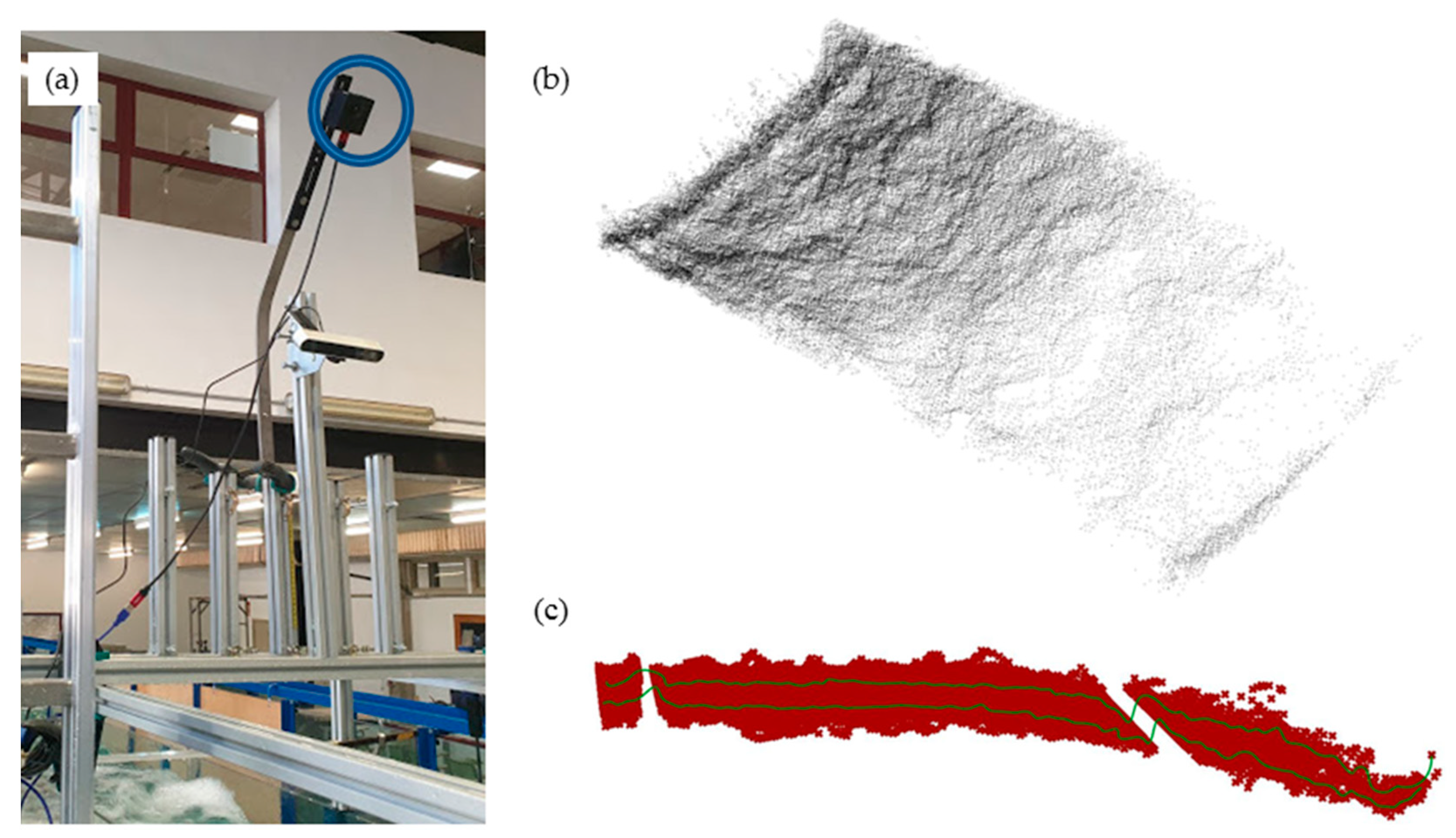
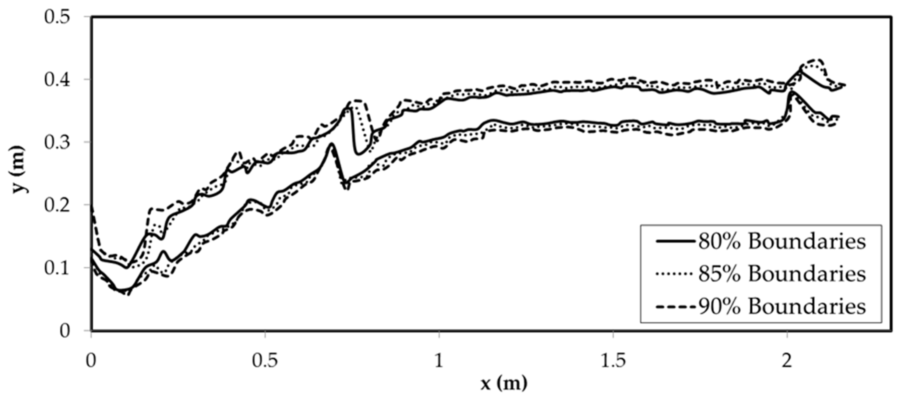
Regarding the hydraulic jump free surface, the first step was to process the data collected with the time-of-flight camera. To this end, anomalous values and outliers caused by splashing and droplets were discarded. This made it possible to obtain a series of bands containing a specific percentage of the measured points along the hydraulic jump longitudinal axis during the data collection time. Figure 5 shows the lower and upper boundaries for the bands containing 80%, 85% and 90% of the measured points.

The bands displayed in Figure 5 show that there are very slight differences, regardless of the percentage of measured points taken to create the band. This fact gives an indication of the results’ consistency after using LIDAR techniques for the characterization of the free surface profile in the hydraulic jump. Moreover, the observed differences between the lower and the upper boundaries of the represented bands reflect an acceptable uncertainty of the technique employed, considering the intense free surface fluctuations occurring in a hydraulic jump. However, additional filtering was necessary to overcome certain limitations derived from the physical characteristics of the model and the positioning of the instrumentation. As observed in Figure 5, for the lowest x values (i.e., surroundings of the hydraulic jump toe in the beginning of the basin), the camera collected part of the free surface profile in the sloping channel. This data had to be discarded since it was part of the free surface profile upstream of the hydraulic jump toe. Moreover, for x~0.7 m and for x > 2 m, the structure of the channel interfered with the measurements. The interference was caused by the methacrylate crossbars used to reinforce the channel, which were placed between the hydraulic jump and the camera. Accordingly, these parts of the profile were substituted by discrete measurements using limnimeters.

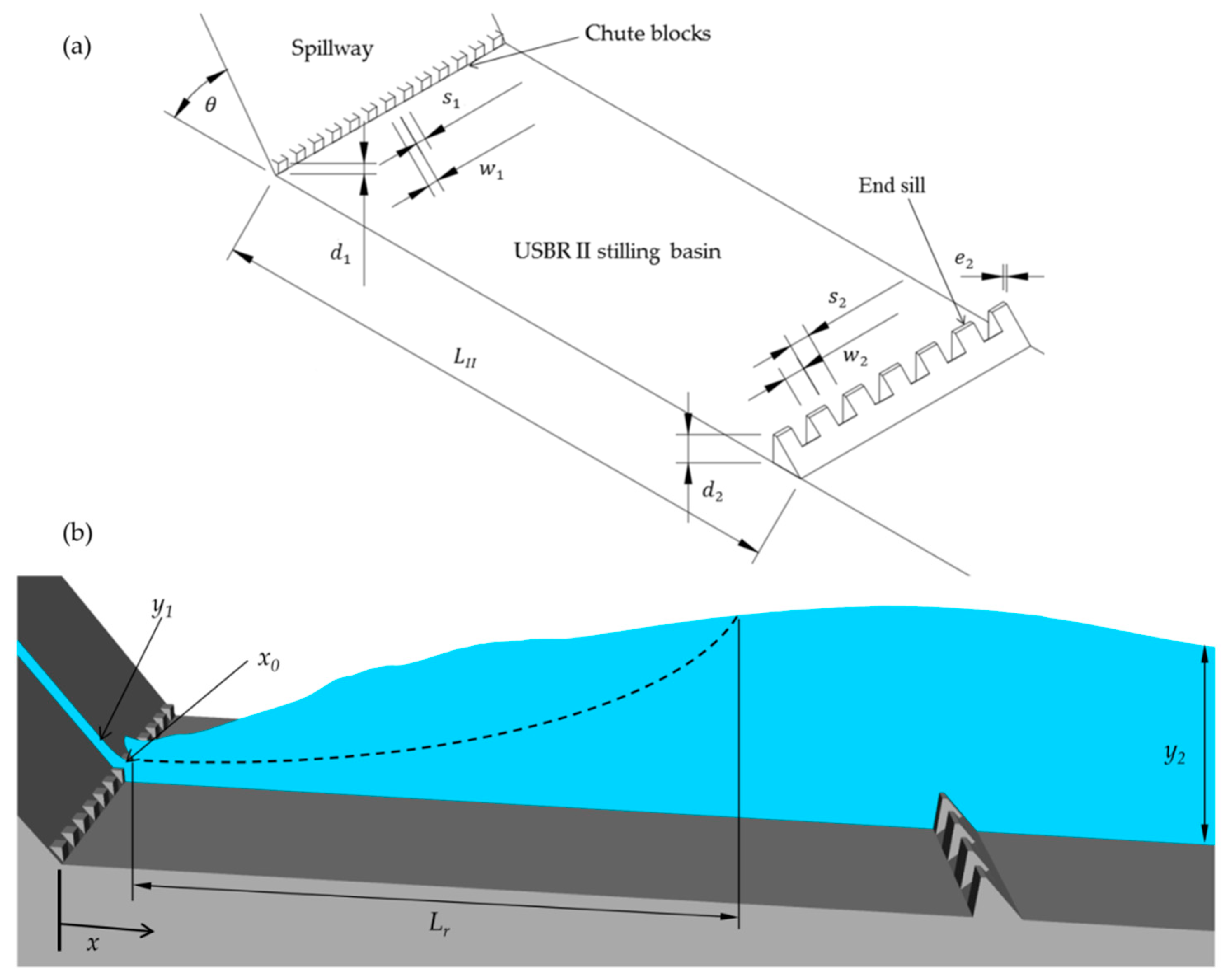
Finally, the information collected was employed to obtain the mean free surface profile along the physical model longitudinal axis. For convenient comparison with previous literature results, dimensionless values were calculated following the expressions proposed by Hager [2]:

$$X=\frac{x-x_0}{L_r}$$

(6)

$$Y=\frac{y-y_1}{y_2-y_1}$$

(7)

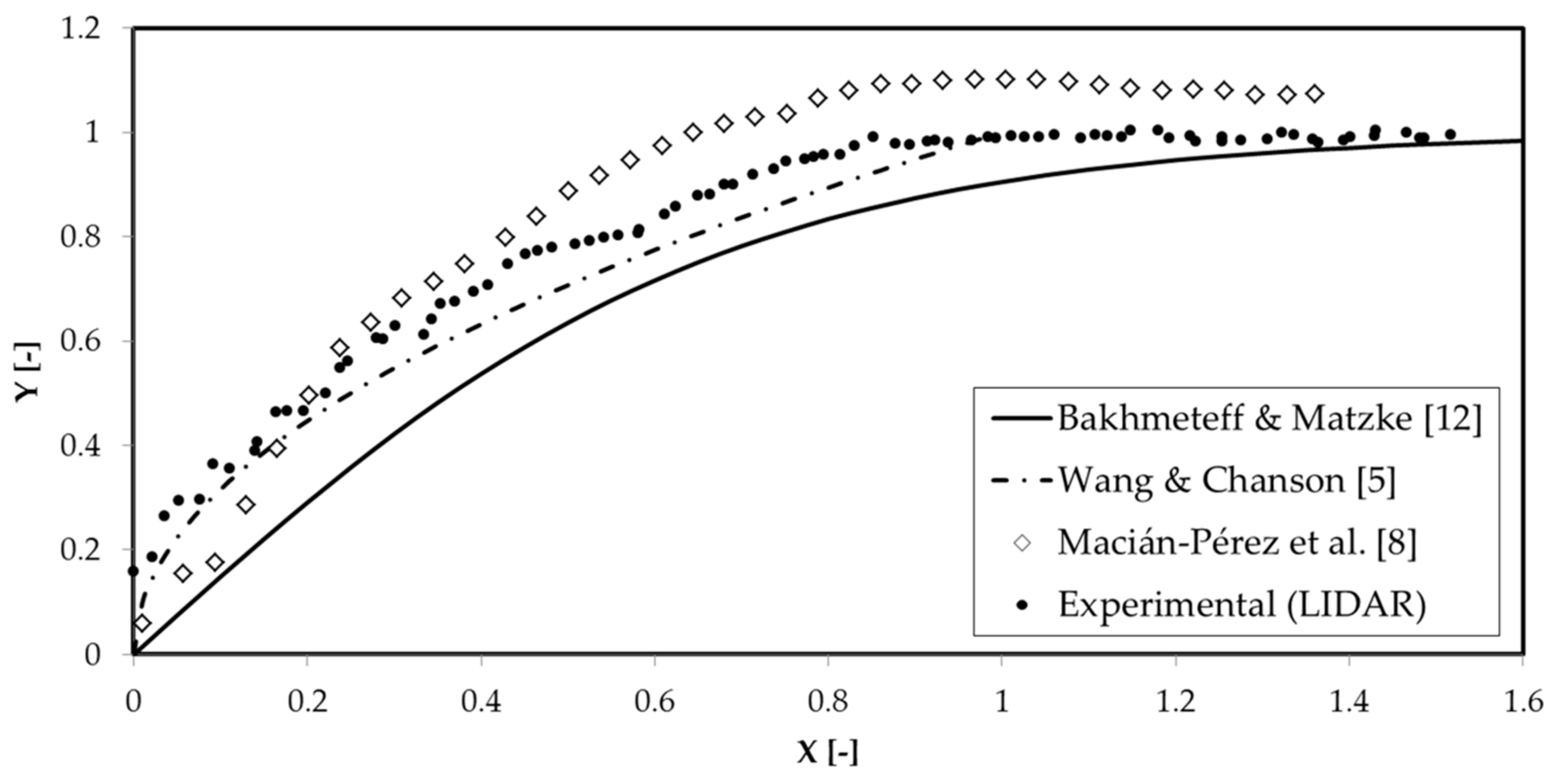
where $x_0$ is the hydraulic jump toe position and $L_r$ is the hydraulic jump roller length. The hydraulic jump roller length in the physical model was estimated from the velocity measurements performed with the Pitot tube, as developed in Section 3.3. The dimensionless free surface profile hence obtained is shown in Figure 6. These experimental results are compared to three different sources of bibliographic data [5,8,12].

A general observation of the results presented in Figure 6 shows that the physical model and the measuring techniques employed were able to provide a free surface profile in good agreement with previous studies. Nevertheless, some differences between profiles are to be discussed. It should be pointed out that Bakhmeteff & Matzke [12] and Wang and Chanson [5] profiles were originally obtained from the study of the CHJ. From this point of view, higher measured values of flow depth in the physical model should be expected, because of the effect of the energy dissipation devices on the flow profile. More specifically, the chute blocks placed at the beginning of the stilling basin model (X = 0) necessarily produce higher flow depths immediately downstream, when compared to those of a CHJ. As can be observed in Figure 6, such higher flow depths basically remain along the central part of the roller, up to X~0.9, where the profile seems to reach the subcritical flow depth. Thus, the subcritical flow depth was reached, in the stilling basin physical model, closer to the hydraulic jump toe, when compared to the CHJ, in which flow depths keep increasing at least up to X~1.5.

As stated by Hager [2], the energy dissipation devices in a typified USBR II stilling basin provide shorter hydraulic jumps. The results presented in Figure 6 help to quantify the effect of the energy dissipation devices on the hydraulic jump dimensions. Thus, they constitute an interesting step forward to characterize the hydraulic jump developed in stilling basins, although a wider range of inflow conditions should be tested to confirm the results.

This influence of the energy dissipation devices in the free surface profile was analyzed and discussed in Macián-Pérez et al. [8], also for a typified USBR II physical model. As shown in Figure 6, certain differences in non-dimensional depths are found between the present research and Macián-Pérez et al. [8]. For X > 0.2, the profile reported herein clearly lies below the one obtained in [8]. This behavior is probably explained by some limitations and particularities of the two different measurement methods used. As discussed in Macián-Pérez et al. [8], the Digital Image Processing (DIP) techniques used in that research tend to overestimate the depths of the free surface profile, mainly due to two factors. On the one hand, the intense aeration characteristic of the hydraulic jump phenomenon leads to bubbles and droplets being continuously expelled. This causes changes of light intensity that introduce bias in the image treatment. On the other hand, DIP techniques are based on images taken from the side of the experimental channel [30]. The time-of-flight camera used herein, though, allows a better estimation of the free surface profile along the longitudinal axis of the hydraulic jump.

Overall, the presented technique for determining the free surface profile seemed to overcome some limitations associated with other methodologies such as the DIP, but still reflects a clear influence of the energy dissipation devices in comparison with the results for the CHJ. Thus, the time-of-flight camera, based on LIDAR techniques, showed great potential to perform free surface profile measurements in aerated flows such as the hydraulic jump. Apart from the mentioned advantages in the results, the economic cost and the time consumed by LIDAR techniques is competitive when compared to the bibliographic methodology analyzed. Furthermore, LIDAR techniques would make it possible to obtain information regarding the 3D free surface structure of the hydraulic jump. Consequently, the formation of oblique shock-waves and the interference of the channel sidewalls could be addressed [31,32]. This information is of utmost importance and should undoubtedly be considered in further research lines.

3.2. Hydraulic Jump Efficiency

The hydraulic jump efficiency ($\eta$) for the physical model was also calculated through the expression:

$$\eta =\frac{H_{01}-H_{02}}{H_{01}}$$

(8)

where $H_{01}$ and $H_{02}$ are the specific energy heads upstream and downstream of the hydraulic jump. This parameter is directly related to the energy loss in the hydraulic jump. Therefore, it is crucial in the design of stilling basins. These structures must adapt to new scenarios posed by climate change and societal demands regarding flood protection. Under these new scenarios, existing stilling basins must cope with larger discharges than those considered for their original design. Any modification conducted for the stilling basin adaptation must still guarantee the fulfillment of its energy dissipation purpose. Consequently, it is of utmost importance to analyze the efficiency of the hydraulic jump developed in stilling basins.

The hydraulic jump efficiency derived from the sequent depths ratio values obtained for CHJ was also computed through Equation (8). This allowed the comparison between efficiencies of the hydraulic jump in a typified USBR II stilling basin and the CHJ (

Table 4. Hydraulic jump efficiencies obtained in the physical model and with bibliographic expressions.

Source	$\mathbf{Hydraulic}\mathbf{Jump}\mathbf{Efficiency}\left(\mathit{\eta }\right)$
Experimental campaign	0.705
Bélanger [28]	0.696
Hager & Bremen [29]	0.701

).

Due to the close link between hydraulic jump efficiency and sequent depths ratio, Table 4’s results are consistent with those previously presented in Table 3. In fact, lower sequent depths ratios yielded higher efficiencies, as expected. Therefore, the efficiency of the hydraulic jump developed in the stilling basin is slightly higher than the efficiency of a CHJ, under the same conditions (Table 4). This higher efficiency reflects the main design purpose of the energy dissipation devices placed in the stilling basin. Padulano et al. [7], in their experimental study of a typified USBR II stilling basin, tested hydraulic jumps with a wide variety of inflow Froude numbers. These authors obtained efficiency values between 0.700 and 0.750 for hydraulic jumps with Fr₁~9, in good agreement with the results of the present research.

3.3. Hydraulic Jump Roller Length

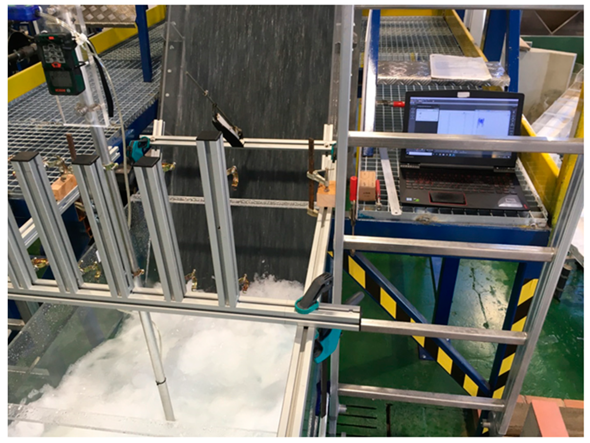
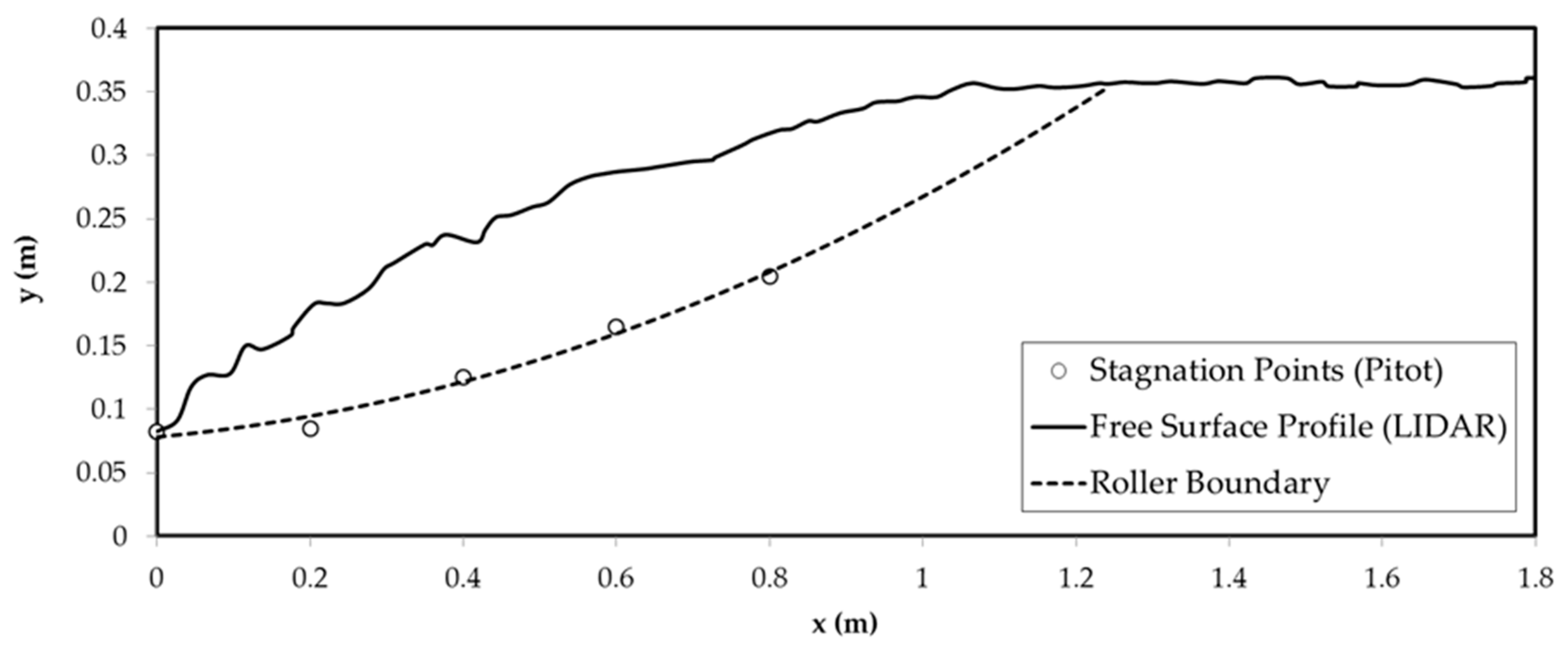
The hydraulic jump roller length was also estimated using the information collected in the experimental campaign. To this end, the stagnation point criterion was employed [33], taking the streamwise velocity vertical profiles measured in several sections throughout the hydraulic jump roller region. In each of these profiles, the point where velocity tended to zero, namely the stagnation point, was identified. The intersection between the line that joined all of the identified stagnation points and the averaged free surface profile led to the roller end section. With regard to the beginning of the hydraulic jump roller, it was directly located at the hydraulic jump toe (Figure 7). It is important to highlight the existence of intense fluctuations bound to the hydraulic jump nature that add uncertainty to the estimation of the roller length. Thus, there are fluctuations not only in the velocity field, but also in the free surface and the jump toe position. However, this criterion has proven to provide successful estimations of the parameter [4,33].

The hydraulic jump roller length estimated with the stagnation point criterion was L_r = 1.25 m. For comparison purposes, the roller length was also computed through the analytical expression presented by Hager et al. [33]:

$$\begin{array}{c}{L}_r=y_1\left[-12+160\tanh \left(\raisebox{1ex}{$F{r}_1$}\!\left/ \!\raisebox{-1ex}{$20$}\right.\right)\right] for \raisebox{1ex}{$y_1$}\!\left/ \!\raisebox{-1ex}{$b$}\right.<0.10\\ L_r=y_1\left[-12+100\tanh \left(\raisebox{1ex}{$F{r}_1$}\!\left/ \!\raisebox{-1ex}{$12.5$}\right.\right)\right] for 0.10<\raisebox{1ex}{$y_1$}\!\left/ \!\raisebox{-1ex}{$b$}\right.<0.70\end{array}$$

(9)

Using Equation (9), which was proposed for CHJ, the resulting roller length was L_r = 1.67 m. Thus, the physical model provided a considerably shorter roller region. This is in good agreement with the results presented in Figure 6 regarding the free surface profile of the hydraulic jump in the basin, which reached the subcritical depth faster than the CHJ. Accordingly, the results show that the stilling basin energy dissipation devices provide shorter hydraulic jump lengths, as previously stated by Hager [2]. A better understanding of how these devices shorten the hydraulic jump is essential for the improved design of stilling basins and their adaptation to larger discharges. Therefore, it is worth considering further research on the topic, involving different stilling basin geometries and inflow conditions, to identify characteristic trends and patterns in the hydraulic behavior of the structure.

The estimation of the hydraulic jump roller length could also be improved by using experimental techniques able to provide precise measurements of backwards velocities and in highly aerated areas, such as the optical-fibre probe or the Particle Image Velocimetry (PIV). However, the Pitot tube proved to be a low-cost alternative that leads to appropriate estimations of the roller length through the stagnation point criterion, in spite of its limitations.

3.4. Velocity Distribution

The velocity distribution of the flow developed in the stilling basin physical model was characterized. To do so, a series of streamwise velocity vertical profiles were measured along the longitudinal axis of the horizontal channel.

Table 5. Normalized position of the velocity profiles measured in the experimental campaign.

Vertical Profile	$\mathit{X}$1,2
V1	0.16
V2	0.32
V3	0.48
V4	0.64
V5	0.80
V6	0.96
V7	1.12

¹ The normalized position was obtained with Equation (6). ² End sill position: $X$ = 1.33.

shows the location of the different profiles considered to characterize the velocity field.

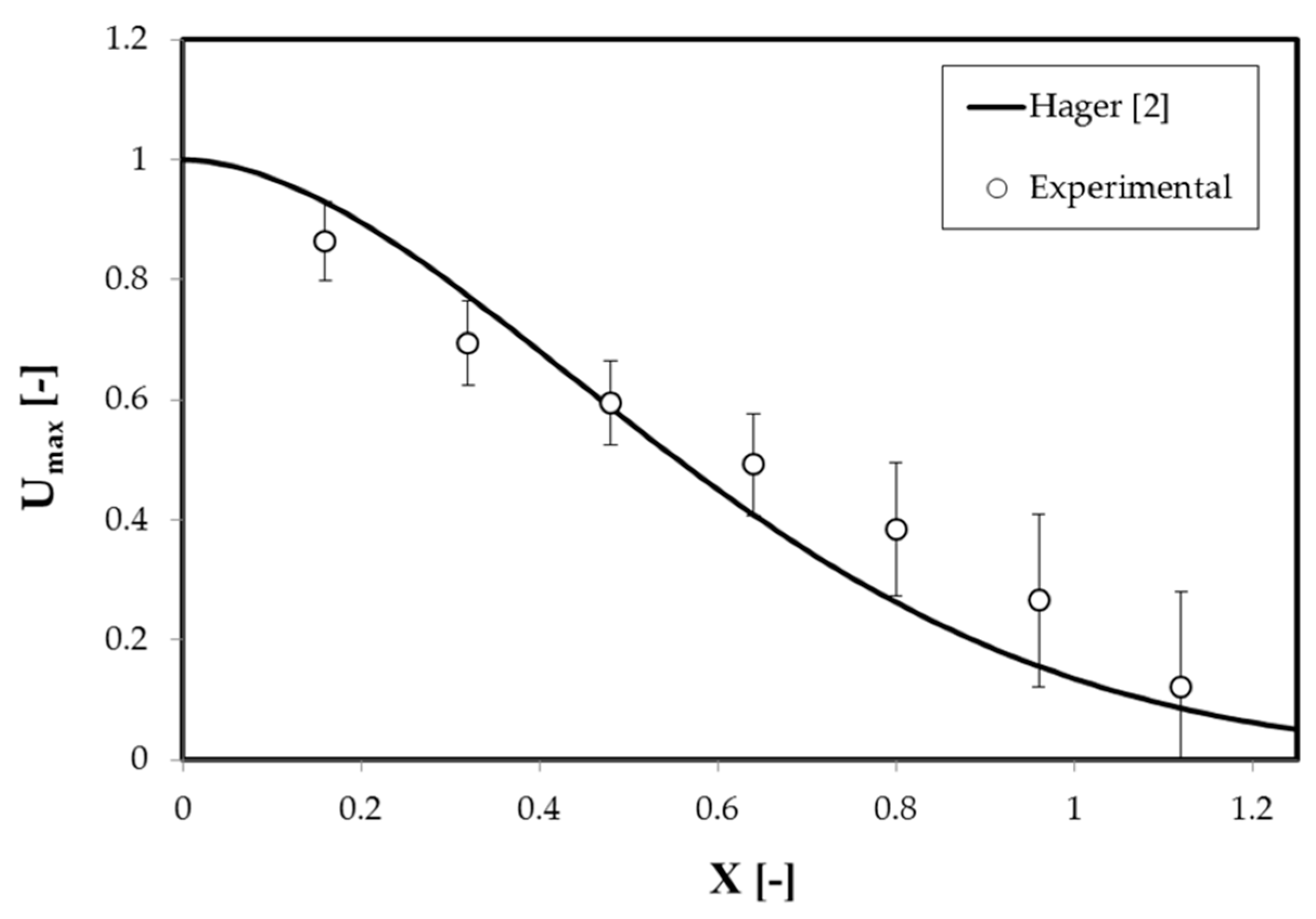
The first step in the analysis of the velocity distribution in the stilling basin model was focused on the maximum forward velocity decay. To this end, the expression proposed by Hager [2] for CHJ was compared with the experimental information collected in the model using the Pitot tube (Figure 8). The dimensionless value of the maximum velocity for each profile ($U_{max})$ was obtained with the following expression:

$$U_{max}=\frac{u_{max}-u_2}{u_1-u_2}$$

(10)

where $u_{max}$ is the maximum forward velocity value of the profile; $u_1$ and $u_2$ are, respectively, the depth-averaged velocities upstream and downstream the hydraulic jump.

The results displayed in Figure 8 show a good agreement between the maximum forward velocity decay obtained in the stilling basin physical model with the Pitot tube and the analytical expression for CHJ by Hager [2]. However, a slightly slower decay was observed for the experimental results. This implies that the differences in the maximum velocity values for profiles in different positions were not as large in the stilling basin model as for the CHJ. A possible explanation for this is the influence of the energy dissipation devices providing a more stable velocity distribution in terms of the longitudinal position.

Error bars were added in Figure 8 since considerable uncertainty in the velocity measurements along the hydraulic jump was expected. These bars show the uncertainty of each measurement using one standard deviation of the collected data for the corresponding point. Considering the strong velocity fluctuations in the hydraulic jump phenomenon [4,5], the Pitot tube provides an acceptable uncertainty, although an increase in the error bars can be observed as the measurements move downstream of the hydraulic jump toe.

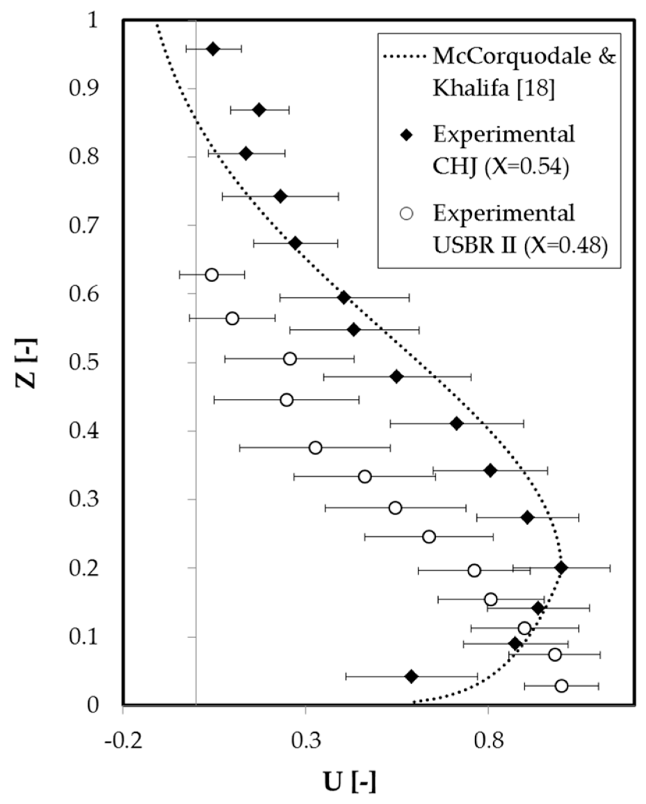
For the individual analysis of the complete profiles, in spite of the large number of points measured with the Pitot tube for each of them, the results provided a discrete and not a continuous velocity distribution. In addition, several tests conducted in the experimental channel, with the Pitot tube placed in a reverse position, showed that this device was not able to capture backwards velocities in the flow. A first attempt to overcome these issues was made by comparing the experimental data with the analytical expression for CHJ proposed by McCorquodale and Khalifa [18] (Figure 9). According to these authors, the mean vertical velocity distribution within the CHJ can be expressed through two functions:

$$u=u_{max}{\left(\frac{z}{\delta }\right)}^{1/7};0\le z\le \delta$$

(11)

$$u=u_{\infty }+u_t{e}^{2.772{\left(z-\delta /y-\delta \right)}^2} ; \delta <z<y$$

(12)

where $u$ is the horizontal velocity, which achieves its maximum value ($u_{max}$) at a height $z$ = $\delta$. In addition, $u_{\infty }$ is the horizontal component of the freestream velocity, defined by McCorquodale & Khalifa [18] as the velocity obtained for $z$→$\infty$. Finally, $u_t$ = $u_{max}$ − $u_{\infty }$. Figure 9 shows an example with one of the profiles measured in the physical model together with a profile in a CHJ, also measured with the Pitot tube, both for a similar position along the hydraulic jump. In order to represent together velocity profiles coming from different hydraulic jumps, the values were normalized as:

$$Z=\frac{z}{y}$$

(13)

$$U=\frac{u}{u_{max}}$$

(14)

where $y$ and $u_{max}$ are the flow depth and the maximum velocity, respectively, both in the corresponding vertical profile under study.

Figure 9 shows that the streamwise velocity vertical profiles for the hydraulic jump in the stilling basin differed from the typical shape for a CHJ and, therefore, it was not possible to adjust the analytical expression by McCorquodale and Khalifa [18]. The main differences are derived from the fact that, for the stilling basin model, the maximum velocity was located in the lowest part of the vertical profiles. In contrast, for the CHJ, there is an increase in the streamwise velocity values from the channel streambed, until the maximum velocity value is reached. This differences in the stilling basin were observed for profiles up to V4 ($X$ = 0.64), meaning that the maximum velocity was reached in the lowest part of the profile for a significant part of the hydraulic jump developed in the energy dissipation structure. As observed during the experimental campaign, the explanation arises from the effect of the chute blocks at the beginning of the basin. The deflection caused by these energy dissipation devices triggers the flow in the region next to the channel streambed and hence, the maximum velocities are achieved in the lowest part of the vertical profiles.

As previously mentioned, this effect was clearly noted for the three profiles closest to the beginning of the basin (V1–V3), whereas for the three next profiles (V4–V6) the maximum velocity did not correspond with the lowest measured position. As it was expected, the effect of the deflection caused by the chute blocks on the flow was lower for further positions and consequently, the differences between the profiles measured in the basin and the typical shape expected for a CHJ tended to decrease as the profile moved downstream. However, the influence of the energy dissipation devices on these profiles (V4–V6) was still observable through the low $\delta$ values obtained in comparison with the CHJ. Finally, the profile V7 was located downstream of the hydraulic jump roller. Consequently, the analytical expression for velocity profiles in the roller region of a CHJ (Equations (11) and (12)) was not strictly followed by this profile. Thus, the discussed discrepancies prevent the adjustment of the analytical profile by McCorquodale and Khalifa [18] to the values measured in the stilling basin physical model. In addition to this, the limitations of the instrumentation to measure backwards velocities in the hydraulic jump flow discarded the possibility of obtaining continuous velocity profiles.

The uncertainty of the measurements performed to achieve the streamwise velocity vertical profiles was also considered through the error bars included in Figure 9. The hydraulic jump is characterized by intense velocity fluctuations [4,5], which are clearly reflected in the uncertainties obtained. It is important to highlight that no significant differences were found between the error bars obtained for the CHJ and the hydraulic jump in the typified USBR II stilling basin.

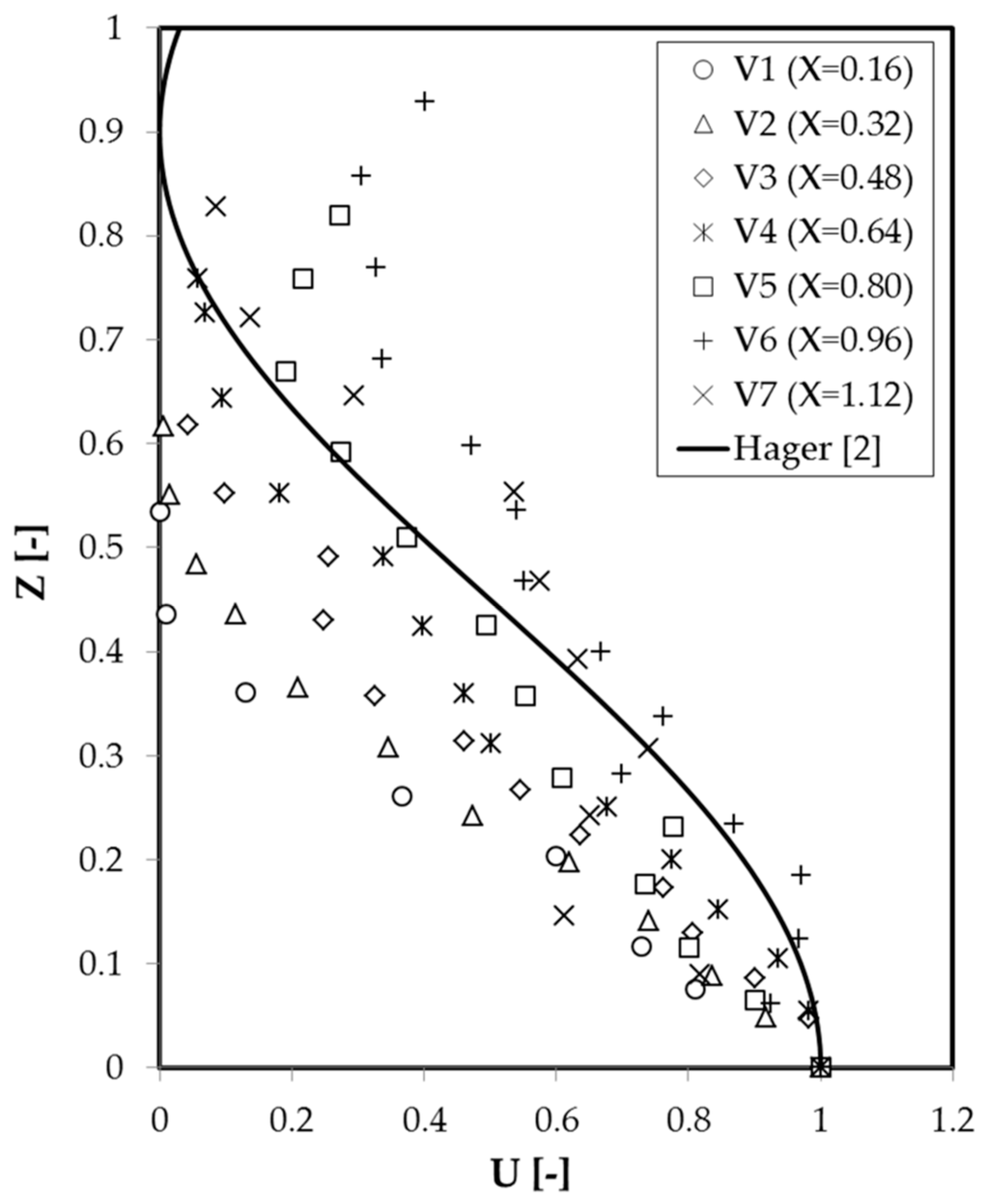
Despite the mentioned difficulties, further comparison of the measured profiles was conducted to gain a better insight into the influence of the energy dissipation devices on the velocity distribution. The profiles were represented together with the expression proposed by Hager [2] for the diffusion portion of velocity profiles in the CHJ roller region (Figure 10):

$$U={\left[\cos \left(100Z\right)\right]}^2$$

(15)

where $U$ is the dimensionless velocity and $Z$ is the dimensionless position in the vertical profile. These dimensionless values were obtained through the following procedure, also proposed by Hager [2]:

$$Z=\frac{z-\delta }{y-\delta }$$

(16)

$$U=\frac{u-u_s}{u_{max}-u_s}$$

(17)

where, for each vertical profile, $z$ is the measured position; $y$ is the flow depth; $u_{max}$ and $u_s$ are, respectively, the maximum velocity and the maximum backwards velocity; $\delta$ is the position at which $u$ = $u_{max}$.

The observation of Figure 10 shows significant differences among the experimental velocity profiles measured in the stilling basin model. Differences are also found in comparison with the theoretical expression for CHJ proposed by Hager [2]. In general, as shown in Figure 10, the observed differences tend to increase for higher $Z$ values, associated with a larger presence of bubbles. This fact has a feasible explanation by considering the difficulties of the Pitot tube to take reliable measurements in highly aerated regions with intense velocity fluctuations, such as the hydraulic jump recirculating region [22,27]. As previously explained, these limitations could not be addressed by the adjustment of an analytical expression such as the one presented by McCorquodale and Khalifa [18]. Consequently, the backwards velocities could not be properly estimated, which significantly affected the accuracy of the dimensionless representations derived from Equations (16) and (17).

However, in spite of the limitations of the measuring instrumentation employed, some interesting results were observed. Firstly, the velocity decay from the channel streambed was faster in the measured profiles when compared to the analytical expression for a CHJ (Equation (13)). As can be observed, almost every experimental profile shows lower velocity values than the expression by Hager [2], especially for low $Z$ values. A possible explanation for this is the previously observed effect of the energy dissipation devices. The deflection of the flow caused by these devices led to the maximum velocity values taking place in the lowest part of the profile. From this maximum value, very close to the streambed, the measured velocity decay is steeper than the one for the CHJ, probably because the acceleration of the flow caused by the deflection only affects the flow area adjacent to the channel streambed. In fact, this faster decay is more relevant in the profiles closer to the chute blocks (V1–V3), supporting the explanation based on the influence of the energy dissipation devices on the flow.

In these terms, as the velocity profiles moved downstream from the beginning of the basin (V4 and V5), the differences decreased and they tended to approach the CHJ velocity profile (Equation (13)). Again, this was in good agreement with the chute blocks causing the main differences between the velocity profiles measured in the stilling basin model and the typical shape for a CHJ velocity profile. Concerning velocity profiles V6 and V7, they were located in the surroundings of the roller end position ($X$ = 1). Therefore, a higher variability was observed and the trend established for velocity profiles in the roller region could not be strictly followed. However, these profiles are still influenced by the hydraulic jump flow and also by the presence of the end sill ($X$~1.30). Consequently, the profiles neither followed a velocity distribution for subcritical flow in open channels like the one presented by Kirkgoz and Ardiclioglu [34].

To sum up, the measurements performed in the stilling basin physical model with the Pitot tube present some limitations, which have been discussed. In spite of this, the experimental campaign made it possible to shed light on some features of the velocity distribution within the hydraulic jump developed in the typified USBR II stilling basin. In particular, it was clearly shown that the maximum forward velocity presented slighter differences among the profiles in relation with their position along the jump, when compared with the CHJ. Furthermore, the flow deflection caused by the chute blocks in the beginning of the basin provided the highest velocity values in the lowest region of the flow, for profiles within the first half of the roller region. For downstream profiles, the effect was reduced but still noted. Finally, for profiles close to the end of the roller region, it was difficult to identify a defined trend, since the influence of the end sill joined the location of these profiles in the boundary between the hydraulic jump roller and the subcritical flow. Overall, the Pitot tube constitutes a low-cost alternative to more sophisticated techniques such as the optical-fibre probes or the PIV. This device was able to provide useful information regarding the performance of the model and has proven to deal better with bubbles and high velocities than other devices tested, like the Acoustic Doppler Velocimeter (ADV).

4. Conclusions

The adaptation of existing stilling basins to larger discharges than those considered in their design constitutes a challenge of utmost importance in hydraulic engineering. The urgency to undertake this adaptation is constantly increasing due to the new scenarios posed by climate change effects and flood protection requirements. In order to approach the adaptation process, it is crucial to expand the knowledge regarding the phenomenon used for energy dissipation purposes in stilling basins, namely the hydraulic jump. The complexity of this phenomenon makes physical modeling essential for the study of stilling basins.

In these terms, a typified USBR II stilling basin physical model was developed to characterize the free surface profile and the velocity distribution in the associated hydraulic jump, through the corresponding experimental campaign. The design of the physical model was carefully developed as different factors were involved. Firstly, a representative case study with general interest in the hydraulic engineering field was chosen. In addition, the flow conditions and dimensions of the model had to consider not only the available resources in the laboratory, but also the guidelines and recommendations to avoid significant scale effects. The final design was a compromise solution among all of these factors.

Once the physical model was set, the results obtained in the experimental campaign were compared with bibliographic data and analytical expressions. This comparison was aimed at addressing different objectives. On the one hand, the suitability of the employed instrumentation was assessed. The complexity of the phenomenon under study brings the importance of using a varied methodology into the spotlight. Consequently, the performance of both traditional and innovative techniques must be approached. On the other hand, the free surface profile and the velocity distribution within the hydraulic jump developed in the model were analyzed. The results were also compared with data coming from the study of the CHJ, to gain a better understanding of the effect of the energy dissipation devices on the flow.

In particular, the results measured with the time-of-flight camera, based on LIDAR technology, showed great potential for the device, as an innovative technique in hydraulic engineering. The free surface profile obtained with this instrumentation was able to overcome the issues associated with other techniques traditionally employed, such as digital image processing. Furthermore, the influence of the energy dissipation devices was clearly identified in the presented results. The free surface profile measured in the stilling basin model showed a shorter hydraulic jump with higher flow depths close to the jump toe, in comparison with the CHJ. The sequent depths ratio and the hydraulic jump efficiency resulting from these measurements also revealed the energy-dissipating purpose of the stilling basin, in good agreement with previous research on the topic.

Regarding the velocity distribution, the research confirmed the limitations of the Pitot tube to obtain reliable data in certain regions of the hydraulic jump, where there is a higher density of air bubbles. However, some interesting results were achieved, showing that this instrumentation is able to provide useful information to characterize the velocity distribution within a hydraulic jump. Thus, the Pitot tube constitutes a low-cost alternative to more expensive techniques such as optical-fibre probes or the PIV, and proved to be more reliable than ADV for hydraulic jump measurements. In particular, the maximum forward velocity decay was successfully represented in the model. Moreover, the analysis of the streamwise velocity vertical profiles showed the flow deflection caused by the chute blocks at the beginning of the basin. This feature led to profiles with the maximum velocity value in their lowest part for the first half of the roller region, in contrast with the theoretical velocity profiles expected for a CHJ. The results presented, both for the free surface profile and the velocity distribution, are expected to extend the relatively few sources of comparison available for the study of stilling basins with energy dissipation devices.

Overall, this research shows the design process of a hydraulic engineering physical model, through a series of unavoidable steps. The resulting model, together with the experimental campaign carried out, provided a successful representation of the free surface profile and the velocity distribution within the hydraulic jump. However, the available laboratory resources prevented the testing of further experimental conditions, which would undoubtedly improve and complement the presented results. Therefore, further research lines should consider different discharges and a wider range of inflow Froude numbers.

Despite the discussed limitations, the results obtained shed light on the use of both new and traditional experimental instrumentation to collect information on complex hydraulic phenomena. The research also contributes to the characterization of the hydraulic jump developed in a typified USBR II stilling basin. These results can in turn be used to face hydraulic engineering challenges posed by climate change, such as the adaptation of existing stilling basins.

References

1. Vischer, D.L.; Hager, W.H. Dam Hydraulics; JOHN WILEY SONS: Chichester, UK, 1998. [Google Scholar]
2. Hager, W.H. Energy Dissipators and Hydraulic Jump; Springer Science & Business Media: Dordrecht, The Netherlands, 1992. [Google Scholar]
3. Valero, D.; Viti, N.; Gualtieri, C. Numerical Simulation of Hydraulic Jumps. Part 1: Experimental Data for Modelling Performance Assessment. Water 2019, 11, 36. [Google Scholar] [CrossRef] [Green Version]
4. Bayon, A.; Valero, D.; García-Bartual, R.; Vallés-Morán, F.J.; López-Jiménez, P.A. Performance assessment of OpenFOAM and FLOW-3D in the numerical modeling of a low Reynolds number hydraulic jump. Environ. Model. Softw. 2016, 80, 322–335. [Google Scholar] [CrossRef]
5. Wang, H.; Chanson, H. Experimental Study of Turbulent Fluctuations in Hydraulic Jumps. J. Hydraul. Eng. 2015, 141, 04015010. [Google Scholar] [CrossRef] [Green Version]
6. Fecarotta, O.; Carravetta, A.; Del Giudice, G.; Padulano, R.; Brasca, A.; Pontillo, M. Experimental results on the physical model of an USBR type II stilling basin. In Proceedings of the Riverflow 2016—8th International Conference on Fluvial Hydraulics, St. Louis, MO, USA, 12–15 July 2016. [Google Scholar]
7. Padulano, R.; Fecarotta, O.; Del Giudice, G.; Carravetta, A. Hydraulic design of a USBR Type II stilling basin. J. Irrig. Drain. Eng. 2017, 143, 04017001. [Google Scholar] [CrossRef] [Green Version]
8. Macián-Pérez, J.F.; García-Bartual, R.; Huber, B.; Bayón, A.; Vallés-Morán, F.J. Analysis of the Flow in a Typified USBR II Stilling Basin through a Numerical and Physical Modeling Approach. Water 2020, 12, 227. [Google Scholar] [CrossRef] [Green Version]
9. Montes, J.S.; Chanson, H. Characteristics of undular hydraulic jumps: Experiments and analysis. J. Hydraul. Eng. 1998, 124, 192–205. [Google Scholar] [CrossRef] [Green Version]
10. Ohtsu, I.; Yasuda, Y.; Gotoh, H. Hydraulic condition for undular-jump formations. J. Hydraul. Res. 2001, 39, 203–209. [Google Scholar] [CrossRef]
11. Ohtsu, I.; Yasuda, Y.; Gotoh, H. Flow conditions of undular hydraulic jumps in horizontal rectangular channels. J. Hydraul. Eng. 2003, 129, 948–955. [Google Scholar] [CrossRef]
12. Bakhmeteff, B.A.; Matzke, A.E. The Hydraulic Jump In Terms of Dynamic Similarity. Trans. Am. Soc. Civ. Eng. 1935, 101, 630–647. [Google Scholar]
13. Chachereau, Y.; Chanson, H. Free-surface fluctuations and turbulence in hydraulic jumps. Exp. Therm. Fluid Sci. 2011, 35, 896–909. [Google Scholar] [CrossRef] [Green Version]
14. Zhang, G.; Wang, H.; Chanson, H. Turbulence and aeration in hydraulic jumps: Free-surface fluctuation and integral turbulent scale measurements. Environ. Fluid Mech. 2013, 13, 189–204. [Google Scholar] [CrossRef]
15. Montano, L.; Li, R.; Felder, S. Continuous measurements of time-varying free-surface profiles in aerated hydraulic jumps with a LIDAR. Exp. Therm. Fluid Sci. 2018, 93, 379–397. [Google Scholar] [CrossRef]
16. Montano, L.; Felder, S. LIDAR Observations of Free-Surface Time and Length Scales in Hydraulic Jumps. J. Hydraul. Eng. 2020, 146, 04020007. [Google Scholar] [CrossRef]
17. Rajaratnam, N. The hydraulic jump as a well jet. J. Hydraul. Div. 1965, 91, 107–132. [Google Scholar]
18. McCorquodale, J.A.; Khalifa, A. Internal flow in hydraulic jumps. J. Hydraul. Eng. 1983, 109, 684–701. [Google Scholar] [CrossRef]
19. Tajabadi, F.; Jabbari, E.; Sarkardeh, H. Hydrodynamic analysis of flow in USBR stilling basin types I, II, III. J. Dam Hydroelectr. Powerpl. 2017, 4, 43–54. [Google Scholar]
20. Viti, N.; Valero, D.; Gualtieri, C. Numerical Simulation of Hydraulic Jumps. Part 2: Recent Results and Future Outlook. Water 2019, 11, 28. [Google Scholar] [CrossRef] [Green Version]
21. Blocken, B.; Gualtieri, C. Ten iterative steps for model development and evaluation applied to Computational Fluid Dynamics for Environmental Fluid Mechanics. Environ. Model. Softw. 2012, 33, 1–22. [Google Scholar] [CrossRef]
22. Carrillo, J.M.; Castillo, L.G.; Marco, F.; García, J.T. Experimental and numerical analysis of two-phase flows in plunge pools. J. Hydraul. Eng. 2020, 146, 04020044. [Google Scholar] [CrossRef] [Green Version]
23. Peterka, A.J. Hydraulic Design of Stilling Basins and Energy Dissipators; Department of the Interior, Bureau of Reclamation: Washington, DC, USA, 1978.
24. Chitale, S.V. Energy Dissipation in Hydraulic Jump below Weirs and Falls. Water Energy Int. 1959, 16, 465–477. [Google Scholar]
25. Heller, V. Scale effects in physical hydraulic engineering models. J. Hydraul. Res. 2011, 49, 293–306. [Google Scholar] [CrossRef]
26. Chanson, H. Bubble entrainment, spray and splashing at hydraulic jumps. J. Zhejiang Univ. A 2006, 7, 1396–1405. [Google Scholar] [CrossRef] [Green Version]
27. Wang, H. Turbulence and Air Entrainment in Hydraulic Jumps. Ph.D. Thesis, The University of Queensland, Brisbane, Australia, 2014. [Google Scholar]
28. Bélanger, J.B. Notes sur l’Hydraulique; Ec. R. des Ponts Chaussées: Paris, France, 1841. [Google Scholar]
29. Hager, W.H.; Bremen, R. Classical hydraulic jump: Sequent depths. J. Hydraul. Res. 1989, 27, 565–585. [Google Scholar] [CrossRef]
30. Bayón, A.; Macián-Pérez, J.F.; Vallés-Morán, F.J.; López-Jiménez, P.A. Effect of RANS turbulence model in hydraulic jump CFD simulations. In Proceedings of the 38th IAHR World Congress, Panama City, Panama, 1–6 September 2019. [Google Scholar]
31. Ben Meftah, M.; De Serio, F.; Mossa, M.; Pollio, A. Experimental study of recirculating flows generated by lateral shock waves in very large channels. Environ. Fluid Mech. 2008, 8, 215–238. [Google Scholar] [CrossRef]
32. Ben Meftah, M.; Mossa, M.; Pollio, A. Considerations on shock wave/boundary layer interaction in undular hydraulic jumps in horizontal channels with a very high aspect ratio. Eur. J. Mech. 2010, 29, 415–429. [Google Scholar] [CrossRef]
33. Hager, W.H.; Bremen, R.; Kawagoshi, N. Classical hydraulic jump: Length of roller. J. Hydraul. Res. 1990, 28, 591–608. [Google Scholar] [CrossRef]
34. Kirkgöz, M.S.; Ardiçlioğlu, M. Velocity profiles of developing and developed open channel flow. J. Hydraul. Eng. 1997, 123, 1099–1105. [Google Scholar] [CrossRef]
Figure 1. Design of the typified United States Bureau of Reclamation (USBR) II stilling basin physical model (flow from left to right): (a) Stilling basin including the design parameters: d1, w1 and s1 are the height, width and spacing of the chute blocks, whereas d2, w2 and s2 are these same values but for the blocks in the end sill. LII is the length of the basin, e2 is the width of the end sill top face and θ is the angle formed with the slopping channel; (b) sketch of the hydraulic jump along the stilling basin longitudinal axis.
Water 12 01758 g001
Figure 2. Physical model of the typified USBR II stilling basin built at the UPV Hydraulics Laboratory (Valencia, Spain).
Water 12 01758 g002
Figure 3. Light detection and ranging (LIDAR) techniques in the physical model (flow from right to left): (a) Time-of-flight camera placed in the experimental device; (b) point cloud obtained from the hydraulic jump free surface; (c) band containing 80% of the measured points.
Water 12 01758 g003
Figure 4. Pitot tube measures in the stilling basin physical model.
Water 12 01758 g004
Figure 5. Bands containing the 80%, 85% and 90% of the points measured along the hydraulic jump longitudinal axis with LIDAR technology.
Water 12 01758 g005
Figure 6. Dimensionless free surface profile of the hydraulic jump obtained from the physical model and comparison with bibliographic information [5,8,12].
Water 12 01758 g006
Figure 7. Stagnation point criterion to estimate the hydraulic jump roller length.
Water 12 01758 g007
Figure 8. Maximum forward velocity decay along the hydraulic jump longitudinal axis.
Water 12 01758 g008
Figure 9. Streamwise velocity vertical profiles in the hydraulic jump for X ~0.5 and adjustment of the analytical expression for Classical Hydraulic Jumps (CHJ) by McCorquodale and Khalifa [18].
Water 12 01758 g009
Figure 10. Velocity profiles along the longitudinal axis in the stilling basin physical model hydraulic jump.
Water 12 01758 g010