Do CFSv2 Seasonal Forecasts Help Improve the Forecast of Meteorological Drought over Mainland China?


1
School of Earth Sciences, Yunnan University, Kunming 650050, China
2
Department of Geography, Environment, and Spatial Sciences, Michigan State University, East Lansing, MI 48824, USA
3
Center for Global Change and Earth Observations, Michigan State University, East Lansing, MI 48824, USA
4
Faculty of Geographical Science, Beijing Normal University, Beijing 100875, China
5
College of Hydrology and Water resources, Hohai University, Nanjing 210098, China
*
Author to whom correspondence should be addressed.
Water 2020, 12(7), 2010; https://0-doi-org.brum.beds.ac.uk/10.3390/w12072010
Submission received: 2 June 2020
/
Revised: 8 July 2020
/
Accepted: 11 July 2020
/
Published: 15 July 2020
(This article belongs to the Special Issue Recent Advance in Drought Risk Assessment, Monitoring, and Forecasting)
Abstract
:Seasonal forecasts from dynamical models are expected to be useful for drought predictions in many regions. This study investigated the usefulness of the Climate Forecast System version 2 (CFSv2) in improving meteorological drought prediction in China based on its 25-year reforecast. The six-month standard precipitation index (SPI6) was used as the drought indicator, and its persistence forecast served as the benchmark against which CFSv2 forecasts were evaluated. The analysis found that the SPI6 persistence forecast shows good skills in all regions at short lead times, and CFSv2 forecast can further improve those skills in most regions. The improvement is particularly pronounced at longer lead times and over the humid regions in the southeast. This study also examined the seasonality and regionality of persistence forecast skills and CFSv2 contributions, and reveals regions where CFSv2 forecast shows no or sometimes even negative contributions.
1. Introduction
Drought is a major type of natural hazard in China that has historically affected many parts of the country. Some regions have experienced frequent and long-lasting droughts, which had significant impacts on agriculture, water resources, and socioeconomic activities. On average, about 19 million hectares of land are affected by drought annually, and the associated economic losses are about 70 billion RMB Yuan, according to China Civil Affairs’ Statistical Yearbook [1]. To minimize the losses and mitigate drought impacts, it is essential to establish a drought early warning system based on accurate drought monitoring and skillful seasonal drought prediction.
There are different types of droughts defined using different variables in the hydrological cycle (e.g., meteorological drought, agricultural drought, and hydrological drought), but most of them start with a prolonged precipitation deficiency with respect to the climatology. To quantify the precipitation anomaly and make it comparable across geographical locations and seasons, the standard precipitation index (SPI, [2]) was developed and has been widely used as an indicator for meteorological drought. SPI integrates precipitation variability over some time period (1, 3, 6, 12 months or more) and this cumulative, time-integrated nature results in considerable persistence from one month to the next, which gives SPI some predictable persistence characteristics. The persistence characteristics [3] are seen to drop off in a linear fashion with time lag, reaching a value of roughly zero when the time lag exceeds the accumulation period of the index. For example, the persistence characteristics of the SPI3 reach zero at a three-month lead time, and for the SPI6 reaches zero at a six-month lead time, and so on. These persistence characteristics of SPI are modulated by a region’s seasonal cycle of precipitation and its inter-annual variability. When SPI is used for drought forecasting, the accumulation period includes both observation and forecast. For a given combined three-, six-, or twelve-month period for total precipitation, the forecast skill is enhanced (reduced) when the variance of the forecast portion decreases (increases) relative to the variance of prior observational precipitation [3]. Thus the drought forecast skill from the persistence characteristics exhibits strong seasonality as well as regionality.
Owing to the predictable persistence characteristics, multi-month SPIs can be potentially used for drought early warning. Additionally, when combining precipitation observations in the recent past and forecast for the following months, the forecast skills of multi-month SPIs are expected to improve. For example, Quan et al. [4] combined prior observational precipitation with target season forecasts from the coupled climate forecast system (CFS) or the uncoupled global forecast system (GFS), and showed improved forecast skills relative to the unconditioned persistence forecasts over the US Great Plains. Dutra et al. [5] and Dutra et al. [6] developed an integrated drought monitoring and forecasting system by combining monthly precipitation monitoring products with six lead times of forecasts from the European Centre for Medium-Range Weather Forecasts (ECMWF) seasonal forecasting system, and showed that dynamic forecasts of precipitation provide added values to seasonal drought prediction.
With enhanced skills in dynamical seasonal prediction systems such as the Climate Forecast System version 2 (CFSv2) [7] from the National Centers for Environmental Prediction (NCEP), ENSEMBLES from the ECMWF [8], and North American Multimodel Ensemble (NMME) [9], seasonal drought prediction is expected to improve when model forecasts are properly used. Additionally, seasonal hydrological prediction driven by climate model forecast also becomes feasible [10,11,12,13,14,15]. In order to advance the seasonal hydrological and drought prediction capability in China, it is critical to identify the strength and weakness in the dynamical seasonal forecast, and to understand the seasonality and regionality associated with their forecast skills.
Previous studies, such as Mo and Lyon [16], have tackled similar questions in the global domain, but regional-focused studies are still needed to provide more detailed analysis. In this study, we were interested in understanding how the seasonal precipitation forecast from the state-of-the-art climate models can be used to improve meteorological drought prediction in China. We focused on CFSv2, which is the current operational model for seasonal prediction at the NCEP and its forecasts are freely available. If we can identify the strength and weakness in its forecasts, we can better utilize its forecast to provide more skillful and reliable early drought warnings. The CFSv2 reforecast and real-time forecast were evaluated in a number of studies over various regions (e.g., Yuan et al. [13], Kim et al. [17], Lang et al. [18], Luo and Zhang [19], Luo et al. [20], Mo et al. [21], Riddle et al. [22], Saha et al. [23], among others); however, the following questions remain unanswered and were addressed in this study: (1) how skillful the persistence forecast is for drought prediction in China; (2) how much improvement the CFSv2 forecast can contribute to the overall drought forecast skill; (3) how such improvements vary geographically and with season and lead time; (4) whether there are situations under which CFSv2 forecasts show no or even negative contributions to drought forecast skills.
2. Data and Method
The second version of the Climate Forecast System (CFSv2) became operational at the NCEP in March 2011. The CFSv2 [7] used in the reforecast consists of the NCEP Global Forecast System at T126 (∼0.937°) resolution, the Geophysical Fluid Dynamics Laboratory Modular Ocean Model version 4.0 at 0.25–0.5° grid spacing coupled with an interactive three layer sea-ice model, the four-layer NOAH land surface model, and historical prescribed (i.e., rising) concentrations. To provide a model climatology for better forecast calibration, a multi-year reforecast dataset was produced for the period of 1982 to 2009. The reforecast dataset includes four 9-month forecast runs at the 00, 06, 12, and 18 UTC cycles, a single one season (123-day) forecast run at the 00 UTC cycle, and 3 45-day forecast runs at the 06, 12, and 18 UTC cycles. The 9-month runs were initialized every 5 days starting from 1 January of each year due to constraint in computational resources. Monthly mean time series of precipitation from the 9-month forecast runs were obtained from the National Centers for Environmental Information (NCEI) for this study. All the forecast runs initialized between the 8th of a given month and the 7th of the following month were grouped as one ensemble. For example, forecasts initialized on January 11, January 16, January 21, January 26, January 31, and February 5 were grouped together to form the ensemble for February forecast. This results in an ensemble size of 24 for each month except for November, which has 28 forecast runs. The ensemble mean monthly total precipitation was used in this analysis, and the lead time spans between 0 and 9 months. All CFSv2 forecasts were regridded to the same 0.5° × 0.5° grid as the observational precipitation over East Asian domain. We used GrADS to do the spatial interpolation with a simple bilinear interpolation method.
The observational monthly precipitation data in this study were from the daily precipitation analysis developed by Xie et al. [24]. This dataset covers the East Asia domain (5–60° N, 65–155° E) at 0.5° × 0.5° resolution and spans over the period 1961 to 2007, and can be obtained from its web site (ftp://ftp.cpc.ncep.noaa.gov/precip/xie/EAG/EA_V0409). The use of observed precipitation was three fold. It was used to bias correct the model forecast as discussed below. The observation was then combined with the bias corrected forecast to construct a multi-month total precipitation for calculating the SPIs with different lead times. Finally, it was also used to evaluate both the persistence forecast and CFSv2 forecast. The evaluation was carried out over mainland China during the 25-year common period (i.e., 1982 to 2006) between the reforecast dataset and the observational dataset.
The six-month standard precipitation index (SPI6) [2] was used as the indicator for the medium-term meteorological drought and was computed following the method described in [25]. SPI6 values generally range between −3 and 3 with negative values indicating drier than normal conditions, and the magnitudes of the departure from zero is a probabilistic measure of the severity of a wet or dry event. Here, the construction of multiple lead-times SPI6 followed the procedures of Dutra et al. [26]. For a given 6-month target period, observations and forecast were concatenated in different lengths to create a combined 6-month total precipitation, which was then used to calculate the SPI6 for the period. For convenience, the SPI6 was always defined at the last month of the 6-month period. For example, September SPI6 was based on the total precipitation for April through September. The 1-month lead SPI6 for September was then based on the combination of observed precipitation for the first five months (April through August) and forecast for the last month (September). At the 6-month lead time, the SPI6 was based only on the precipitation forecast. Once the 6-month total precipitation was obtained for the target period, the SPI6 was calculated with respect to the observed climatological distribution for the period.
Because dynamic models like CFSv2 often have biases in their precipitation forecast, it is necessary to correct the precipitation bias before they are concatenated with observations to calculate the 6-month total precipitation. This is especially important when precipitation in the forecast portion of the 6-month period dominates, and thus, its bias can significantly distort SPI6 forecast skills. To remove the bias, a correction factor was calculated for each month as the ratio between the average of all observed precipitation and that of all CFSv2 forecast for the month. The bias correction is expressed as
where is the CFSv2 precipitation forecast at the month t, and and are the multi-annual mean of the historical observed precipitation and the CFSv2 forecast value for month t.
To determine if the CFSv2 forecasts help to improve drought prediction, a baseline SPI6 forecast is needed. Here, we take advantage of the persistence characteristics of SPI6, and fill the forecast portion of the 6-month total precipitation with the climatological mean precipitation. Thus, the baseline forecast skill only comes from the persistence of the precipitation anomaly in the observation portion. We denote this as persistence forecast, which is probably the best one can do when information on seasonal anomalies in future precipitation is absent. Using the persistence forecast as the benchmark, the usefulness of CFSv2 forecast can be quantified.
In this study, forecast skills were measured by the temporal anomaly correlation (TAC, or correlation) and root mean square error (RMSE), both of which were calculated for each grid and for all 6 lead times. The temporal anomaly correlation measures the degree of association between the forecast , either the CFSv2 forecast or the SPI6 persistence forecast, and the corresponding observed SPI6 at a given lead time (one- to six-month lead). It is computed as
where n is the total number of forecast, and are the climatological mean of observed and forecast SPI6. It is necessary to mention that the baseline persistence forecast of SPI6 at 6-month lead time consists of only the climatological mean, and the forecasts are the same for all 25 years for the same period, thus no correlation coefficient was calculated.
RMSE, on the other hand, measures the closeness of forecast and the corresponding observations of SPI6 over a time period, and is computed as
RMSE for a perfect forecast is zero, with a larger RMSE indicating a decreasing accuracy of the forecast.
With 25 years of CFSv2 reforecast, we obtained a total of 300 forecasts. We treated all these forecasts equally to calculate the overall correlation and RMSE, and we also stratified the forecasts by month (i.e., 25 forecast for each month) to obtain the metrics for each month. To make comparisons between CFSv2 forecast and persistence forecast, we also calculated the corresponding skill scores (Wilks [27]). Using persistence forecast as the reference forecast, the TAC skill score becomes
and the RMSE skill score (in proportion rather than percentage terms) becomes
where both skill scores range from minus infinity (no skill) to 1 (perfect forecast). A score larger than 0 indicates an improvement with respect to the persistence forecast, whereas a score smaller than 0 indicates that the CFSv2 forecast is inferior to the persistence forecast.
The ability of a forecast to reproduce the observed spatial patterns was examined with the spatial anomaly correlation (Murphy and Epstein [28], Krishnamurti et al. [29]). The spatial anomaly correlation (SAC) is a commonly used measure of association that operates on pairs of grid point values in the forecast and observed fields. The SAC is designed to detect similarities in the patterns of departures (i.e., anomalies) and is referred to as a pattern correlation. It is calculated as
where s denotes the corresponding grid point, m is the total number of grid points over the study domain, and are the spatial average of observed SPI6 over all grid points and the CFSv2 forecast or the persistence SPI6 forecast average of all grid points for a given time. indicts a perfect pattern correlation.
3. Results
We examined the skill of the persistence forecast first to provide the baseline. Figure 1 shows the overall skill of the persistence forecast at three different lead times. These were calculated based on all 300 forecasts during the 25-year period.
It is evident that the SPI6 persistence forecast was quite skillful everywhere in the domain at one-month lead time. The correlation coefficients (TAC) are above 0.8 and RMSE are mostly between 8 and 10. Over the humid regions in the southeast, the correlation coefficient is above 0.9. As lead time increases, the persistence forecast skill declines, expressed by the gradual decrease in correlation and the increase in RMSE. At the three-month lead time, some level of skill still exists over the entire domain with a correlation coefficient mostly above 0.5. Then at the five-month lead time, the skill continues to decline and the correlation coefficient is now around 0.3 to 0.4. At the six-month lead time (not shown), the persistence forecast skill completely diminishes simply because the forecast now only contains the climatological seasonal cycle, which has no skill for predicting anomalies. The values of RMSE may seem hard to interpret initially because they are based on SPI6 values, but when we compared the RMSE between different lead times in Figure 1, it becomes clear that RMSE is indeed much smaller at a shorter lead time. It is also worth emphasizing that the spatial patterns of skills measured by correlation and RMSE are very similar, as regions with higher correlation generally show smaller RMSE.
Figure 2 presents the difference in skill between the CFSv2 forecast and the persistence forecast. In the CFSv2 forecast, the bias-corrected CFSv2 precipitation forecast replaces the climatological mean precipitation in the forecast portion of the six-month total precipitation, the difference in forecast skills reflects the contribution of CFSv2 model to predicting meteorological droughts beyond the SPI6 persistence. At the one-month lead, while the persistence forecast establishes a high benchmark, the CFSv2 forecast shows marginally higher correlation and smaller RMSE over large areas. The only significant region where CFSv2 forecast consistently has a negative contribution is over the northwest arid region near Mongolia. These are desert regions where low amount of precipitation is received throughout a year with a small inter-annual variability, so it is difficult for CFSv2 forecast to add additional skills beyond the persistence forecast.
At longer lead times, as the CFSv2 precipitation forecast takes a bigger portion of the six-month total precipitation, the impact of CFSv2 forecast on the SPI6 forecast skill is expected to be greater. As shown in Figure 2, similar patterns of difference are observed but the difference is only more pronounced. The humid southeast generally shows larger increases in TAC especially at the five-month lead time. Reduction in RMSE also shows up in this region at all lead times. Over the semi-arid northwest, even larger decreases in correlation and increases in RMSE suggest a further degradation of skill in this region when CFSv2 forecast is included. Overall, CFSv2 forecast contributes positively to the skill of drought forecast with SPI6 over most regions in China at all lead times, mainly in northeast, southeast, and southwest of China, and the contribution is more significant at longer lead times.
Figure 3 further shows the skill scores of CFSv2 forecast with the persistence forecast as the reference at different lead times. Any positive values indicate that CFSv2 forecast is more skillful than the SPI6 persistence forecast. The patterns are the same as what is shown in Figure 2 for all lead times, but the magnitudes of improvement measured by skill score are different. For example, Figure 2a shows a small positive difference between CFSv2 forecast and the SPI6 persistence forecast. In Figure 3a, the skill score is much larger as the skill is already quite high in the reference forecast at one-month lead, even a small amount of improvement is quite significant. This is seen in both correlation and RMSE.
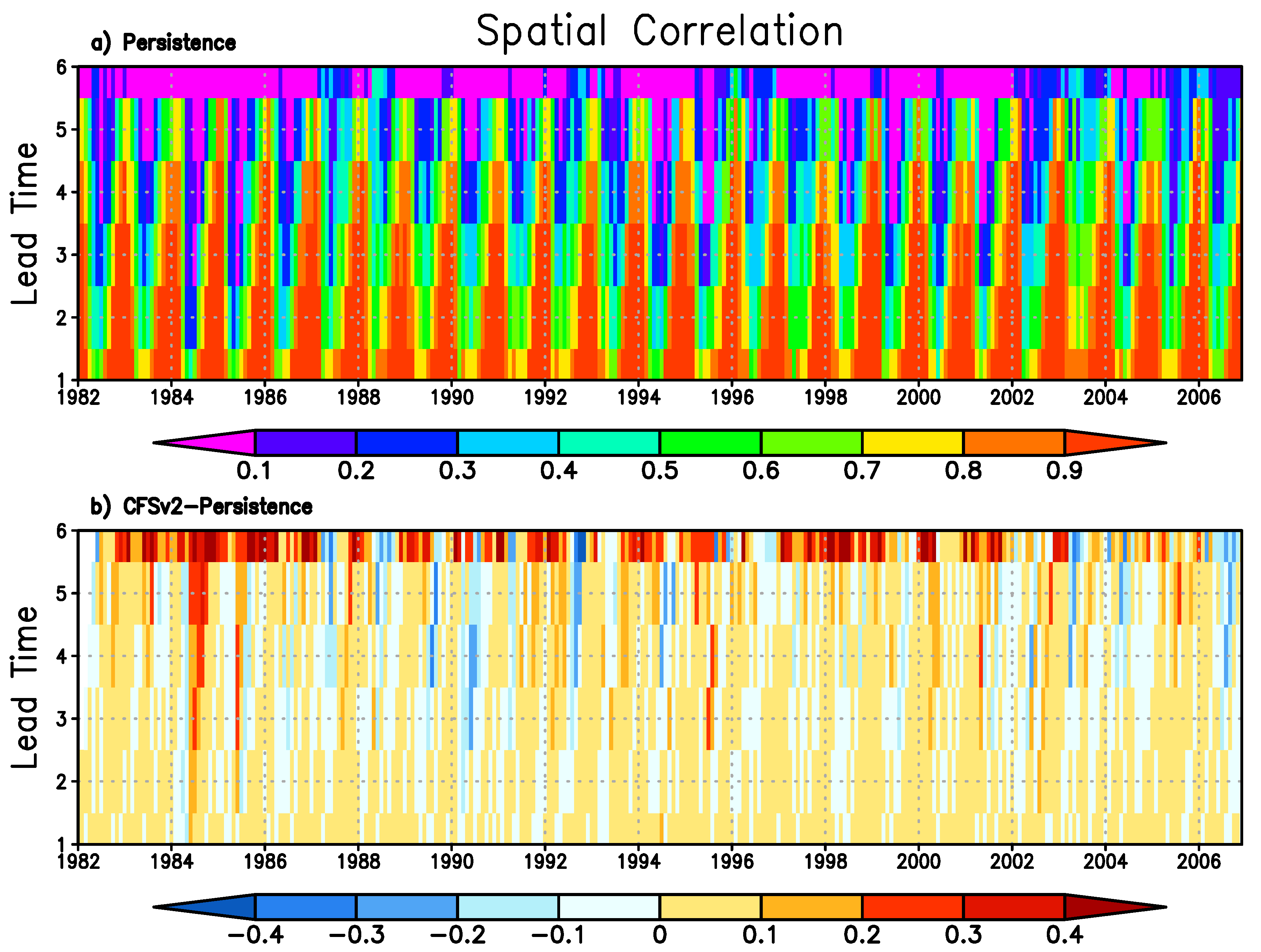
The spatial anomaly correlation is another metric that we used to evaluate the forecasts by measuring the spatial similarities between the forecast and observed SPI6 fields. Figure 4 shows the spatial anomaly correlation for each of the 300 forecasts at all six lead times from the persistence forecast and the difference between CFSv2 and the persistence forecast. It is evident that at shorter lead times, the spatial patterns of the SPI6 persistence forecast is very similar to the observed SPI6 fields with a spatial anomaly correlation between 0.6 and 0.9. As the lead time increases, such spatial similarities gradually disappear, and eventually at the six-month lead time, the correlation diminishes to near zero because the persistence forecast is the climatological mean. There is also a clear seasonal cycle for the spatial anomaly correlation. Relative to the persistence forecast, the CFSv2 forecast has a slightly large spatial correlation at the majority of the months and most of the lead times. This suggests that CFSv2 forecast in general provides spatially coherent forecast across the entire domain and it has positive contribution with respect to spatial patterns. The contribution is particularly larger at six-month lead time than other lead times.
Although the design of SPI has effectively removed the seasonality in precipitation, the persistence forecast skill and the contribution of the CFSv2 model to the drought forecast skill can still vary significantly with season and lead time. Figure 5 illustrates such variations with correlation coefficient and RMSE over two selected locations indicated in Figure 1a. These two locations are selected to represent two different climate zones. They are identified based on the watershed divisions and the Köppen–Geiger climate types (Peel et al. [30]) where China was divided into 17 large hydroclimatic regions (Lang et al. [18]). Location A is in the lower Yangtze River basin with a humid climate and annual precipitation about 1600 mm. Location B is in the semi-arid/arid northwest China with a dry climate and annual precipitation about 200 mm. During the cold-and-dry season (e.g., November to January), the persistence forecast can still be skillful at long lead times; however, during the warm-and-wet season (e.g., June to August), the skill drops quickly with lead time, especially at location B where rainfall during spring and summer experiences a stronger inter-annual variability than the prior season.
As shown in Figure 5, the contribution from the CFSv2 forecast to the drought forecast skill is mostly positive at all months and all lead times at these two locations. Negative contributions are seen in several month-lead combinations. The particular pattern of these combinations seem to suggest that the certain ensemble forecast runs from CFSv2 may have had abnormally poor performance. For example, at location B, June SPI6 forecast at the five-month lead time includes precipitation for February through June from forecast runs initialized between January 11 and February 10. These runs cause the CFSv2 forecast skill to be worse than that of the persistence forecast. The same forecast runs also contribute negatively to April SPI6 forecast at the three-month lead time. The cause of such poor model performance is beyond the scope of the study, nonetheless, identifying such problems could help model developers to conduct more focused diagnosis to improve the model.
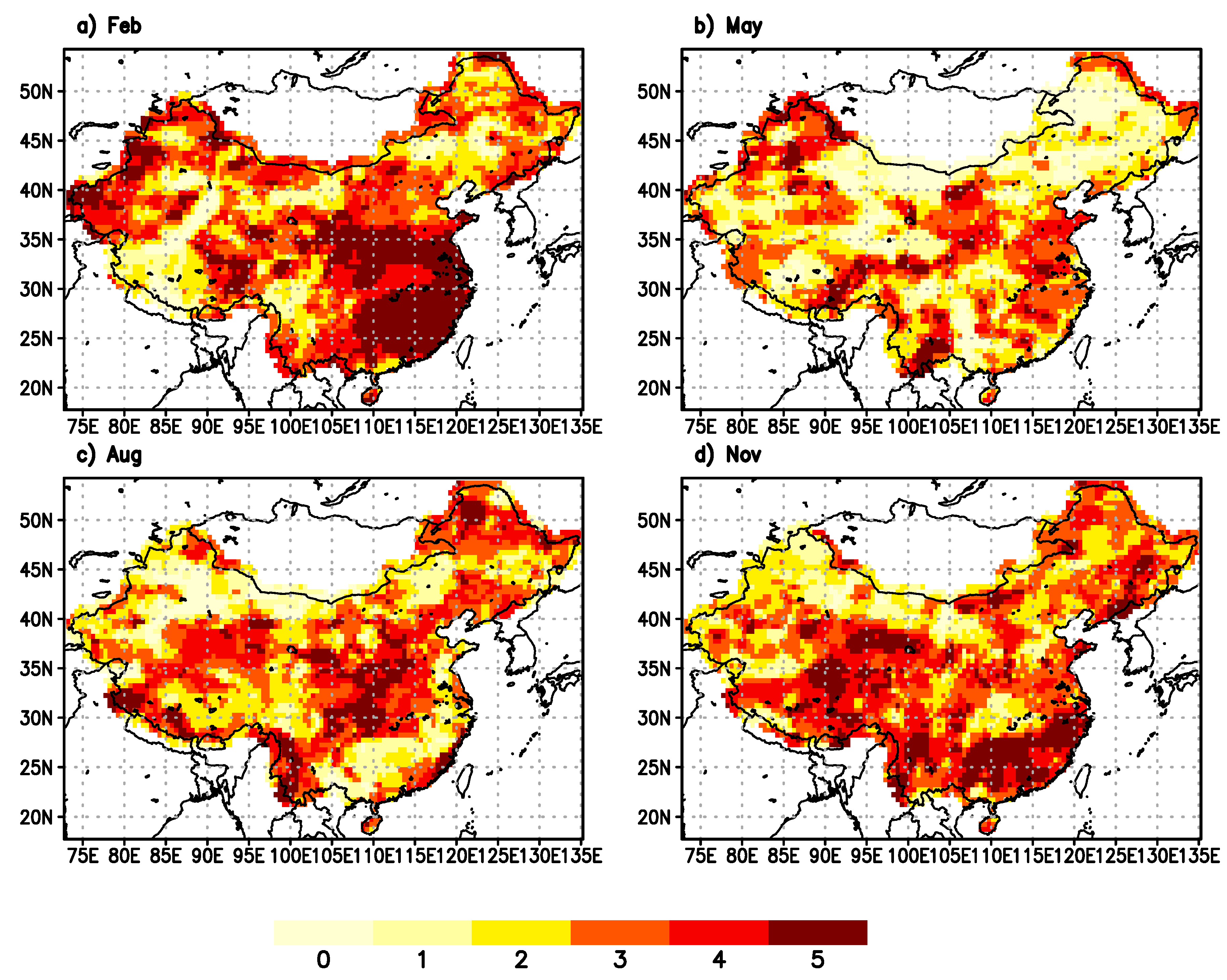
Based on the results in Figure 5, we can determine the maximum lead time when CFSv2 forecast always outperforms the persistence forecast for each month at a given location. This maximum lead time effectively represents the usefulness of CFSv2 forecast in improving seasonal drought prediction over persistence. The spatial distribution of the maximum lead time is presented in Figure 6 for February, May, August, and November SPI6 forecasts.
In February (target period: September to February), the CFSv2 forecast can add values to seasonal drought prediction for up to five months in a vast area in the east and southeast region, while the rest of the country also benefits from CFSv2 forecast for two to four months. Only a few spots in the northeast and Tibet region show no contributions from CFSv2 forecast. In May (target period: December to May), much larger areas in the north and northeast part of the country shows no contributions from CFSv2 forecast. Then, in August (target period: Mar to August), drought forecast over the central part of the country can benefit from CFSv2 forecast for up to five months, and finally in November (target period: June to November), this area shifts again to the southeast.
Figure 6 confirms that CFSv2 forecast in general helps to improve the drought forecast skill over the majority of the study region. Wherever the maximum lead time is above zero months, the CFSv2 forecast contributes positively to drought prediction skills. A similar result was obtained when measured by the RMSE. The figure also shows that the extent of contribution in lead time can vary strongly among different regions and different months. This suggests that the utilization of the CFSv2 forecast in other applications, such as seasonal hydrological predictions, needs to carefully consider these variations.
4. Discussion and Conclusions
There has been a gradual paradigm shift in weather agencies around the world to provide climate services related to drought and other climate extremes, which now relies heavily on forecasts at subseasonal–seasonal time scales from dynamic climate models. Thus, understanding the strength and weakness of these models is crucial for developing those applications and services. This paper presents an evaluation of the seasonal forecasts from the NCEP CFSv2 model over China with a focus on its ability to outperform the SPI6 persistence forecast that is solely based on historical observations.
We concatenated observed monthly precipitation with CFSv2 forecast in the following months to create CFSv2-based SPI6 forecast at various lead times. Taking 25-year (1982-2006) CFSv2 reforecast dataset and observed monthly precipitation analysis, we quantified the contribution of the CFSv2 model to improving drought forecast skills upon persistence forecast using the correlation coefficient, RMSE and their skill scores.
We find that the SPI6 persistence forecast and CFSv2 based forecast are, on average, skillful up to about four months of lead time. This is consistent with finding from several other studies (e.g., Lyon et al. [3], Yoon et al. [31], Quan et al. [4], Dutra et al. [26], and others). As lead time increases, the skill from the SPI6 persistence forecast and the CFSv2 forecast declines as expected. Despite the high skill from the persistence forecast at the short lead time, the CFSv2 still provides marginal improvements to forecast skills in most of the study domain. At longer lead times, the improvement brought by CFSv2 forecast becomes more pronounced, especially over the east and southeast part of China. Thus, the CFSv2 forecast provides more added value at longer lead times, even when the model forecast skill itself declines with lead time.
We need to recognize that both persistence forecast skill and the skill contributed by CFSv2 beyond the persistence have strong regionality and seasonality which is similar to what other studies have pointed out when using the CFS forecast ( Yoon et al. [31]), CFSv2 forecast ( Quan et al. [4]), and ECMWF seasonal forecast system ( Dutra et al. [26]; Dutra et al. [6]). The regional differences in forecast skill mainly exist between arid and humid regions. Skills are lower in arid regions during spring–summer and summer–autumn due to the stronger seasonal cycle of precipitation and the large inter-annual variability during these seasons. The regions where significant improvement was brought by the CFSv2 forecast are regions where the skill of the seasonal precipitation forecast are higher in China (Lang et al. [18]). In terms of seasonality, the seasonal cycle of precipitation and its inter-annual variability both play an important role in determining the persistence forecast skill. The persistence forecast skill is greatest during a region’s climatological dry season and is least during a wet season, the findings are consistent with Yoon et al. [31] and Quan et al. [4]. The skill beyond persistence contributed by CFSv2 also varies with season, and such variations seem to be affected occasionally by the poor model performance during certain initialization periods, as seen in Figure 5. The causes for such poor model performance requires further investigation.
There are situations where CFSv2 has no or sometimes even negative contribution, to drought forecast skill with respect to the persistence forecast. This leads to important questions related to enhancing precipitation forecast skill from dynamical climate models and how forecasts from dynamical climate models should be used to develop other applications and services. For example, seasonal hydrological prediction that uses seasonal temperature and precipitation forecast from dynamical models such as CFSv2 or NMME models should not only correct the bias in these forecast but also explicitly consider the skills of these forecast in various regions. Bias correction alone is not sufficient to make these forecast more skillful and useful. In regions where these climate models provide negative contributions to overall forecast skill, it is better to ignore the CFSv2 forecast and stay with the persistence forecast.
It is also worth mentioning that the current study treated the forecast as a deterministic forecast by using only the ensemble mean, which will lose some of the forecast information. An ensemble prediction approach can also be interpreted in a probabilistic way with the consideration of ensemble spread. A full evaluation of the ensemble prediction with probabilistic metrics will likely offer additional insights, and is granted for future studies.
To advance the seasonal drought forecast capability in China, obtaining high quality observations of precipitation, temperature, and soil moisture are still the most critical task. The proper use of the seasonal forecast from dynamical models including CFSv2 and NMME models provides a feasible route to improve skills and reliability. Such effort will nevertheless contribute to drought mitigation and water resource management in China.
Author Contributions
L.L. and Q.D. conceived and designed the experiment; Y.L. performed the experiments; Y.L. and L.L. analyzed the data; Z.L. and A.Y. contributed materials and analysis tools; Y.L. and L.L. wrote the paper. All authors have read and agreed to the published version of the manuscript.
Funding
This research was funded by Foundation for Excellent Young Scholars Training Program in Yunnan Province of Yunnan University (Grant No. 2018YDJQ017) and by the National Natural Science Foundation of China (Grant No. 41907147).
Acknowledgments
Monthly mean time series of CFSv2 precipitation were obtained from NOAA National Centers for Environmental Information (NCEI) at http://nomads.ncdc.noaa.gov/data.php?name=access#cfs-refor-data. Monthly mean time series of gauge-based analysis of daily precipitation over East Asia are obtained from NOAA National Centers for Environmental Prediction (NCEP) Climate Prediction Center (CPC) at ftp://ftp.cpc.ncep.noaa.gov/precip/xie/EAG/EA_V0409. We thank the three anonymous reviewers for their constructive comments.
Conflicts of Interest
The authors declare no conflict of interest.
References
- Ministry of Civil Affairs of the People’s Republic of China. China Civil Affairs’ Statistical Yearbook; China Statistics Press: Beijing, China, 2012.
- McKee, T.B.; Doesken, N.J.; Kleist, J. The relationship of drought frequency and duration to time scales. In Proceedings of the 8th Conference on Applied Climatology, Anaheim, CA, USA, 17–22 January 1993; American Meteorological Society: Boston, MA, USA; Volume 17, pp. 179–183. [Google Scholar]
- Lyon, B.; Bell, M.A.; Tippett, M.K.; Kumar, A.; Hoerling, M.P.; Quan, X.W.; Wang, H. Baseline probabilities for the seasonal prediction of meteorological drought. J. Appl. Meteorol. Climatol. 2012, 51, 1222–1237. [Google Scholar] [CrossRef]
- Quan, X.W.; Hoerling, M.P.; Lyon, B.; Kumar, A.; Bell, M.A.; Tippett, M.K.; Wang, H. Prospects for dynamical prediction of meteorological drought. J. Appl. Meteorol. Climatol. 2012, 51, 1238–1252. [Google Scholar] [CrossRef]
- Dutra, E.; Wetterhall, F.; Giuseppe, F.D.; Naumann, G.; Barbosa, P.; Vogt, J.; Pozzi, W.; Pappenberger, F. Global meteorological drought—Part 1: Probabilistic monitoring. Hydrol. Earth Syst. Sci. 2014, 18, 2657–2667. [Google Scholar] [CrossRef] [Green Version]
- Dutra, E.; Pozzi, W.; Wetterhall, F.; Giuseppe, F.D.; Magnusson, L.; Naumann, G.; Barbosa, P.; Vogt, J.; Pappenberger, F. Global meteorological drought—Part 2: Seasonal forecasts. Hydrol. Earth Syst. Sci. 2014, 18, 2669–2678. [Google Scholar] [CrossRef] [Green Version]
- Saha, S.; Moorthi, S.; Wu, X.; Wang, J.; Nadiga, P.; Tripp, P.; Behringer, D.; Hou, Y.; Chuang, H.; Iredell, M.; et al. The NCEP climate forecast system version 2. J. Clim. 2014, 27, 2185–2208. [Google Scholar] [CrossRef]
- Weisheimer, A.; Doblas-Reyes, F.J.; Palmer, T.N.; Alessandri, A.; Arribas, A.; Déqué, M.; Keenlyside, N.; MacVean, M.; Navarra, A.; Rogel, P. ENSEMBLES: A new multi-model ensemble for seasonal-to-annual predictions—Skill and progress beyond DEMETER in forecasting tropical Pacific SST. Geophys. Res. Lett. 2009, 36, L21711. [Google Scholar] [CrossRef] [Green Version]
- Kirtman, B.P.; Min, D.; Infanti, J.M.; Kinter, J.L., III; Paolino, D.A.; Zhang, Q.; van den Dool, H.; Saha, S.; Mendez, M.P.; Becker, E.; et al. The North American multimodel ensemble: Phase-1 seasonal-to-interannual prediction; phase-2 toward developing intraseasonal prediction. Bull. Am. Meteorol. Soc. 2014, 95, 585–601. [Google Scholar] [CrossRef]
- Luo, L.; Wood, E.F.; Pan, M. Bayesian merging of multiple climate model forecasts for seasonal hydrological predictions. J. Geophys. Res. 2007, 112, D10102. [Google Scholar] [CrossRef] [Green Version]
- Luo, L.; Wood, E.F. Use of Bayesian merging techniques in a multi-model seasonal hydrologic ensemble prediction system for the Eastern U.S. J. Hydrometeol. 2008, 5, 866–884. [Google Scholar] [CrossRef]
- Mo, K.C.; Lettenmaier, D.P. Hydrologic Prediction over the Conterminous United States Using the National Multi-Model Ensemble. J. Hydrometeorol. 2014, 15, 1457–1472. [Google Scholar] [CrossRef]
- Yuan, X.; Wood, E.F.; Luo, L.; Pan, M. A first look at Climate Forecast System version 2 (CFSv2) for hydrological seasonal prediction. Geophys. Res. Lett. 2011, 38, L13402. [Google Scholar] [CrossRef] [Green Version]
- Yuan, X.; Wood, E.F.; Roundy, J.K.; Pan, M. CFSv2-Based Seasonal Hydroclimatic Forecasts over the Conterminous United States. J. Clim. 2013, 26, 4828–4847. [Google Scholar] [CrossRef]
- Yuan, X.; Roundy, J.K.; Wood, E.F.; Sheffield, J. Seasonal Forecasting of Global Hydrologic Extremes: System Development and Evaluation over GEWEX Basins. Bull. Am. Meteorol. Soc. 2015, 96, 1895–1912. [Google Scholar] [CrossRef]
- Mo, K.C.; Lyon, B. Global Meteorological Drought Prediction Using the North American Multi-Model Ensemble. J. Hydrometeorol. 2015, 16, 1409–1424. [Google Scholar] [CrossRef]
- Kim, H.M.; Webster, P.J.; Curry, J.A. Seasonal prediction skill of ECMWF System 4 and NCEP CFSv2 retrospective forecast for the Northern Hemisphere Winter. Clim. Dyn. 2012, 39, 2957–2973. [Google Scholar] [CrossRef] [Green Version]
- Lang, Y.; Ye, A.; Gong, W.; Miao, C.; Di, Z.; Xu, J.; Liu, Y.; Luo, L.; Duan, Q. Evaluating skill of seasonal precipitation and temperature predictions of NCEP CFSv2 forecasts over 17 hydroclimatic regions in China. J. Hydrometeorol. 2014, 15, 1546–1559. [Google Scholar] [CrossRef]
- Luo, L.; Zhang, Y. Did we see the 2011 summer heat wave coming? Geophys. Res. Lett. 2012, 39, L09708. [Google Scholar] [CrossRef]
- Luo, L.; Tang, W.; Lin, Z.; Wood, E.F. Evaluation of summer temperature and precipitation predictions from NCEP CFSV2 retrospective forecast over China. Clim. Dyn. 2013, 41, 2213–2230. [Google Scholar] [CrossRef]
- Mo, K.C.; Shukla, S.; Lettenmaier, D.P.; Chen, L.C. Do Climate Forecast System (CFSv2) forecasts improve seasonal soil moisture prediction? Geophys. Res. Lett. 2012, 39. [Google Scholar] [CrossRef]
- Riddle, E.E.; Butler, A.H.; Furtado, J.C.; Cohen, J.L.; Kumar, A. CFSv2 ensemble prediction of the wintertime Arctic Oscillation. Clim. Dyn. 2013, 41, 1099–1116. [Google Scholar] [CrossRef]
- Saha, S.K.; Sujith, K.; Pokhrel, S.; Chaudhari, H.S.; Hazra, A. Predictability of Global Monsoon Rainfall in NCEP CFSv2. Clim. Dyn. 2015, 47, 1693–1715. [Google Scholar] [CrossRef]
- Xie, P.; Chen, M.; Yang, S.; Yatagai, A.; Hayasaka, T.; Fukushima, Y.; Liu, C. A Gauge-Based Analysis of Daily Precipitation over East Asia. J. Hydrometeorol. 2007, 8, 607–626. [Google Scholar] [CrossRef]
- Guttman, N.B. Accepting the standardized precipitation index: A calculation algorithm. J. Am. Water Resour. Assoc. 1999, 35, 311–322. [Google Scholar] [CrossRef]
- Dutra, E.; Giuseppe, F.D.; Wetterhall, F.; Pappenberger, F. Seasonal forecasts of droughts in African basins using the Standardized Precipitation Index. Hydrol. Earth Syst. Sci. 2013, 17, 2359–2373. [Google Scholar] [CrossRef] [Green Version]
- Wilks, D.S. Statistical Methods in the Atmospheric Sciences, Third Edition. Int. Geophys. Ser. 2011, 100, 676. [Google Scholar]
- Murphy, A.H.; Epstein, E.S. Skill Scores and Correlation Coefficients in Model Verification. Mon. Weather. Rev. 1989, 117, 572–582. [Google Scholar] [CrossRef] [Green Version]
- Krishnamurti, T.N.; Rajendran, K.; Vijaya Kumar, T.S.V.; Lord, S.; Toth, Z.; Zou, X.; Cocke, S.; Ahlquist, J.E.; Navon, I.M. Improved skill for the anomaly correlation of geopotential heights at 500 hPa. Mon. Weather. Rev. 2003, 131, 1082–1102. [Google Scholar] [CrossRef] [Green Version]
- Peel, M.C.; Finlayson, B.L.; McMahon, T.A. Updated world map of the Köppen-Geiger climate classification. Hydrol. Earth Syst. Sci. 2007, 11, 1633–1644. [Google Scholar] [CrossRef] [Green Version]
- Yoon, J.; Mo, K.; Wood, E.F. Dynamic-Model-Based Seasonal Prediction of Meteorological Drought over the Contiguous United States. J. Hydrometeorol. 2012, 13, 463–482. [Google Scholar] [CrossRef]
Figure 1.
Skill of the baseline persistence forecast measured by temporal correlation coefficient (left column) and root mean square error (RMSE) (right column) at the 1-month (top), 3-month (middle), and 5-month lead times. Locations A and B indicated in panel (a) were used in later analyses.
Figure 1.
Skill of the baseline persistence forecast measured by temporal correlation coefficient (left column) and root mean square error (RMSE) (right column) at the 1-month (top), 3-month (middle), and 5-month lead times. Locations A and B indicated in panel (a) were used in later analyses.

Figure 2.
Similar to Figure 1, but for the difference in skills between the Climate Forecast System version 2 (CFSv2) forecast and persistence forecast.
Figure 2.
Similar to Figure 1, but for the difference in skills between the Climate Forecast System version 2 (CFSv2) forecast and persistence forecast.

Figure 3.
Similar to Figure 1 but showing the skill scores of temporal anomaly correlation (TAC) and root mean square error (RMSE) for the CFSv2 forecast at three different lead times with the six-month standard precipitation index (SPI6) persistence forecast as the reference forecast.
Figure 3.
Similar to Figure 1 but showing the skill scores of temporal anomaly correlation (TAC) and root mean square error (RMSE) for the CFSv2 forecast at three different lead times with the six-month standard precipitation index (SPI6) persistence forecast as the reference forecast.

Figure 4.
The spatial anomaly correlations of all 300 forecasts (horizontal axis) with six lead times (vertical axis) from the persistence forecast (a) and the differences between the CFSv2 forecast and persistence forecast (b).
Figure 4.
The spatial anomaly correlations of all 300 forecasts (horizontal axis) with six lead times (vertical axis) from the persistence forecast (a) and the differences between the CFSv2 forecast and persistence forecast (b).

Figure 5.
Variation of forecast skill in the baseline SPI6 persistence forecast (rows 1 and 3) and the changes of forecast skill in the CFSv2 forecast (rows 2 and 4) in two selected locations marked in Figure 1a to represent two distinct climate zones. The forecast skill was measured by correlation coefficient in the top two rows (a–d) and by the RMSE in the bottom tow rows (e–h).

Figure 6.
The maximum lead time in months that the CFSv2 precipitation forecast shows better skills than persistence measured by correlation TAC. A similar result was obtained when measured by the RMSE.
Figure 6.
The maximum lead time in months that the CFSv2 precipitation forecast shows better skills than persistence measured by correlation TAC. A similar result was obtained when measured by the RMSE.

© 2020 by the authors. Licensee MDPI, Basel, Switzerland. This article is an open access article distributed under the terms and conditions of the Creative Commons Attribution (CC BY) license (http://creativecommons.org/licenses/by/4.0/).
Share and Cite
MDPI and ACS Style
Lang, Y.; Luo, L.; Ye, A.; Duan, Q. Do CFSv2 Seasonal Forecasts Help Improve the Forecast of Meteorological Drought over Mainland China? Water 2020, 12, 2010. https://0-doi-org.brum.beds.ac.uk/10.3390/w12072010
AMA Style
Lang Y, Luo L, Ye A, Duan Q. Do CFSv2 Seasonal Forecasts Help Improve the Forecast of Meteorological Drought over Mainland China? Water. 2020; 12(7):2010. https://0-doi-org.brum.beds.ac.uk/10.3390/w12072010
Chicago/Turabian StyleLang, Yang, Lifeng Luo, Aizhong Ye, and Qingyun Duan. 2020. "Do CFSv2 Seasonal Forecasts Help Improve the Forecast of Meteorological Drought over Mainland China?" Water 12, no. 7: 2010. https://0-doi-org.brum.beds.ac.uk/10.3390/w12072010
Note that from the first issue of 2016, this journal uses article numbers instead of page numbers. See further details here.