Evaluation of Design Storms and Critical Rainfall Durations for Flood Prediction in Partially Urbanized Catchments


1
University of Rijeka, Faculty of Civil Engineering, 51000 Rijeka, Croatia
2
University of Rijeka, Center for Artificial Intelligence and Cybersecurity, 51000 Rijeka, Croatia
*
Author to whom correspondence should be addressed.
Water 2020, 12(7), 2044; https://0-doi-org.brum.beds.ac.uk/10.3390/w12072044
Submission received: 19 June 2020
/
Revised: 14 July 2020
/
Accepted: 16 July 2020
/
Published: 18 July 2020
(This article belongs to the Special Issue Urban Rainwater and Flood Management)
Abstract
:This study investigates and compares several design storms for flood estimation in partially urbanized catchments. Six different design storms were considered: Euler II, alternating block method, average variability method, Huff’s curves, and uniform rainfall. Additionally, two extreme historical storms were included for comparison. A small, ungauged, partially urbanized catchment in Novigrad (Croatia) was chosen as a study area to account for the infiltration impact on the rainfall-runoff process. The performance of each design storm was assessed based on the flood modeling results, namely the water depth, water velocity, flow rate, and overall flood extent. Furthermore, several rainfall durations were considered to identify a critical scenario. The excess rainfall was computed using the Soil Conservation Service’s Curve Number method, and two-dimensional flooding simulations were performed by the HEC-RAS model. The results confirmed that the choice of the design storm and the rainfall duration has a significant impact on the flood modeling results. Overall, design storms constructed only from IDF curves overestimated flooding in comparison to historical events, whereas design storms derived from the analysis of observed temporal patterns matched or slightly underestimated the flooding results. Of the six considered design storms, the average variability method showed the closest agreement with historical storms.
1. Introduction
Prediction of flood hazards is a crucial part of flood risk assessment, flood risk management plans, and the design of flood protection measures. In the European Union (EU), a standardized procedure for flood mapping has been established by the EU Flood Directive (2007/60/EC) [1], which explicitly specifies which types of floods, flood parameters, and flood frequencies should be considered when assessing flood hazards. Due to a rising number of natural disasters, there is a growing interest in the EU regarding floods that occur directly from heavy rainfall, which are usually called pluvial floods [2]. Furthermore, because of a strongly interconnected rainfall-runoff process, as well as a rapid advancement of computational technology and the availability of high-resolution topographic data [3], pluvial floods are now simulated using integrated hydrological-hydraulic methods consisting of time-dependent 2D models and so-called rain-on-grid approaches [2,4,5,6,7]. However, a reliable flood prediction in small ungauged catchments remains difficult because of the lack of field observations needed to calibrate models [8,9,10,11].
There are two main approaches for flood assessment in ungauged catchments—the event based and the continuous-simulation method [12]. The event based methods simulate rainfall-runoff transformation of a design rainfall hyetograph of a given duration and return period [13], whereas the continuous-simulation methods are based on a similar transformation of a long (synthetic) rainfall time series and subsequent analysis of the flooding results to obtain a hydrograph of a corresponding return period [14]. The event based methods are more widely adopted and applied in engineering practice because of their simplicity, the availability of rainfall event data, and less computational time needed to perform the simulations. However, in event based approaches, one of the main sources of uncertainty is the hydrological data [10,12,14]. In particular, the rainfall input data, usually defined as a hyetograph—a temporal distribution of rainfall intensities—directly affects the runoff and corresponding water depths, water velocities, and flow rates [15,16]. Small catchments are particularly sensitive to the choice of the rainfall hyetograph because of the fast hydrological response of the catchment [8,9]. Therefore, one of the key elements in flood modeling is accurately representing the temporal distribution of rainfall intensities characteristic for a region. This is usually achieved by considering either a representative historical storm or by constructing a so-called design storm.
Design storms are synthetic hyetographs, which are widely used in engineering practice when designing stormwater drainage systems, assessing flood hazards, or proposing flood protection measures. A comprehensive overview of the evolution of the design storm concept was recently discussed by Watt and Marsalek [15]. Methods for generating design storms can be categorized into three main approaches [15,17]: (a) geometric pattern methods, which compute a single rainfall intensity from an Intensity-Duration-Frequency (IDF) curve and then redefine its temporal pattern by a simple geometric shape, (b) frequency based methods, which construct a hyetograph from the entire IDF curve, and (c) mass curves methods, which analyze temporal patterns of historical rainfall events to construct a dimensionless cumulative rainfall curve.
Geometric pattern methods are simple and easy to construct, but they do not necessarily reflect a temporal pattern of real storms at a given location and may produce biased runoff estimates [17]. In other words, this approach may be a good choice in some places, but not in others. Some popular methods belonging to this group include the triangular [18], double triangle [19], Sifalda [20] and linear-exponential method [21]. A recent overview and comparison of various geometric pattern methods is available in [22]. However, in this study, we focus primarily on the other two methods.
Frequency based methods use an entire set of intensities from IDF curves for all durations and a selected return period (or frequency). As such, these methods contain all maximum intensities in a single storm. Similar to the geometric pattern methods, they do not realistically represent the observed temporal patterns in a specific region [15,17]. The most popular frequency based methods are the Chicago design storm [23], the Alternating Block Method (ABM) [24], and the Euler method [25] (more commonly used in central Europe).
Mass curves methods, or so-called standardized profiles, are also widely used for stormwater drainage system design or flood hazard assessment. The main idea is that a dimensionless cumulative rainfall curve can be derived by analyzing historical rainfall patterns. In this way, the derived mass curves are unique and representative of a specific region. Some popular methods include the SCS design storms derived by the National Resources Conservation Services (NRCS) [26], where four types of curves are defined for the entire United States (U.S.), and Huff’s curves, which were also initially proposed for the U.S., but today, they are widely used in many other countries, such as China, Singapore, South Korea, Italy, and Slovenia [16,27,28,29]. Another design storm from this group is the Average Variability Method (AVM), developed by Pilgrim and Cordery [30,31], which has been used in Australia for many years now.
Selecting a suitable design storm is a matter of choice. Although some countries have regulations or recommendations regarding the best choice of the design storm, in other countries, there are no clear guidelines. Unfortunately, in some countries, such as Croatia, the design storm concept is overlooked, and a uniform hyetograph derived from IDF curves is still the preferred choice by the engineering community due to its simplicity. A recent EU project, Integrated Heavy Rain Risk Management (RAINMAN) [32,33], showed that all six central European countries that participated in the project (Austria, Croatia, Czech Republic, Germany, Hungary, and Poland) have different approaches to deriving a suitable design storm. Furthermore, the EU Flood Directive [1] does not provide any suggestion or recommendation on the choice of the design storm.
Considering that there is no consensus on which design storm is the most appropriate and there are numerous available methods to choose from, several recent studies attempted to assess, estimate, and compare different design storms in diverse regions and for various purposes. Al-Rawas et al. [34] assessed the characteristics of rainfall temporal distributions in arid mountainous and coastal regions and found that rainstorms are very similar in both regions, but that there is a significant difference between the observed rainfalls and standardized design storms. Nguyen et al. [35] also compared different design storm in the context of climate change and proposed an optimal storm pattern for southern Quebec region in Canada. Kimoto et al. [36] compared several design storms with observed storms in southern Arizona and concluded that observed storms were less intense than any considered design storms, especially for short durations. Pan et al. [28] similarly compared several different design storms for urban flooding in China, including an original modification to the Huff curve, which proved to be the most accurate. Pochwat et al. [37] evaluated different geometrical patterns of rainfall from the point of view of dimensioning retention facilities and reported that a rainfall pattern defined by a rising quadratic function produced the most critical values (largest retention volume). Na and Yoo [29] evaluated design storms in Korea by comparing them to historical rainfall events and reported that the ABM showed the best agreement with observed storms. Bezak et al. [16] assessed the impact of the rainfall duration and temporal rainfall distribution on the flood modeling in a rural catchment in Slovenia. They focused mostly on frequency based methods and Huff’s curves and concluded that the choice of the rainfall duration and design storm had a significant impact on the overall flooding results. Finally, Balbastre-Soldevila et al. [22] compared 11 well-known design storms for an urban drainage system application in Spain and recommended the AVM and a two-parameter Gamma function [38] as the most appropriate.
Another parameter related to design storms is the rainfall duration, which is defined as the duration that yields the maximum peak flow rates. In small and impervious catchments, the critical rainfall duration is usually related to the time of concentration [39]. However, for the design of retention basins/tanks or flood hazard assessment, the critical rainfall duration is related to both peak flow rate and maximum volume (or water depth) [35]. Furthermore, in more complex and partially urbanized catchments, the rainfall-runoff process is highly non-linear and depends on antecedent conditions, which further complicates the prediction of the critical rainfall duration [40].
Despite significant efforts in evaluating and deriving design storms, the engineering community is still far from a unified view on the optimal choice of a design storm for flood estimation. The lack of clear guidelines and recommendations can be explained by the fact that previous studies [13,16,22,28,29,34,35,36,37] had sometimes contradictory findings, which suggests that the choice of the optimal design storm depends on the catchment characteristics (size, slope, and land use [41]) and local climate (rainfall). Some of the studies that examined design storms were focused only on the hyetograph shape without an appropriate hydrological or hydraulic analysis [34,36]; some were focused only on stormwater drainage systems and urbanized catchments [22,28,37]; and some were based on a cross-comparison of different design storms without a suitable reference point (e.g., historical event) [16,22,37]. Furthermore, most of these studies agreed that their conclusions and recommendations should not be generalized and that more work is needed.
In view of these issues, the main aim of this study is to contribute to continuous progress in developing and understanding design storms. We extend previous studies by considering a partially urbanized catchment, where the rainfall-runoff process and infiltration have a more noticeable effect than in fully urbanized catchments. We focus on flood assessment and evaluate multiple flow parameters, such as the water depth, water velocity, flow rate, and flood extent, which provide a more comprehensive view of the impact of design storms. Furthermore, we compare the results to historical flood events to provide a more objective performance assessment of different design storms. Therefore, the specific aims of this study are: (a) to quantify the differences between several frequency based and mass curve methods when estimating multiple flood parameters required by the EU Flood Directive, (b) to quantify the differences between rainfall durations when estimating maximum flood parameters, and (c) to identify the optimal approach by validating different design storms against historical rainfall events.
2. Materials and Methods
2.1. Study Area
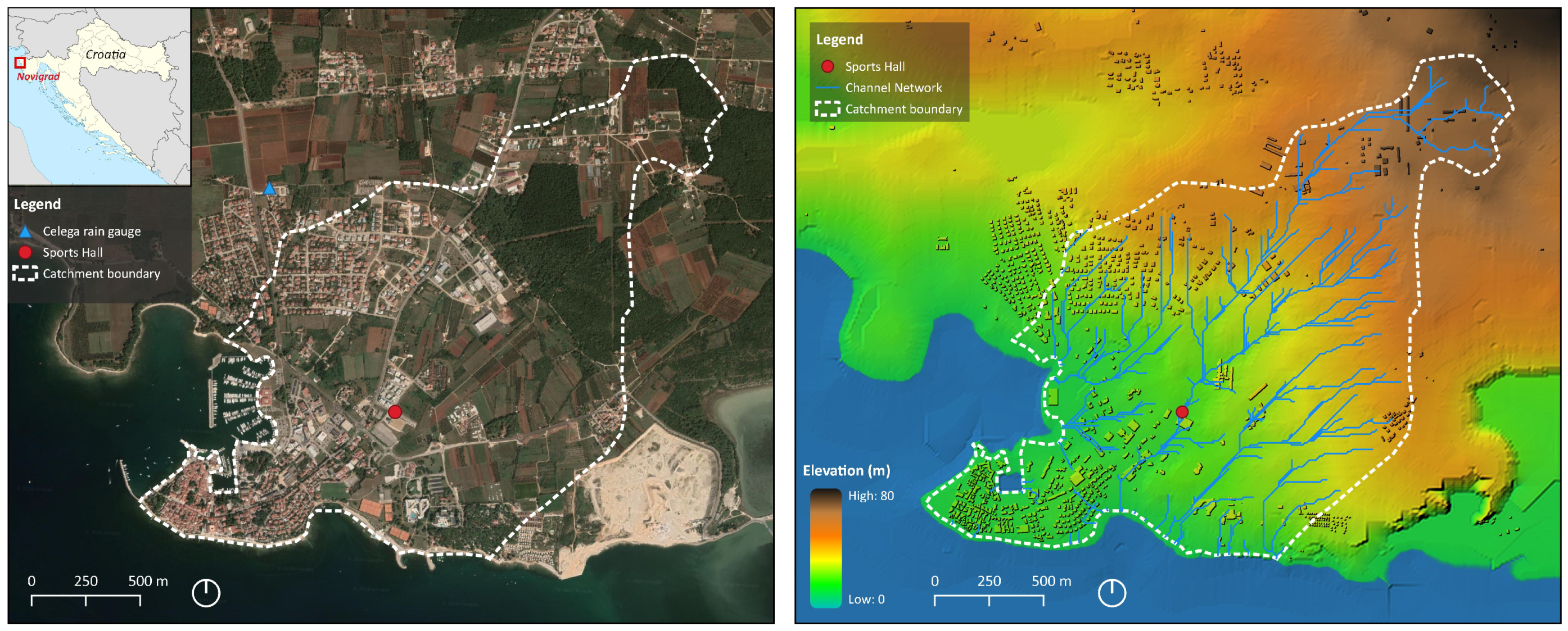
Novigrad is located in the northwestern part of Croatia, on the eastern coast of the Adriatic Sea (Figure 1). The primary reason for selecting it for a study area was the fact that this is a small partially urbanized catchment characterized by very intense short-term heavy rainfall observed at a local rain gauge and that this location has recently experienced extreme flooding. Additional criteria for selecting a suitable study area were: (a) the region should have above-average precipitation (short-term heavy rainfall) in relation to the national mean; (b) significant flooding should have been observed at the location, and the source of the flooding should have been primarily pluvial (without any fluvial influences); (c) long-term records from the rain gauge should be available; and (d) there should not be a well-developed stormwater drainage system in the catchment.
According to the last census from 2011, Novigrad has 4345 inhabitants. As a popular tourist destination, its population increases several times during the summer season. The city center, which dates back to medieval times, is located on a small peninsula. The area in its hinterland was traditionally used for agriculture, with orchards, olive groves, and vineyards. However, much of the agricultural lands have been partially urbanized over the years for recreational and tourism activities. Hotels and various other tourist facilities, including a yacht marina, are located along the coastline. Novigrad has a typical Mediterranean climate, with warm, dry summers and cool, mild winters. The main meteorological station Celega is located just outside the city center (see Figure 1). About 900 mm of precipitation fall on average annually, the majority of which refers to the autumn period. Short-term heavy rainfall episodes, however, regularly occur in the summer.
A Digital Elevation Model (DEM) for the Novigrad wider area was derived from a Croatia Base Map (HOK)—an official 1:5000 topographic map developed from aero-photogrammetry [42]. The elevation data were derived by vectorizing the contour lines from the HOK (with equidistance of 2.5–5 m). Following cartographic standards and recommendations [43,44], a corresponding DEM was derived with a m resolution by interpolating digitized contours using the GRASS module r.surf.contour, which generates surface raster map from elevation contours [45]. Elevations range from 0 to 80 m a.s.l. and gradually decrease towards the sea without any abrupt changes. A quasi Digital Surface Model (DSM) was created by combining DEM and a raster that included individual buildings, which were derived from the OpenStreetMap data and represented as surface elevation polygons. A Geographic Information System (GIS) analysis, namely the System for Automated Geoscientific Analyses (SAGA) [46], was used to delineate the catchment boundary and estimate the channel network (see Figure 1). SAGA uses a deterministic 8 method [46] to compute the flow direction, flow connectivity, channel network, and drainage catchments from a given DEM. A minimum Strahler order of 4 was set to determine the channel network, and the DEM was corrected by filling the sinks using the Wang and Liu method [47]. The algorithm produced over 20 subcatchments, but only those that gravitated towards the city center were selected and merged. The final catchment boundary was used to estimate the 2D flow area for the hydraulic model. Note that the channel network did not directly affect the hydraulic modeling and is illustrated here to better understand the catchment characteristics and anticipate the main flow paths. The overall catchment has an area of 3.08 km. Nearly half of this area (1.36 km) belongs to the subcatchment of the largest drainage system that flows east of the city center and where the most damaging consequences of floods have been documented.
This is a typical karst catchment composed of a limestone and dolomite bedrock covered by thick layers of terra rossa (a well-drained clay to silty-clay soil), where surface runoff very rarely occurs. Although the sanitary sewer covers the entire city, the stormwater drainage system is almost non-existent, except for several small road culverts and side ditches. Furthermore, no well-defined channels or gullies can be observed in the catchment.
2.2. Historical Storms and Floods in the Catchment
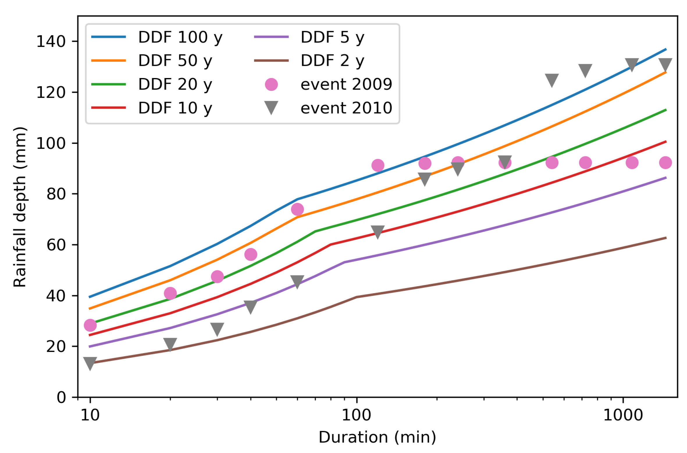
Two rainfall events observed at the Celega station in the period 2000–2012 were identified as extreme (they produced noticeable flooding in the Novigrad catchment) and thus were selected for a more detailed analysis and comparison to design storms. The first storm occurred on 21 July 2009 and lasted for 195 min with a total rainfall height of 92.3 mm and an average intensity of 28.4 mm h, which corresponds to a 50 y return period. Because of the temporal variability, maximum rainfall intensities for different durations correspond to return periods ranging from 20 to 100 years. Although no significant damage was reported, this short-term heavy storm resulted in high water levels in the Novigrad catchment.
The second event occurred on 19 September 2010 and lasted for 14 h with a total rainfall height of 130.7 mm and an average intensity of 9.8 mm h, which also corresponds to a 50 year return period. In this case, the event lasted longer than the one from 2009, with several peaks and intensities for different durations that corresponds to various return periods ranging from 2 to 100 years. In contrast to the 2009 event, this rainfall caused severe flooding, not only in Novigrad, but also over the entire northwestern part of Istria County, which declared a natural disaster. The greatest damage in Novigrad occurred in the newly-completed sports hall, which was completely flooded. Cars were trapped under the water, and most houses and buildings in the area were damaged by the flood and required assistance from civil protection. The GIS analysis revealed that the damaged sports hall was built in the middle of a hillslope hollow and at the center of the main flow path (see Figure 1).
Figure 2 shows a comparison of maximum rainfall depths for different durations observed during two historical events from 2009 and 2010 against rainfall Depth-Duration-Frequency (DDF) curves for the Celega station in Novigrad (1982–2012). From these two examples only, it becomes clear that assigning a single return period to a real storm is a delicate task that should be carried out with great care and consideration of all involved parameters, including the aim of the analysis and catchment characteristics. That being said, to compare design storms to historical rainfall events, we chose a 50 year return period as a representative parameter. This could be justified by the fact that both historical storms had a 50 year return period when their total rainfall depth and duration were considered.
2.3. Design Storms
In this study, we considered six different design storms. First was a uniform rainfall as a baseline scenario, which could be considered the simplest geometrical pattern method, having a rectangular shape. The uniform design storm was defined by a constant intensity computed from an IDF curve for a given rainfall duration and return period. This method is regularly used as a part of the Rational method for estimating peak flow rates and designing stormwater drainage systems [26]. In this study, however, we focus primarily on two other approaches that take into account at least some information about local rainfall variability.
Next, we chose two frequency based methods. The first one was the Euler II method [25], which is recommended by the German Association for Water, Wastewater and Waste (DWA-A 118E) and widely adopted in Germany and Austria for stormwater drainage design, as well as flood hazard assessments in urban areas. Note that the civil engineering community in Croatia traditionally adopts German guidelines and norms. However, it should also be noted that Croatia still does not have any regulative acts nor guidelines regarding the choice of a suitable design storm. The second approach was the Alternating Block Method (ABM) [24], which is widely known and applied in practice internationally.
For both considered frequency based methods, a total rainfall duration T was selected first, as well as a time interval ( min was chosen in this study to match the minimum value for which IDF curves are valid). Then, for each duration , the rainfall intensity was computed from an IDF curve (for a given return period). Next, the rainfall depth was computed for each duration, and incremental rainfall depth was found for each time interval by calculating differences between . The final step was to compute incremental intensities and reorder them according to a predefined pattern. For the Euler II method, were arranged in descending order, but the first third was flipped so that the highest intensity was located at one-third of the rainfall duration, Whereas the highest intensity for the ABM was placed at the center, and remaining were arranged in descending order alternately on each side of a hyetograph, starting on the right.
Finally, we focus on two mass curve methods, namely Huff’s curves [48,49] and the Average Variability Method (AVM) [30]. Huff’s curves were derived from selected historical precipitation records. Individual cumulative storms, or mass curves, were first transformed into a dimensionless form—a (0, 1) by (0, 1) space—by dividing the rainfall depth by the total rainfall and time by the total rainfall duration. Next, mass curves were categorized into four quartiles according to the time of the peak intensity (e.g., if the peak intensity occurred in the first quarter , the storm belonged to the first quartile; if it appeared in the second quarter , it belonged to a second quartile, etc.). A set of curves for each quartile was then intersected by vertical lines for every dimensionless duration from 0 to 1. Along each vertical line, a corresponding probability was determined, which was derived from the distribution of these intersections. Finally, the assigned probability points along each vertical line were connected with so-called isopleths. These isopleths comprise a set of Huff’s curves, and they usually range from 10% to 90% in increments of 10%. For example, a 50% curve represents a cumulative rainfall pattern, which is expected to be exceeded by half of all storms. For a more illustrative description of Huff’s curves, we recommend the work by Bonta et al. [49]. Note that nine isopleths combined with four quartiles produces 36 Huff’s curves, which is a large number of storms to analyze in practice. Furthermore, although some studies suggest that quartiles can be related to rainfall durations [50], we found no such evidence for storms in Istria County [32] nor for the neighboring coastal city Rijeka [51]. Therefore, in this study, we considered only the 50% (median) curve, which is usually recommended for engineering purposes [49,50]. We chose the 2nd quartile (Huff Q2) as a representative of the majority of historical storms, and we also included the 3rd quartile (Huff Q3) because it produced the most similar hyetograph to two considered historical storms.
The average variability method was similarly based on the analysis of selected historical precipitation records. Individual storms were first grouped by duration in several classes. Here, we chose the following four classes: (a) min, (b) min, (c) min, and (d) min. Next, each storm was divided into predefined intervals, which usually correspond to the resolution of the rainfall record (in this case, min). Each rainfall interval was ranked according to the rainfall depth in that interval. Once the intervals were ranked for all selected events, an average rank was assigned to every interval. Average rainfall depth was then computed for each rank, and a design storm pattern was obtained by arranging the intervals according to their rank. A more detailed description of the AVM with examples is available in [30,31]. In this study, a slight modification of AVM was applied, where the storms in each class were first transformed into a dimensionless form, just as for the Huff method. In both the Huff and average variability methods, the final hyetograph was constructed by assigning a rainfall depth and duration to a dimensionless mass curve and then computing the rainfall intensities for each interval.
For constructing all six design storm hyetographs, we used the IDF curves for the Celega station (1982–2012), which were recently updated as a part of the EU project RAINMAN [33]. Analysis of the rainfall patterns, required for the Huff and AVM method, were based on historical records with a 5 min resolution from the Celega station (2000–2012), as well as two additional stations in Istria County—Pula (1957–2017) and Pazin (1963–2017)—which are located 55 km south and 30 km southeast of Novigrad, respectively.
2.4. Excess Rainfall
Once all design storms had been constructed for each duration and selected return period, corresponding excess rainfall hyetographs were computed using the Soil Conservation Service’s (SCS) Curve Number (CN) method [26,52]. The SCS CN method was applied to convert the total to excess rainfall by estimating the initial and continuous losses. First, cumulative rainfall was computed from each hyetograph, and at each time interval, the following equation was applied:
where Q is the cumulative excess rainfall, P is the cumulative rainfall depth, is the initial abstraction, and S is the potential maximum retention after runoff begins, which is determined from the curve number CN. If millimeters are used as units for rainfall depth, S is:
The CN was determined from the land use and hydrological soil group. In the Novigrad catchment, the CN were determined considering the current land use and hydrological soil group B, which resulted in the following (averaged) distribution: weighted average CN = 70 for the pervious area covering 85% of the catchment and CN = 98 for the impervious area covering 15% of the catchment (more details on the distribution of individual cover types and their sizes are shown in Table 1).
Instead of calculating a composite CN number for the catchment, we computed the excess rainfall for each CN and then performed a weighted average of those values to obtain the excess rainfall for the entire catchment. This is a preferred approach for partially urbanized catchments, because the composite CN may underestimate peak runoff [52]. Finally, once the cumulative excess rainfall had been determined, the excess hyetograph was constructed as an input into the hydraulic flood model. Note that because of small size, the Celega station and the corresponding rainfall data could be considered uniform over the entire Novigrad catchment area.
2.5. Hydraulic Model
Flood simulations were performed by a Hydrologic Engineering Center-River Analysis System (HEC-RAS 5.0.7) using an unsteady 2D flow model [53]. HEC-RAS provides two sets of equations to solve the shallow water flow in two dimensions (2D), the Saint Venant (SV) equations (or full momentum) and Diffusion Wave (DW) equations, which were used in this study. In comparison to Saint Venant, DW equations are more efficient and less prone to accuracy loss when simulating rainfall-runoff processes [54]. HEC-RAS 2D and DW equations have been successfully applied in many other flood assessment studies under various conditions, different flood sources, and a wide range of catchment sizes [7,55,56].
A classical differential form of the diffusion wave equation is [53]:
where H is surface elevation, t is time, is the surface elevation gradient, q is source/sink flux term, and coefficient is [53]:
with hydraulic radius R and Manning’s roughness coefficient n. Once Equation (3) is solved, velocities can be found by computing [53]:
The DW equations were solved in HEC-RAS using a hybrid discretization scheme that combined finite differences and finite volumes to take advantage of orthogonality in grids. The finite differences scheme is used over orthogonal grids, whereas the finite volume method is used to discretize equations when the grid is not locally orthogonal and to approximate source terms, such as eddy viscosity [53]. An implicit solution scheme and variable time step were used for all simulations. To ensure the stability of the model, the time step was estimated according to the Courant–Friedrichs–Lewy (CFL) condition. For 2D DW equations, the recommendations state [53]:
where c is the flood wave celerity, is the time step, and is the cell size. Since the scheme is implicit, CFL can be larger than 1.0. In this study, we used a fully implicit scheme and set a maximum CFL to 2.0.
HEC-RAS 2D uses a sub-grid bathymetry approach [53], which means that each grid cell contains additional information on the hydraulic radius, volume, and cross-sectional area as a function of water depth. These characteristics were computed from bathymetry (DEM) in the pre-processing stage. Note that this approach allowed very fine bathymetry characteristics to be captured while using much larger computational grids in the hydraulic computation.
The geometry (spatial domain) was imported from a GIS analysis based on a DSM (DEM + buildings) with a 2 m resolution. An average m grid size was chosen to represent the entire domain, with internal (geometrical) boundaries of a higher resolution ( m) around the sports hall to ensure more accurate results at the location. A generated 2D mesh consisted of 38,499 cells, with an average face length of 10 m, average cell size of 100 m, maximum cell size 181 m, and minimum 22 m. Bottom friction in the DW approach was simulated by Manning’s equation. Therefore, a spatially varied Manning’s coefficient was set with values ranging from m s for roads to m s for agricultural lands.
Three boundary conditions were defined for flood simulations. First, an external boundary condition line was set along the catchment land boundary, with a total length of 5691 m. Next, an external boundary condition line was set along the catchment sea boundary (coastal line), with a total length of 3107 m. A normal depth condition with slope 0.01 was set along the land boundary line, whereas a stage hydrograph was set to a constant value of 0.0 m along the sea boundary line. Finally, a so-called rain-on-grid was set over the entire 2D computational area; in other words, a predefined hyetograph (excess rainfall computed by the SCS method) was uniformly distributed over each grid cell. The total simulation time for each scenario lasted for 6 h.
3. Results
3.1. Excess Rainfall
This section presents several results to illustrate the excess rainfall in comparison to total rainfall hyetographs for historical events and design storms.
3.1.1. Historical Events
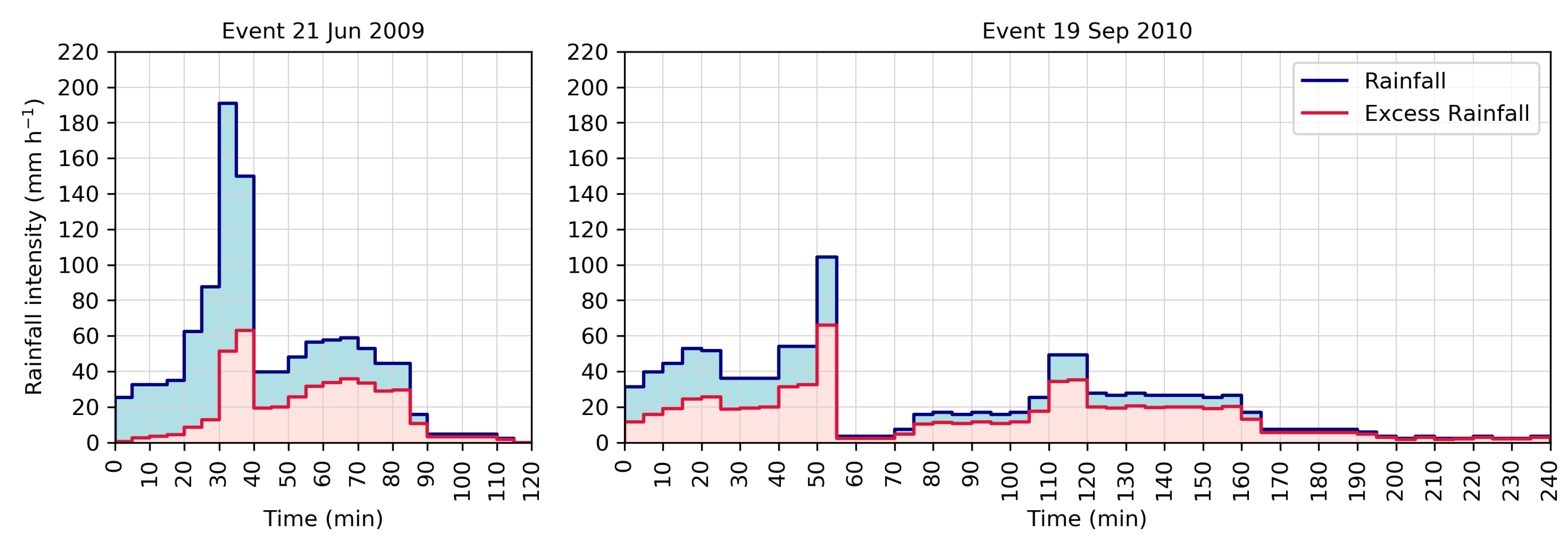
Figure 3 shows a rain intensity hyetograph for both historical storms, with total observed rainfall and excess rainfall computed by the SCS method for the Novigrad catchment. Although the duration of both considered events was longer, here we show only the main part of the storm. For the 2009 event, ninety-eight percent of total rainfall occurred during 2 h with an average intensity of 45.6 mm h, and for the 2010 event, seventy percent of total rainfall occurred during 4 h, with an average intensity of 22.4 mm h. The maximum 5 min intensity was 190.8 mm h for the shorter 2009 event and 104.4 mm h for the longer 2010 event. The maximum intensity for the excess rainfall, on the other hand, was almost identical in both cases, amounting to 63 mm h for the former and 66 mm h for the latter. This could be explained by the use of SCS method and the impact of initial abstraction and continuous infiltration. The maximum intensity for the 2010 event was less affected by the infiltration in comparison to the 2009 event because the maximum intensity in 2010 was preceded by a longer period of low-intensity rain.
3.1.2. Design Storms
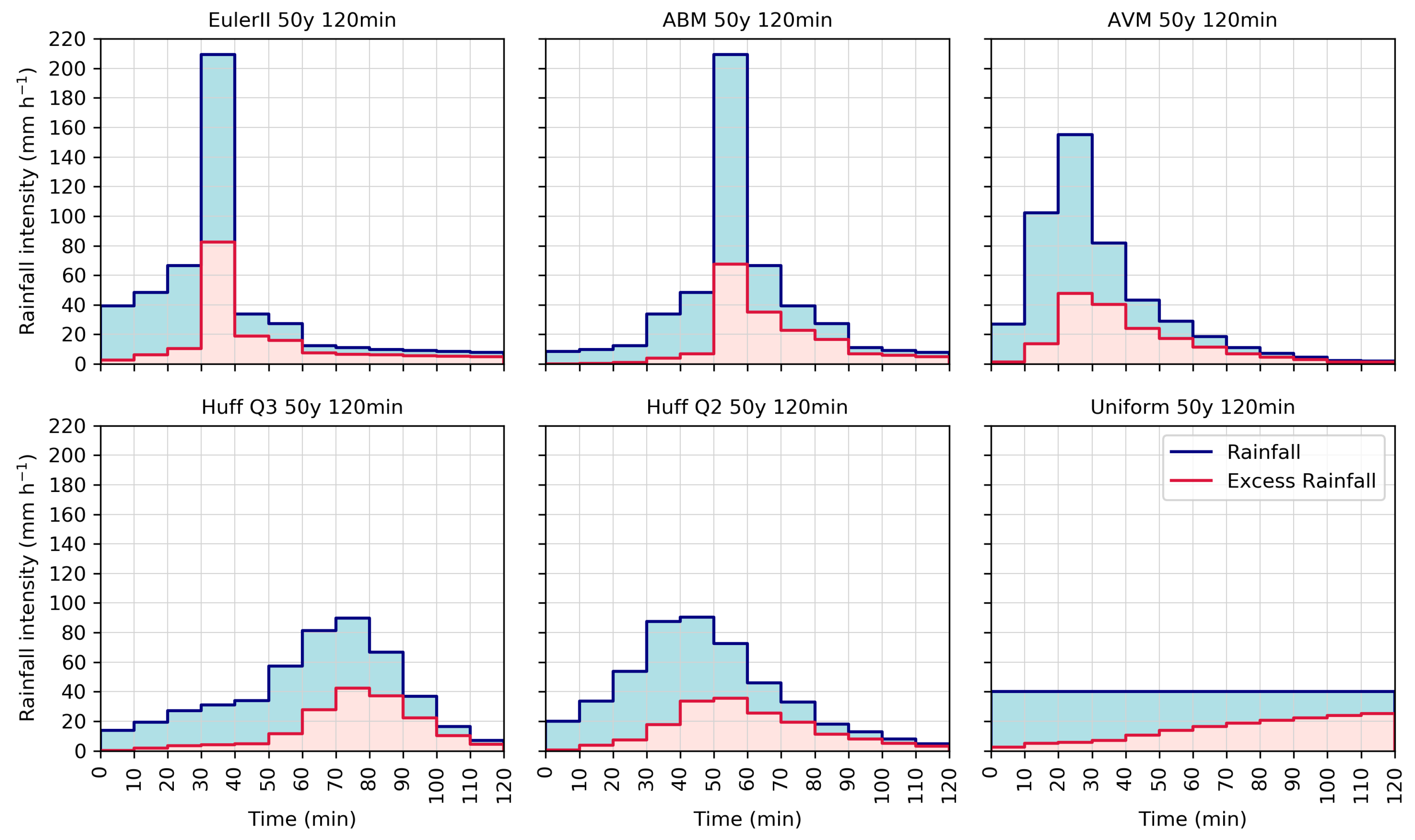
Design storms were generated using six different design storm approaches for a 50 year return period and a total duration of 2, 3, 4, and 6 h. Figure 4 shows the total and excess rain hyetograph for a 50 year return period, a 120 min duration, and a 10 min time interval. All considered design storms had the same average 2 h total rain intensity of 40.3 mm h computed from the IDF curve and excess rain intensity of 14.3 mm h.
Euler II and ABM had the highest 10 min intensity and the most pronounced temporal variability with a 5.2 peak-to-average intensity ratio. This was expected since they included maximum intensities for all durations up to 120 min. These two design storms were composed of identical 10 min block intensities, the main difference being that the peak intensity for Euler II was located at one-third of the total duration and for ABM at one half of the total duration. Because of these differences in the ordering of 10 min blocks and the use of the SCS method, the maximum 10 min excess rain intensity was slightly higher for the Euler II in comparison to the ABM design storm. Note that 10 min total and excess rain intensities for these two design storms exceeded the 5 min maximum intensity observed in both historical storms.
The design storm derived by the AVM had a lower maximum 10 min intensity in comparison to the Euler II and ABM design storms, but still showed a pronounced temporal variability with a 3.8 peak-to-average intensity ratio. The maximum 10 min total rain intensity fit between the 2009 and 2010 storms, whereas the excess rain intensity was just below the 2010 storm. The temporal pattern of AVM design storms reflected the fact that most observed storms at the Celega station had a peak in the first quarter of the rain duration.
Huff Q2 and Q3 design storms showed a similar 2.2 peak-to-average intensity ratio, which was lower than the AVM. The maximum 10 min total and excess rain intensity were lower than in both historical storms. The main difference between Huff Q2 and Q3 was the position of the peak intensity. This had some effect on the maximum excess rain intensity, which was slightly higher in the Huff Q3 design storm.
Finally, the uniform design storm was derived directly from the IDF curves for a 120 min duration. The peak intensity was equal to the average intensity and several times lower than in other design and historical storms. That being said, the peak excess rain intensity occurred near the end of the rain duration and was not significantly lower than the Huff Q2 design curve.
The design storms for other (longer) considered durations showed a similar pattern as the one described here. The duration of the storm did not change the qualitative conclusions on the relationship between these six approaches.
3.2. Flood Analysis
Flood analysis for the city of Novigrad was carried out in the HEC-RAS model for two historical events (21 June 2009 and 19 September 2010), as well as for six different design storms (Euler II, ABM, AVM, Huff Q2, Huff Q3, and uniform rainfall) in combination with four different durations (2, 3, 4, and 6 h). In total, 26 simulations were performed and processed.
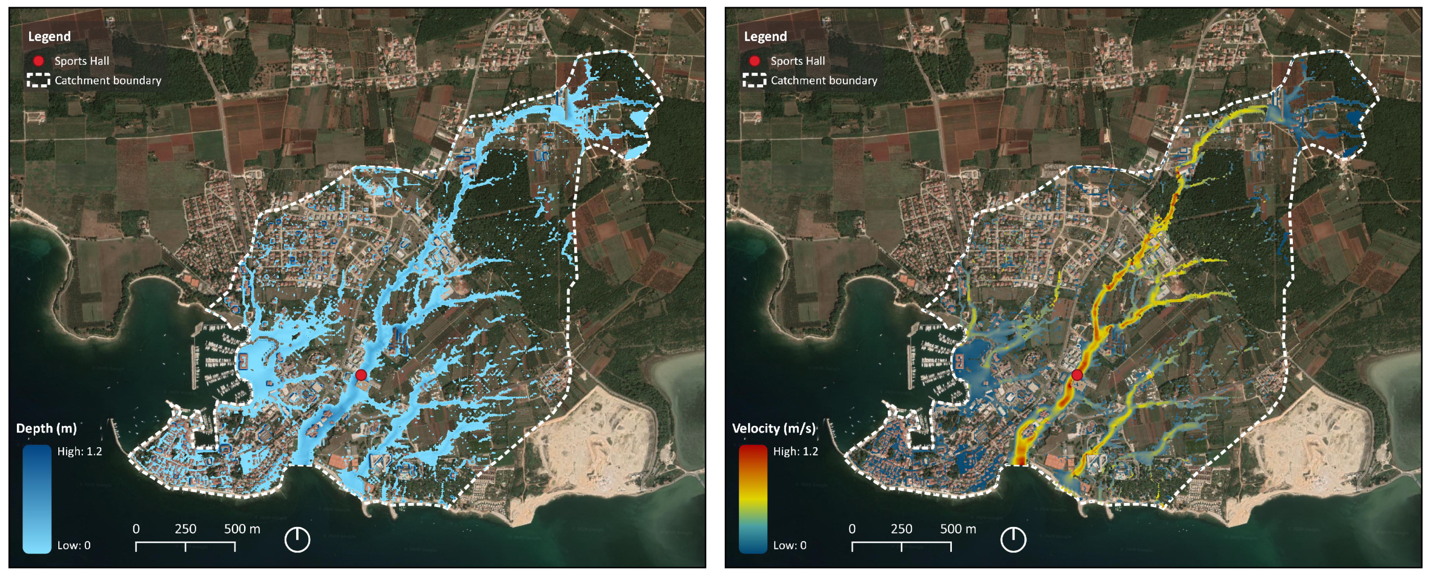
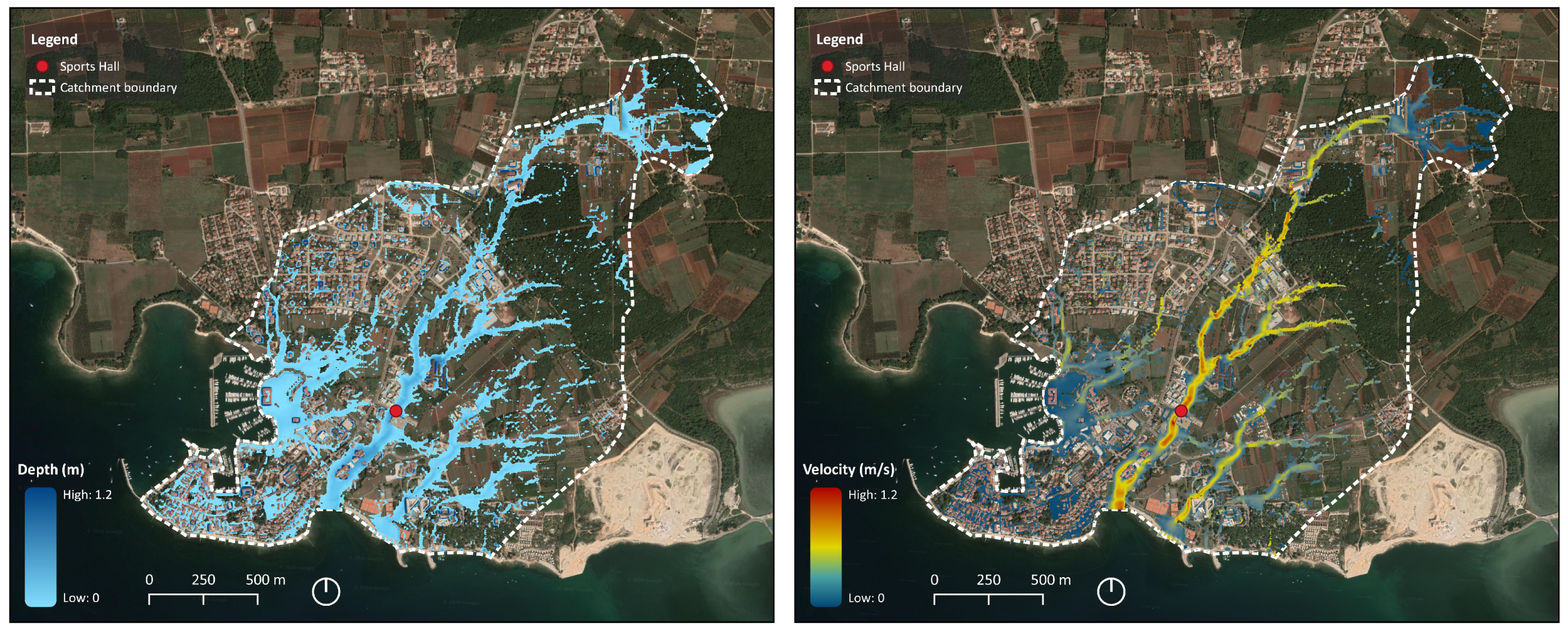
Figure 5 and Figure 6 show the flood modeling results—the spatial distribution of maximum water depths and velocities for the 2009 and 2010 storms in the Novigrad catchment, respectively. Several different flow phases were observed in the catchment; in the central and southeastern part of the catchment, sheet flow quickly transitioned to shallow concentrated flow through hillslope hollows and then entered the Adriatic Sea. In the more urbanized southwestern part of the catchment, the sheet flow was predominant with some shallow concentrated flows through streets and swales.
The overall flood extent, as well as the depth and velocity distribution were quite similar for both considered storm events. In comparison to 2010, the 2009 event showed slightly larger depths and higher velocities, although these differences were minor at the catchment scale. Water depths ranged from 0.1 to 1.2 m, and water velocities ranged from 0 to 1.2 m s. The largest depths and velocities were found along the main flow direction through a 100–200 m wide hollow in the central part of the catchment. As mentioned earlier, the sports hall that was flooded in 2010 was located just in the middle of this topographical depression and exposed to the largest water depths and velocities. Flood extent results for design storms showed a very similar pattern as the two historical storms; the differences were hardly distinguishable at the catchment scale; therefore, they are not shown here, and instead, only the maximum values are reported and discussed.
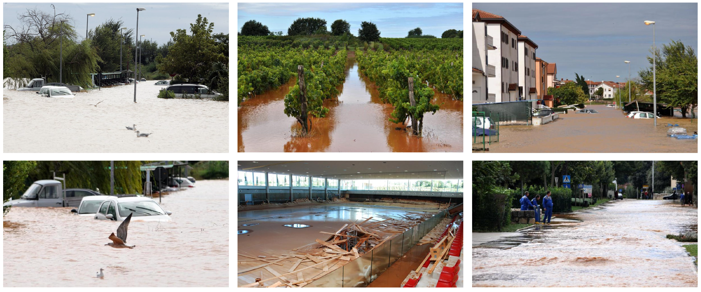
The validation of such extreme, but short-term, flood events is almost impossible in small ungauged basins. However, some reports and photos from field reporters and citizens are available in local newspapers. Therefore, in Figure 7, we show several photos of Novigrad and neighboring Umag area from 19–20 September 2010 for a qualitative comparison to the numerical results. The photos clearly show flooded streets and vineyards, vehicles under water, and the damaged sports hall in Novigrad.
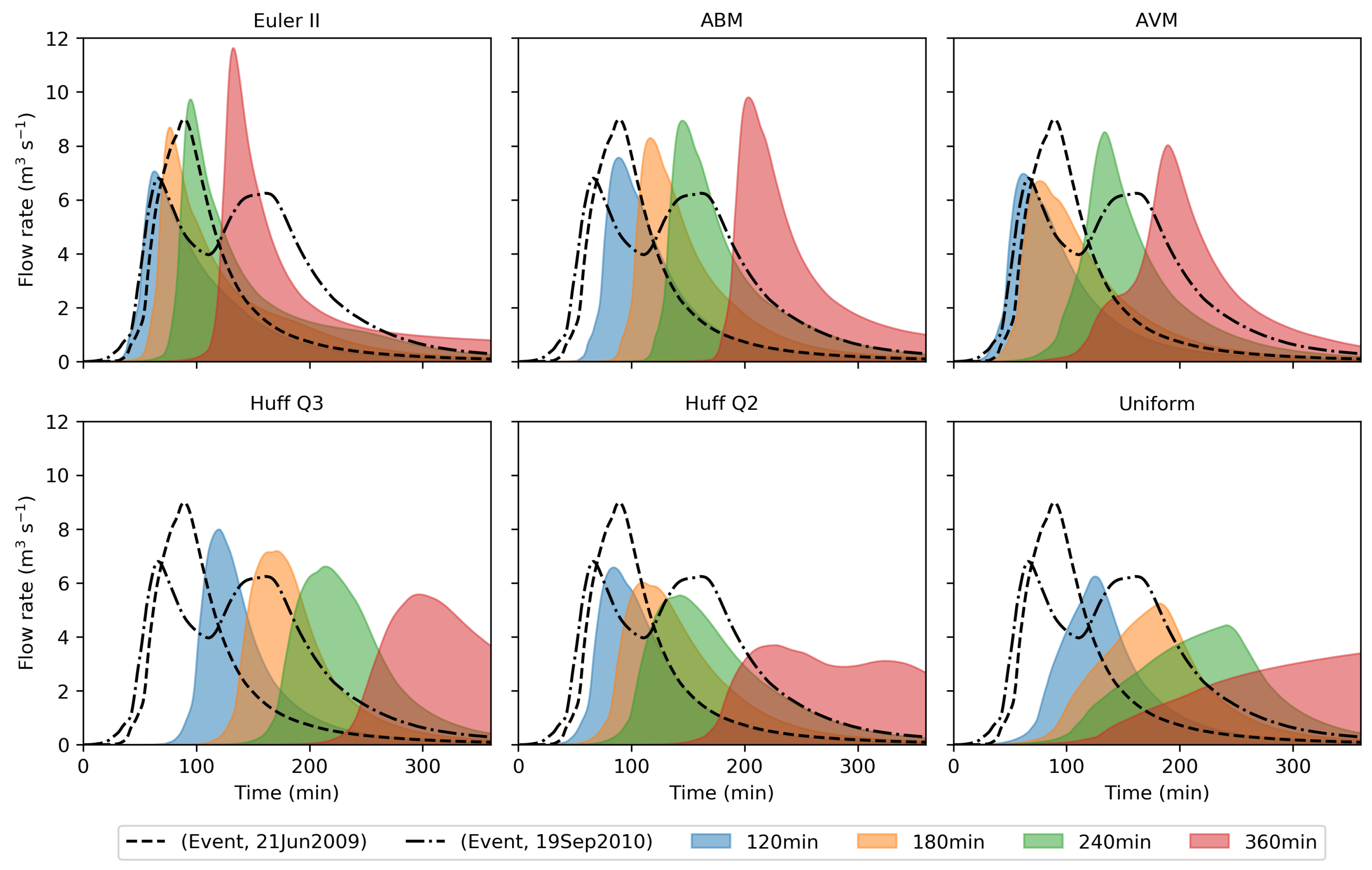
Figure 8 shows computed runoff hydrographs through the hillslope hollow just upstream from the sports hall (red dot in Figure 5 and Figure 6). The figure shows six panels; in each panel, the flow rates generated by the two historical events are compared to flow rates generated by one of the six considered design storms derived for different rainfall durations.
The 2009 event generated a single peak runoff hydrograph with a maximum flow rate of 8.98 m s and time to peak of 89 min. On the other hand, the 2010 event generated a double peak hydrograph, with maximum flow rates of 6.8 m s and 6.25 m s.
The peak flow rates generated by the Euler II design storm increased with longer storm durations, and the maximum values were found for the 6 h duration. The ABM storm similarly showed an increase of the peak flow rate with longer storm durations, where maximum values were also found for the 6 h duration. The AVM had very similar hydrographs for storm durations of 2 and 3 h, whereas the maximum values were found for the 4 h duration. Both Huff design storms generated hydrographs with a peak flow rate that decreased with a longer storm duration, and the maximum values were found for Huff Q3 design storm and a 2 h duration. Finally, the uniform design storm also showed a decrease in the peak flow rate with longer durations and had a maximum value for the 2 h duration. This shows that some design storms may produce higher flow rates for durations that exceed the time of concentration.
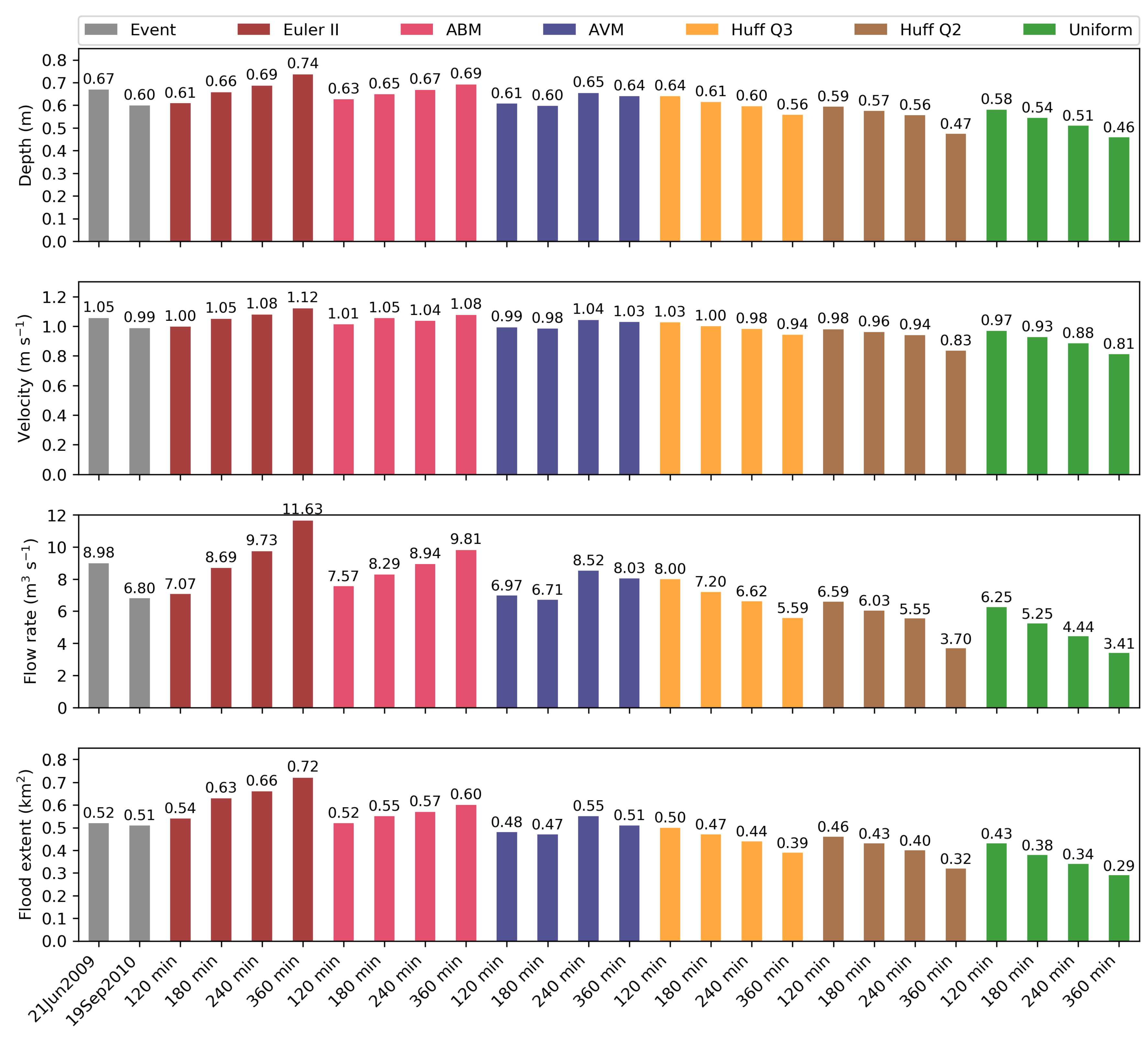
A more detailed comparison of flood results generated by different design storms and historical rainfall events is shown in Figure 9. In addition to peak flow rate, here we also compare the maximum water depth and velocity at the same location upstream from the sports hall, as well as the overall flood extent in the Novigrad catchment. The flood extent is defined as the total area where the maximum water depth exceeds 10 cm.
The 2009 event had a maximum water depth of 0.67 m and velocity of 1.05 m s, whereas the 2010 event had a slightly smaller flood impact with a maximum water depth of 0.6 m and velocity of 0.99 m s. In comparison, the Euler II design storm generated equal or higher water depths and velocities (depths ranging from 0.61 m to 0.74 m and velocities ranging from 1.0 to 1.12 m s). ABM design storm, similarly, generated equal or higher water depths and velocities (depths ranging from 0.63 to 0.69 m and velocities ranging from 1.01 to 1.08 m s). Both these design storms had maximum values for the longest duration (6 h), which exceeded the (more extreme) 2009 event. The AVM design storm generated similar water depths and velocities as two historical events (depths ranging from 0.6 m to 0.65 m and velocities ranging from 0.98 to 1.04 m s). Minimal values were almost identical to the 2010 events, while maximum values were very close to the 2009 event. Huff Q3 design storm also predicted water depths and velocities similar to two historical events (depths ranging from 0.56 m to 0.64 m and velocities ranging from 0.94 to 1.03 m s). However, maximal values were lower than the 2009 event, and minimal values were lower than the 2010 event. The Huff Q2 design storm predicted water depths and velocities slightly lower than two historical events (depths ranging from 0.47 m to 0.59 m and velocities ranging from 0.83 to 0.98 m s). As expected, the uniform design storm predicted the lowest water depths and velocities (depths ranging from 0.46 m to 0.58 m and velocities ranging from 0.81 to 0.97 m s). Overall, the differences in water depth and velocity between the historical events and design storms were not substantial and were inside a ±30% error margin. Maximum values by the ABM, AVM, and Huff Q3 design storm agreed well with the two historical storms.
In contrast to water depths and velocities, differences in peak flow rates were more noticeable. For the 2009 and 2010 events, peak flow rates were 8.98 and 6.80 m s, respectively. The Euler II peak flow rates exceeded these values and ranged from 7.07 to 11.63 m s. The ABM peak flow rates also exceeded two historical events and ranged from 7.57 to 9.81 m s. The peak flow rates for the AVM design storm were more similar to two historical events, and they ranged from 6.71 to 8.52 m s. Huff Q3 peak flow rates were similar, but slightly lower than AVM’s, and they ranged from 5.59 to 8.0 m s. Huff Q2 peak flow rates were even lower than Huff Q3 values, and they ranged from 3.7 to 6.59 m s. The uniform design storm generated noticeably lower peak flow rates ranging from 3.41 to 6.25 m s. Overall, the AVM and Huff Q3 agreed with the two historical storms; Euler II and ABM overestimated flow rates; while Huff Q2 and uniform design storms underestimated flow rates.
When flood extent was considered, the two historical events flooded almost an identical area (0.52 and 0.51 km). Both Euler II and ABM design storms flooded a much larger area, with flood extent ranging from 0.54 to 0.72 km and from 0.52 to 0.6 km, respectively. The AVM design storm resulted in a similar flood extent as in the two historical events (ranging from 0.47 to 0.55 km). Huff Q3 also resulted in a similar flood extent (ranging from 0.39 to 0.5 km), while Huff Q2 showed a smaller flood extent (ranging from 0.32 to 0.46 km). Similar to Huff Q2, the uniform design storm flooded only 0.29 to 0.43 km. Overall, AVM and Huff Q3 agreed with the two historical examples; similar to the flow rates, Euler II and ABM design storms overestimated the flood extend, while Huff Q2 and uniform design storms underestimated the flood extent.
4. Discussion
We analyzed six different design storm approaches, including two frequency based methods, three mass curve methods, and a uniform (or rectangular pattern) design storm. Overall, this study confirmed previous concerns that the choice of the design storm and the rainfall duration can significantly affect the results of flood modeling [16,28]. The largest difference was found between the Euler II design storm and uniform rainfall for a 6 h duration. The former method resulted in a 3.4 times higher flow rate and a 2.5 times larger flood extent.
The results indicate that frequency based methods, namely Euler II and ABM design storms, overestimated floods in the Novigrad catchment when compared to other design storms and, more importantly, to observed historical events. Although water depths and velocities at a selected location were slightly higher than those generated by the two historical storms, the flow rates and the total flood extent were noticeably overestimated. Maximum values were found for the longest considered duration of 6 h. Furthermore, considering that these methods included all maximum intensities in a single synthetic storm, any increase in a storm duration led to a higher peak flow rate (up to a certain time, after which the impact of infiltration became negligible). Between the two design storms, Euler II generated higher flow rates and a wider flood extent. This might be surprising considering that these two design storms had identical incremental intensities and differed only in the temporal pattern. However, the order of the incremental intensities was the underlying reason why Euler II had a higher excess rainfall intensity and consequently higher peak flow rates. One could conclude that in partially urbanized catchments where infiltration affects the rainfall-runoff process, Euler II is more conservative than the ABM design storm.
Furthermore, these findings indicate that frequency based methods are sometimes too conservative, especially for small and partially urbanized catchments. Although some authors have criticized frequency based methods, primarily because they do not represent actual historical rainfall [15,28], other authors have found that these methods agree well with historical storms. For example, Balbastre-Soldevila et al. [22] found that the ABM method produced average peak flow rates in an urban catchment in Spain similar to several other geometrical methods and the AVM design storm, and Na and Yoo [29] reported that the ABM method was most similar to historical storms in Korea.
Mass curve methods were more similar to historical events compared to the frequency based methods. When all flood parameters were considered, the AVM storm was the closest to two historical storms. Maximum water depth, water velocity, flow rate, and flood extent were found for a 4 h duration (design storm belonging to the duration class 3 h 6 h). The first three (cross-sectional) parameters were similar to the 2009 and 2010 storms, but the flood extent was slightly larger than for both historical events. Overall, the AVM storm proved to be the most reliable design storm in the Novigrad catchment. Not many studies considered the AVM method when comparing different approaches to design storms. However, this conclusion agrees with Balbastre-Soldevila et al. [22], who recommended the AVM as a robust and accurate approach when comparing design storms for urban drainage design in Spain.
The Huff Q3 design storm matched or slightly underestimated flooding compared to the historical storms, whereas the Huff Q2 storm showed lower values. Maximum values were found for the 1 h duration. Furthermore, it could be expected that peak values continue to gradually decrease with the storm duration. These results are consistent with previous studies that similarly found that Huff’s curves may underestimate peak runoff because they tend to over-smooth the representative mass curve [22,28,29]. On the other hand, there are also studies that have shown that Huff’s curves can produce a wide range of corresponding flooding results (including above-average values) when combining different durations, quartiles, and isopleths [16]. Here, we analyzed only the second and third quartiles, which are most frequently chosen in design practice [29], and a median (50%) isopleth, which is also regarded as the most representative for the construction of a design storm [16,49]. It should be noted that a different combination of a quartile and isopleth could produce a Huff curve that is more similar to historical storms. However, testing all 36 combinations of Huff curves (or even more if several different rainfall durations are considered) can become too complex for practical purposes, such as evaluating flood hazards, assessing flood mitigation measures, or designing a stormwater drainage system.
Finally, the uniform storm noticeably underestimated floods in the Novigrad catchment. Maximum values were found for a 1 h duration, but those results were lower than predicted by the 2010 storm. This finding confirms a well-established opinion [15,16,22] that the uniform temporal distribution is not adequate for flood predictions.
5. Conclusions
This study investigated and compared several design storms for the purpose of estimating flooding in partially urbanized catchments. For this purpose, we considered six different design storms, the Euler II and the Alternating Block Method (ABM) from the family of frequency based methods, the Average Variability Method (AVM) and two Huff’s curves from the family of the mass curves, as well as a uniform rainfall as a baseline scenario. Additionally, two extreme historical storms from the period 2000–2012 were included for comparison. A small, ungauged, partially urbanized catchment was chosen as the study area to account for the infiltration impact on the rainfall-runoff process. The performance of each design storm was assessed based on the flooding results, which included point data, namely the water depth, velocity, and flow rate at the location of the sports hall that was severely flooded in 2010, and spatially distributed data, namely the overall flood extent.
The results confirmed that the choice of the design storm and the rainfall duration has a significant impact on the flood modeling results. Out of six considered design storms, the average variability method was the most similar to historical storms, and corresponding flood parameters were in agreement with simulated historical floods. AVM is a reliable and robust method that accurately represents local rainfall characteristics and, as this study shows, is in good agreement with historical events. It is therefore surprising that this method is not more widely used outside Australia.
Huff’s curves, on the other hand, slightly underestimated flooding compared to historical floods, with the Huff Q3 performing better than Huff Q2. Although Huff’s curves provide a valuable insight into the local rainfall climate and temporal pattern characteristic to the region, it seems that the median curve, considered in this study, has a tendency to over-smooth the actual storms and generate milder hyetographs and consequently lower flow rates. Additionally, the lack of clear guidelines and too many possible combinations complicate the use of Huff’s curves in engineering practice.
The alternating block method can be recommended conditionally when historical rainfall patterns are not available. Its main advantage is that it can be constructed directly from the IDF curve and is widely used in engineering practice; however, it does not represent temporal patterns of local storms, and it can slightly overestimate floods in partially urbanized catchments. Although the Euler II method is similar to the ABM, it noticeably overestimated flooding in the Novigrad catchment and is therefore considered too conservative for practical application.
Some of these recommendations can be generalized, for example, a widely adopted opinion is that uniform storms underestimate real rainfall events. Furthermore, it has become clear that frequency based methods could overestimate real storms because it is not reasonable to expect that one storm is comprised of maximum intensities for all durations. On the other hand, recommendations for mass curve methods share the same limitations with previous studies that evaluated design storms. Although mass curve methods are certainly the most representative for given locations since they are derived from observations, the choice of the optimal design storm method cannot be extrapolated outside the region and considered catchment parameters (size, slope, and imperviousness). This conclusion implies that more similar studies should be conducted in different regions and by considering various types of catchments to confirm and instil more confidence in the current understanding of design storms. However, the findings presented in this study suggest that such evaluations should be performed by considering multiple flow parameters and that results should always be compared to observations. Comparison to historical storms can help identify critical rainfall durations and provide a baseline for the verification of the temporal storm patterns. This can instil more confidence in the choice of the design storm, which can then be applied for a more detailed analysis of flood hazards and mitigation measures for the required return periods.
Author Contributions
Conceptualization, N.K. and J.R.; methodology, N.K. and J.R.; software, N.K.; validation, N.K.; formal analysis, N.K.; investigation, N.K.; resources, N.K. and J.R.; data curation, J.R.; writing—original draft preparation, N.K.; writing—review and editing, N.K. and J.R.; visualization, N.K.; supervision, J.R.; funding acquisition, N.K. and J.R. All authors read and agreed to the published version of the manuscript.
Funding
This research was funded by the University of Rijeka Project Numbers uniri-technic-18-298 and uniri-technic-18-54.
Conflicts of Interest
The authors declare no conflict of interest. The funders had no role in the design of the study; in the collection, analyses, or interpretation of data; in the writing of the manuscript; nor in the decision to publish the results.
Abbreviations
The following abbreviations are used in this manuscript:
| ABM | Alternating Block Method |
| AVM | Average Variability Method |
| CN | Curve Number |
| DDF | (Rainfall) Depth-Duration-Frequency |
| DEM | Digital Elevation Model |
| DSM | Digital Surface Model |
| DWA | German Association for Water, Wastewater and Waste |
| EU | European Union |
| GIS | Geographic Information System |
| HEC-RAS | Hydrologic Engineering Center’s River Analysis System |
| IDF | (Rainfall) Intensity-Duration-Frequency |
| NRCS | National Resources Conservation Services |
| SAGA | System for Automated Geoscientific Analyses |
| SCS | Soil Conservation Service |
References
- Tsakiris, G. Flood risk assessment: Concepts, modeling, applications. Nat. Hazards Earth Syst. Sci. 2014, 14, 1361. [Google Scholar] [CrossRef] [Green Version]
- David, A.; Schmalz, B. Flood hazard analysis in small catchments: Comparison of hydrological and hydrodynamic approaches by the use of direct rainfall. J. Flood Risk Manag. 2020, e12639. [Google Scholar] [CrossRef]
- Annis, A.; Nardi, F.; Petroselli, A.; Apollonio, C.; Arcangeletti, E.; Tauro, F.; Belli, C.; Bianconi, R.; Grimaldi, S. UAV-DEMs for Small-Scale Flood Hazard Mapping. Water 2020, 12, 1717. [Google Scholar] [CrossRef]
- Cea, L.; Bladé, E. A simple and efficient unstructured finite volume scheme for solving the shallow water equations in overland flow applications. Water Resour. Res. 2015, 51, 5464–5486. [Google Scholar] [CrossRef] [Green Version]
- Fernández-Pato, J.; Gracia, J.; García-Navarro, P. A fractional-order infiltration model to improve the simulation of rainfall/runoff in combination with a 2D shallow water model. J. Hydroinf. 2018, 20, 898–916. [Google Scholar] [CrossRef]
- Cea, L.; Fraga, I. Incorporating antecedent moisture conditions and intraevent variability of rainfall on flood frequency analysis in poorly gauged basins. Water Resour. Res. 2018, 54, 8774–8791. [Google Scholar] [CrossRef]
- Rangari, V.A.; Umamahesh, N.; Bhatt, C. Assessment of inundation risk in urban floods using HEC RAS 2D. Model. Earth Syst. Environ. 2019, 5, 1839–1851. [Google Scholar] [CrossRef]
- Cristiano, E.; ten Veldhuis, M.C.; van de Giesen, N. Spatial and temporal variability of rainfall and their effects on hydrological response in urban areas—A review. Hydrol. Earth Syst. Sci. 2017, 21, 3859–3878. [Google Scholar] [CrossRef] [Green Version]
- Petroselli, A.; Vojtek, M.; Vojteková, J. Flood mapping in small ungauged basins: A comparison of different approaches for two case studies in Slovakia. Hydrol. Res. 2019, 50, 379–392. [Google Scholar] [CrossRef] [Green Version]
- Vojtek, M.; Petroselli, A.; Vojteková, J.; Asgharinia, S. Flood inundation mapping in small and ungauged basins: Sensitivity analysis using the EBA4SUB and HEC-RAS modeling approach. Hydrol. Res. 2019, 50, 1002–1019. [Google Scholar] [CrossRef] [Green Version]
- Apollonio, C.; Bruno, M.F.; Iemmolo, G.; Molfetta, M.G.; Pellicani, R. Flood Risk Evaluation in Ungauged Coastal Areas: The Case Study of Ippocampo (Southern Italy). Water 2020, 12, 1466. [Google Scholar] [CrossRef]
- Grimaldi, S.; Petroselli, A.; Serinaldi, F. Design hydrograph estimation in small and ungauged watersheds: Continuous simulation method versus event based approach. Hydrol. Process. 2012, 26, 3124–3134. [Google Scholar] [CrossRef]
- Alfieri, L.; Laio, F.; Claps, P. A simulation experiment for optimal design hyetograph selection. Hydrol. Process. Int. J. 2008, 22, 813–820. [Google Scholar] [CrossRef]
- Grimaldi, S.; Petroselli, A.; Arcangeletti, E.; Nardi, F. Flood mapping in ungauged basins using fully continuous hydrologic–hydraulic modeling. J. Hydrol. 2013, 487, 39–47. [Google Scholar] [CrossRef]
- Watt, E.; Marsalek, J. Critical review of the evolution of the design storm event concept. Can. J. Civ. Eng. 2013, 40, 105–113. [Google Scholar] [CrossRef]
- Bezak, N.; Šraj, M.; Rusjan, S.; Mikoš, M. Impact of the rainfall duration and temporal rainfall distribution defined using the Huff curves on the hydraulic flood modeling results. Geosciences 2018, 8, 69. [Google Scholar] [CrossRef] [Green Version]
- Veneziano, D.; Villani, P. Best linear unbiased design hyetograph. Water Resour. Res. 1999, 35, 2725–2738. [Google Scholar] [CrossRef]
- Yen, B.C.; Chow, V.T. Design hyetographs for small drainage structures. J. Hydraul. Div. 1980, 106, 1055–1076. [Google Scholar]
- Desbordes, M. Urban runoff and design storm modeling. In Proceedings of the International Conference on Urban Storm Drainage, Southampton, UK, 11–14 April 1978; United Kingdom Pentech Press: London, UK, 1978. [Google Scholar]
- Sifalda, V. Entwicklung eines Berechnungsregens für die Bemessung von Kanalnetzen. Gwf-Wasser/Abwasser 1973, 114, 435–440. [Google Scholar]
- Watt, W.; Chow, K.; Hogg, W.; Lathem, K. A 1-h urban design storm for Canada. Can. J. Civ. Eng. 1986, 13, 293–300. [Google Scholar] [CrossRef]
- Balbastre-Soldevila, R.; García-Bartual, R.; Andrés-Doménech, I. A Comparison of Design Storms for Urban Drainage System Applications. Water 2019, 11, 757. [Google Scholar] [CrossRef] [Green Version]
- Keifer, C.J.; Chu, H.H. Synthetic storm pattern for drainage design. J. Hydraul. Div. 1957, 83, 1–25. [Google Scholar]
- Chow, V.T.; Maidment, D.R.; Larry, W. Mays. In Applied Hydrology; McGraw-Hill Publishing Company: New York, NY, USA, 1988; pp. 110–117. [Google Scholar]
- DWA-A. 118E/2006: Hydraulic Dimensioning and Verification of Drain and Sewer Systems. In German Association for Water, Wastewater and Waste, Hennef; DWA: Chatsworth, CA, USA, 2006. [Google Scholar]
- Cronshey, R.; Roberts, R.; Miller, N. Urban hydrology for small watersheds (TR-55 Rev.). In Hydraulics and Hydrology in the Small Computer Age; ASCE: Reston, WI, USA, 1985; pp. 1268–1273. [Google Scholar]
- Terranova, O.; Iaquinta, P.; Mugnai, A. Temporal properties of rainfall events in Calabria (southern Italy). Nat. Hazards Earth Syst. Sci. 2011, 11, 751–757. [Google Scholar] [CrossRef] [Green Version]
- Pan, C.; Wang, X.; Liu, L.; Huang, H.; Wang, D. Improvement to the huff curve for design storms and urban flooding simulations in Guangzhou, China. Water 2017, 9, 411. [Google Scholar] [CrossRef] [Green Version]
- Na, W.; Yoo, C. Evaluation of Rainfall Temporal Distribution Models with Annual Maximum Rainfall Events in Seoul, Korea. Water 2018, 10, 1468. [Google Scholar] [CrossRef] [Green Version]
- Pilgrim, D.H.; Cordery, I. Rainfall temporal patterns for design floods. J. Hydraul. Div. 1975, 101, 81–95. [Google Scholar]
- Cordery, I.; Pilgrim, D.; Rowbottom, I. Time patterns of rainfall for estimating design floods on a frequency basis. Water Sci. Technol. 1984, 16, 155–165. [Google Scholar] [CrossRef]
- Krvavica, N.; Rubinić, J. Project RAINMAN-regional characteristics of design storms in pilot areas in Croatia. In Proceedings of the 7th Croatian Water Conference: Croatian Waters in Protection of Environment and Nature, Opatija, Croatia, 18–19 July 2019. [Google Scholar]
- Cibilić, A.; Barbalić, D.; Rubinić, J.; Karleuša, B.; Krvavica, N. Heavy rainfall flood risk management-RAINMAN project. In Proceedings of the 7th Croatian Water Conference: Croatian Waters in Protection of Environment and Nature, Opatija, Croatia, 18–19 July 2019. [Google Scholar]
- Al-Rawas, G.A.; Valeo, C. Characteristics of rainstorm temporal distributions in arid mountainous and coastal regions. J. Hydrol. 2009, 376, 318–326. [Google Scholar] [CrossRef]
- Nguyen, V.T.V.; Desramaut, N.; Nguyen, T.D. Optimal rainfall temporal patterns for urban drainage design in the context of climate change. Water Sci. Technol. 2010, 62, 1170–1176. [Google Scholar] [CrossRef]
- Kimoto, A.; Canfield, H.E.; Stewart, D. Comparison of synthetic design storms with observed storms in southern Arizona. J. Hydrol. Eng. 2011, 16, 935–941. [Google Scholar] [CrossRef]
- Pochwat, K.; Słyś, D.; Kordana, S. The temporal variability of a rainfall synthetic hyetograph for the dimensioning of stormwater retention tanks in small urban catchments. J. Hydrol. 2017, 549, 501–511. [Google Scholar] [CrossRef]
- García Bartual, R.L.; Andrés Doménech, I. A two-parameter design storm for Mediterranean convective rainfall. Hydrol. Earth Syst. Sci. 2017, 21, 2377–2387. [Google Scholar] [CrossRef] [Green Version]
- Meynink, W.J.; Cordery, I. Critical duration of rainfall for flood estimation. Water Resour. Res. 1976, 12, 1209–1214. [Google Scholar] [CrossRef]
- Schmid, B.H. Critical rainfall duration for overland flow from an infiltrating plane surface. J. Hydrol. 1997, 193, 45–60. [Google Scholar] [CrossRef]
- Apollonio, C.; Balacco, G.; Novelli, A.; Tarantino, E.; Piccinni, A. Land Use Change Impact on Flooding Areas: The Case Study of Cervaro Basin (Italy). Sustainability 2016, 8, 996. [Google Scholar] [CrossRef] [Green Version]
- Šiljeg, A.; Lozić, S.; Radoš, D. The effect of interpolation methods on the quality of a digital terrain model for geomorphometric analyses. Tehnicki Vjesnik 2015, 22, 1149–1156. [Google Scholar] [CrossRef]
- Tobler, W. Resolution, resampling, and all that. Build. Databases Glob. Sci. 1988, 12, 9–137. [Google Scholar]
- Šiljeg, A.; Barada, M.; Marić, I.; Roland, V. The effect of user-defined parameters on DTM accuracy—Development of a hybrid model. Appl. Geomat. 2019, 11, 81–96. [Google Scholar] [CrossRef]
- Neteler, M.; Bowman, M.; Landa, M.; Metz, M. GRASS GIS: A multi-purpose Open Source GIS. Environ. Model. Softw. 2012, 31, 124–130. [Google Scholar] [CrossRef] [Green Version]
- Conrad, O.; Bechtel, B.; Bock, M.; Dietrich, H.; Fischer, E.; Gerlitz, L.; Wehberg, J.; Wichmann, V.; Böhner, J. System for Automated Geoscientific Analyses (SAGA) v. 2.1.4. Geosci. Model Dev. 2015, 8, 1991–2007. [Google Scholar] [CrossRef] [Green Version]
- Wang, L.; Liu, H. An efficient method for identifying and filling surface depressions in digital elevation models for hydrologic analysis and modeling. Int. J. Geogr. Inf. Sci. 2006, 20, 193–213. [Google Scholar] [CrossRef]
- Huff, F.A. Time distribution of rainfall in heavy storms. Water Resour. Res. 1967, 3, 1007–1019. [Google Scholar] [CrossRef]
- Bonta, J. Development and utility of Huff curves for disaggregating precipitation amounts. Appl. Eng. Agric. 2004, 20, 641. [Google Scholar] [CrossRef]
- Dolšak, D.; Bezak, N.; Šraj, M. Temporal characteristics of rainfall events under three climate types in Slovenia. J. Hydrol. 2016, 541, 1395–1405. [Google Scholar] [CrossRef]
- Krvavica, N.; Jaredić, K.; Rubinić, J. Methodology for defining the design storm for sizing the infiltration system. Građevinar 2018, 70, 657–669. [Google Scholar]
- NRCS; USDA. National Engineering Handbook: Part 630—Hydrology; USDA Soil Conservation Service: Washington, DC, USA, 2004. [Google Scholar]
- Brunner, G.W. HEC-RAS River Analysis System: Hydraulic Reference Manual, Version 5.0; US Army Corps of Engineers, Institute for Water Resources, Hydrologic Engineering Center: Davis, CA, USA, 2016. [Google Scholar]
- Caviedes-Voullième, D.; Fernández-Pato, J.; Hinz, C. Performance assessment of 2D Zero-Inertia and Shallow Water models for simulating rainfall-runoff processes. J. Hydrol. 2020, 584, 124663. [Google Scholar] [CrossRef]
- Mihu-Pintilie, A.; Cîmpianu, C.I.; Stoleriu, C.C.; Pérez, M.N.; Paveluc, L.E. Using High-Density LiDAR Data and 2D Streamflow Hydraulic Modeling to Improve Urban Flood Hazard Maps: A HEC-RAS Multi-Scenario Approach. Water 2019, 11, 1832. [Google Scholar] [CrossRef] [Green Version]
- Sarchani, S.; Seiradakis, K.; Coulibaly, P.; Tsanis, I. Flood Inundation Mapping in an Ungauged Basin. Water 2020, 12, 1532. [Google Scholar] [CrossRef]
- Vecernji List. Available online: https://www.vecernji.hr/vijesti/gradjani-umaga-zatoceni-neki-se-spasavali-drzeci-se-za-stabla-192788 (accessed on 7 July 2020). (In Croatian).
- Parentium. Available online: https://www.parentium.com/prva.asp?clanak=27172 (accessed on 7 July 2020). (In Croatian).
- Porestina Info. Available online: https://porestina.info/bujica-razrovala-40-milijuna-kuna-vrijednu-dvoranu/ (accessed on 7 July 2020). (In Croatian).
- Tportal. Available online: https://www.tportal.hr/vijesti/clanak/vatrogasci-prebukirani-zbog-poplava-20100920 (accessed on 7 July 2020). (In Croatian).
Figure 1.
Location of the Novigrad catchment and DEM with a channel network.

Figure 2.
Comparison of maximum rainfall depths for different durations observed during two historical events against DDF curves for the Celega station (1982–2012).
Figure 2.
Comparison of maximum rainfall depths for different durations observed during two historical events against DDF curves for the Celega station (1982–2012).

Figure 3.
Rainfall and excess rainfall hyetographs for two historical events observed at the Celega station (2000–2010).
Figure 3.
Rainfall and excess rainfall hyetographs for two historical events observed at the Celega station (2000–2010).

Figure 4.
Rainfall and excess rainfall hyetographs derived from six different design storms for a duration of 120 min and a 50 year return period.
Figure 4.
Rainfall and excess rainfall hyetographs derived from six different design storms for a duration of 120 min and a 50 year return period.

Figure 5.
Flood modeling results (maximum water depths and water velocities) for the 2009 storm.

Figure 6.
Flood modeling results (maximum water depths and water velocities) for the 2010 storm.


Figure 8.
Comparison of the computed hydrographs at the location of the sports hall generated two historical rainfall events and six considered design storms for a range of rainfall durations.
Figure 8.
Comparison of the computed hydrographs at the location of the sports hall generated two historical rainfall events and six considered design storms for a range of rainfall durations.

Figure 9.
Comparison of flood modeling results (maximum water depth, water velocity, and flow rate at the location of the sports hall, as well as overall flood extent) for two historical rainfall events and six considered design storms for a range of rainfall durations.
Figure 9.
Comparison of flood modeling results (maximum water depth, water velocity, and flow rate at the location of the sports hall, as well as overall flood extent) for two historical rainfall events and six considered design storms for a range of rainfall durations.


Table 1.
Cover types, CN, and pervious and impervious areas in the Novigrad catchment.
| Residential Districts | Parking Lots, Streets, Roads | Vineyards and Orchards | Wood-Grass Combination | Row Crops | Catchment | |
|---|---|---|---|---|---|---|
| CN for the hydrologic soil group B | 75 | 98 | 65 | 65 | 79 | |
| Average percent impervious area (%) | 25 | 100 | 0 | 0 | 0 | |
| Cover type area (km) | 1.00 | 0.20 | 0.52 | 1.00 | 0.36 | 3.08 |
| Impervious area (km) | 0.250 | 0.200 | 0.000 | 0.000 | 0.000 | 0.45 |
| Impervious area (%) | 8.1% | 6.5% | 0.0% | 0.0% | 0.0% | 15% |
| Pervious area (km) | 0.750 | 0.000 | 0.520 | 1.000 | 0.360 | 2.63 |
| Pervious area (%) | 24.4% | 0.0% | 16.9% | 32.5% | 11.7% | 85% |
| Weighted average CN for pervious area | 21.4 | 0.0 | 12.9 | 24.7 | 10.8 | 70 |
© 2020 by the authors. Licensee MDPI, Basel, Switzerland. This article is an open access article distributed under the terms and conditions of the Creative Commons Attribution (CC BY) license (http://creativecommons.org/licenses/by/4.0/).
Share and Cite
MDPI and ACS Style
Krvavica, N.; Rubinić, J. Evaluation of Design Storms and Critical Rainfall Durations for Flood Prediction in Partially Urbanized Catchments. Water 2020, 12, 2044. https://0-doi-org.brum.beds.ac.uk/10.3390/w12072044
AMA Style
Krvavica N, Rubinić J. Evaluation of Design Storms and Critical Rainfall Durations for Flood Prediction in Partially Urbanized Catchments. Water. 2020; 12(7):2044. https://0-doi-org.brum.beds.ac.uk/10.3390/w12072044
Chicago/Turabian StyleKrvavica, Nino, and Josip Rubinić. 2020. "Evaluation of Design Storms and Critical Rainfall Durations for Flood Prediction in Partially Urbanized Catchments" Water 12, no. 7: 2044. https://0-doi-org.brum.beds.ac.uk/10.3390/w12072044
Note that from the first issue of 2016, this journal uses article numbers instead of page numbers. See further details here.