Shift Detection in Hydrological Regimes and Pluriannual Low-Frequency Streamflow Forecasting Using the Hidden Markov Model


Hydraulic and Environmental Engineering Department (DEHA), Federal University of Ceará, Fortaleza 60440-970, Brazil
*
Author to whom correspondence should be addressed.
Water 2020, 12(7), 2058; https://0-doi-org.brum.beds.ac.uk/10.3390/w12072058
Submission received: 29 May 2020
/
Revised: 10 July 2020
/
Accepted: 17 July 2020
/
Published: 20 July 2020
(This article belongs to the Special Issue Hydrology of Rivers and Lakes under Climate Change)
Abstract
:Improved water resource management relies on accurate analyses of the past dynamics of hydrological variables. The presence of low-frequency structures in hydrologic time series is an important feature. It can modify the probability of extreme events occurring in different time scales, which makes the risk associated with extreme events dynamic, changing from one decade to another. This article proposes a methodology capable of dynamically detecting and predicting low-frequency streamflow (16–32 years), which presented significance in the wavelet power spectrum. The Standardized Runoff Index (SRI), the Pruned Exact Linear Time (PELT) algorithm, the breaks for additive seasonal and trend (BFAST) method, and the hidden Markov model (HMM) were used to identify the shifts in low frequency. The HMM was also used to forecast the low frequency. As part of the results, the regime shifts detected by the BFAST approach are not entirely consistent with results from the other methods. A common shift occurs in the mid-1980s and can be attributed to the construction of the reservoir. Climate variability modulates the streamflow low-frequency variability, and anthropogenic activities and climate change can modify this modulation. The identification of shifts reveals the impact of low frequency in the streamflow time series, showing that the low-frequency variability conditions the flows of a given year.
1. Introduction
Climate change and intensive human activities extensively influence hydrological regimes and water resource systems. Consequently, many world rivers have suffered quality and quantity problems. Rivers are considered one of the most vulnerable resources to human disturbances, e.g., land cover changes, agricultural irrigation, and reservoir construction [1,2,3,4]. Further assessing the changes in streamflow regimes is a critical challenge for understanding hydrologic mechanisms, which can improve water resource management.
Many water resource studies have applied stochastic methods to identify temporal uncertainties. The early time series models assumed that the time series came from a stationary or a cyclostationary process [5]. These models performed well for hydrological data without signs of long-term memory or nonlinear dependence [6,7,8,9]. However, as records length increased, low-frequency structures of climate were associated with hydrologic time series. These structures became an essential feature in the hydrological analysis, especially in streamflow analysis, due to the extremely non-uniform temporal distribution of global runoff. In addition, several studies have associated the changes in hydrological records with the effects of natural climate variability, particularly from low-frequency climate indices such as the Pacific Decadal Oscillation (PDO) and the Atlantic Multidecadal Oscillation (AMO) [5,10,11]. Thus, recognizing variability patterns and the shift linked to climate variability and human activities such as dam construction and water withdrawal remains a significant challenge. The low-frequency variability modifies the occurrence of extreme events, such as droughts and floods, in the decadal and multidecadal time frames. Consequently, the risk of extreme events is dynamic and changes from one decade to another.
Over the years, several studies have focused on the changes in streamflow at various spatial and temporal scales, including studies in Brazilian basins [4,12,13,14,15,16]. Climate fluctuations in the decadal and interdecadal time frames control water availability, affect ecosystems, and modulate higher frequency variability, thus having a significant social and economic impact [17,18]. Proper assessment of this type of variability is important in medium and long-range water resource management, particularly for hydropower generation planning.
The recent intensive drought (2010–2017) in the northeast region of Brazil (NEB) significantly affected hydroelectric production. Thus, variations in hydrological systems require regime shift detection and forecasting for better planning and management of water resources. This is particularly so for the case study where the Brazilian National Operator of the Electrical System (ONS) is seeking to estimate water availability from the forecast of inflows to optimize the interconnected hydroelectric system. The models commonly used by the ONS belong to the class of autoregressive models, which considers the series stationary [19]. Consequently, these models do not represent the best forecasting methods, given the climatic variability that exerts pressure on water systems. The case study is one of the greatest hydroelectric power plants of the NEB, the Sobradinho dam. Several studies have investigated trends and different characteristics of the Sobradinho streamflow times series [4,20,21]. However, studies have not analyzed changes in the low-frequency streamflow regime of the Sobradinho dam, including the possible causes. Further motivation for analysis of the low-frequency variability is provided by the inspection of filtered streamflow series in the chosen region and their significant contribution to the total variability.
Climate variables can exhibit low-frequency and regime-switching variability at multiple time scales, which are likely to cause risks associated with climate extremes to vary in time. To analyze the shifts in hydrological variables, which are directly influenced by climate change and anthropogenic activities, four different methods were applied to identify the shifts in the low-frequency streamflow: (i) the Standardized Runoff Index (SRI), which is extensively used for monitoring hydrological drought due to its simplicity in computation and relatively low data requirements; (ii) the Pruned Exact Linear Time (PELT) algorithm used as a typical search method for segmentation; (iii) the breaks for additive seasonal and trend (BFAST) method, which has the advantage of decomposing the time series, not only for performing trend analysis but also for detecting the regime shift of seasonal data; and (iv) the hidden Markov model (HMM), which has been successfully used in modeling regime-like behavior.
As extreme climatic events become more frequent and threatening, it becomes critical to assess the sensitivity of watersheds to climatic change and its impact on important aspects for human life such as energy and water supply. Much knowledge could be gained from detecting shifts and predicting low-frequency streamflow regimes considering dynamic variations over time. Accurate and reliable prediction models for streamflow are tools of great importance in the management and optimal allocation of water systems. This is especially the case in systems under significant stress due to surface and groundwater scarcity [22]. Therefore, an HMM is proposed to forecast the low-frequency streamflow. The HMM is a doubly embedded stochastic process model. This feature fits well with the complicated occurrence and development process of nonlinear hydrological phenomena. Therefore, the objectives of this study were (i) to develop a methodology for investigating low-frequency streamflow shifts and (ii) to predict the system’s states in the low-frequency time frame. Identifying the current state of low frequency allows the assessment of the risk of extreme events and an accurate forecast of streamflow.
2. Study Area and Data
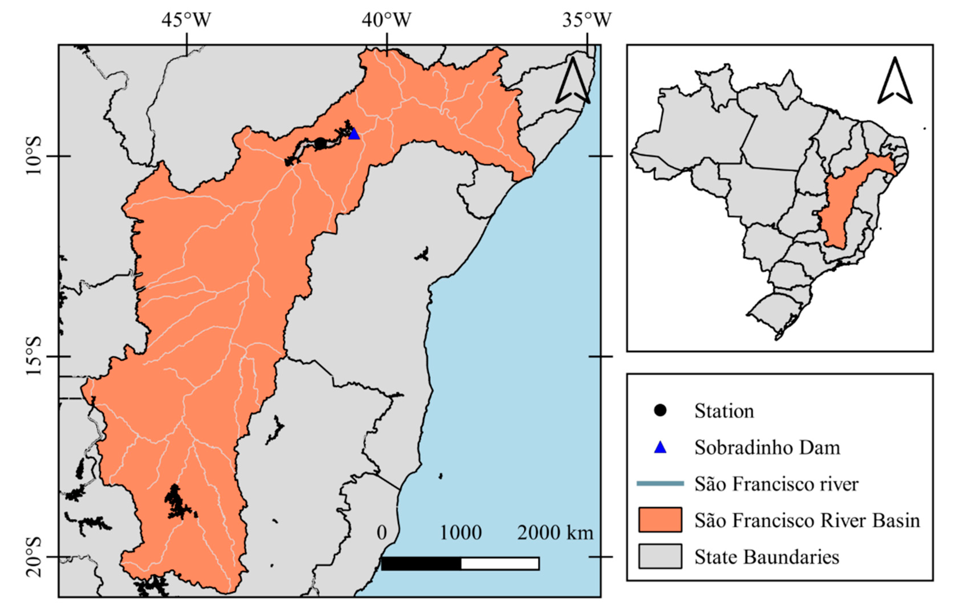
The Sobradinho reservoir is located in the São Francisco River Basin, Brazil (Figure 1). The basin has an area of approximately 639,219 km², equivalent to 8% of the country. It is the longest river that runs entirely in Brazilian territory. The São Francisco River runs through six Brazilian states (Minas Gerais, Goiás, Bahia, Pernambuco, Alagoas, and Sergipe) and the Federal District. The São Francisco River originates in Minas Gerais and runs 2863 km to the Atlantic Ocean [23].
The water and climate characteristics of the basin are highly variable. The Sobradinho reservoir presents critical periods of prolonged droughts due to low rainfall and high evapotranspiration. The rainfall season starts approximately in November and ends in April [23,24]. The average annual flow of the São Francisco River is 2846 m3/s, and, until 2013, the water withdrawn was 278 m³/s [25]. One of the uses of water resources in the São Francisco River is irrigation, whose withdrawal is 77% of the region’s total demand.
The São Francisco Region plays an essential role in generating electricity, with a potential installed in 2013 of 10,708 MW, coming from 28 small plants and 12 large plants (12% of the country’s total). The hydroelectric exploitation of the São Francisco River represents the NEB’s energy supply base [24]. There are several large dams along the São Francisco River, namely Três Marias, Sobradinho, Itaparica, Moxotó, Paulo Afonso I, II, III, and IV, and Xingó, which were constructed between 1962 (Três Marias) and 1994 (Xingó). The Sobradinho dam (coordinates: 9°25’49” S, 40°49’37” W; construction: 1973–1979; the beginning of operations: 1979–1982) is located 742 km from the mouth, in the Bahia state. The dam has a height of 41 m and length of 12.5 km. The reservoir has a maximum length of 320 km, a surface area of 4214 km², and a storage capacity of 34.1 × 10⁹ m³. The Sobradinho reservoir was built to achieve multiple uses such as multiannual flow regulation for hydropower, navigation, irrigation, and flood control management for the riverine communities of the São Francisco River Basin.
Monthly naturalized flows measured at a gauging station along the São Francisco River were obtained from the ONS. The naturalized flow of a hydroelectric plant is the flow that would be observed in that measurement gauge considering the river in its natural condition, that is, assuming that there is no reservoir regulating the flow and no human activity impacts. The streamflow time series range from January 1931 to December 2016 without any missing values. The gauge station is located approximately 95 km upstream of the Sobradinho dam. This station is likely to suffer minor effects of the Três Marias reservoir, the largest reservoir upstream of Sobradinho, and located about 1087 km from Sobradinho [4].
3. Materials and Methods
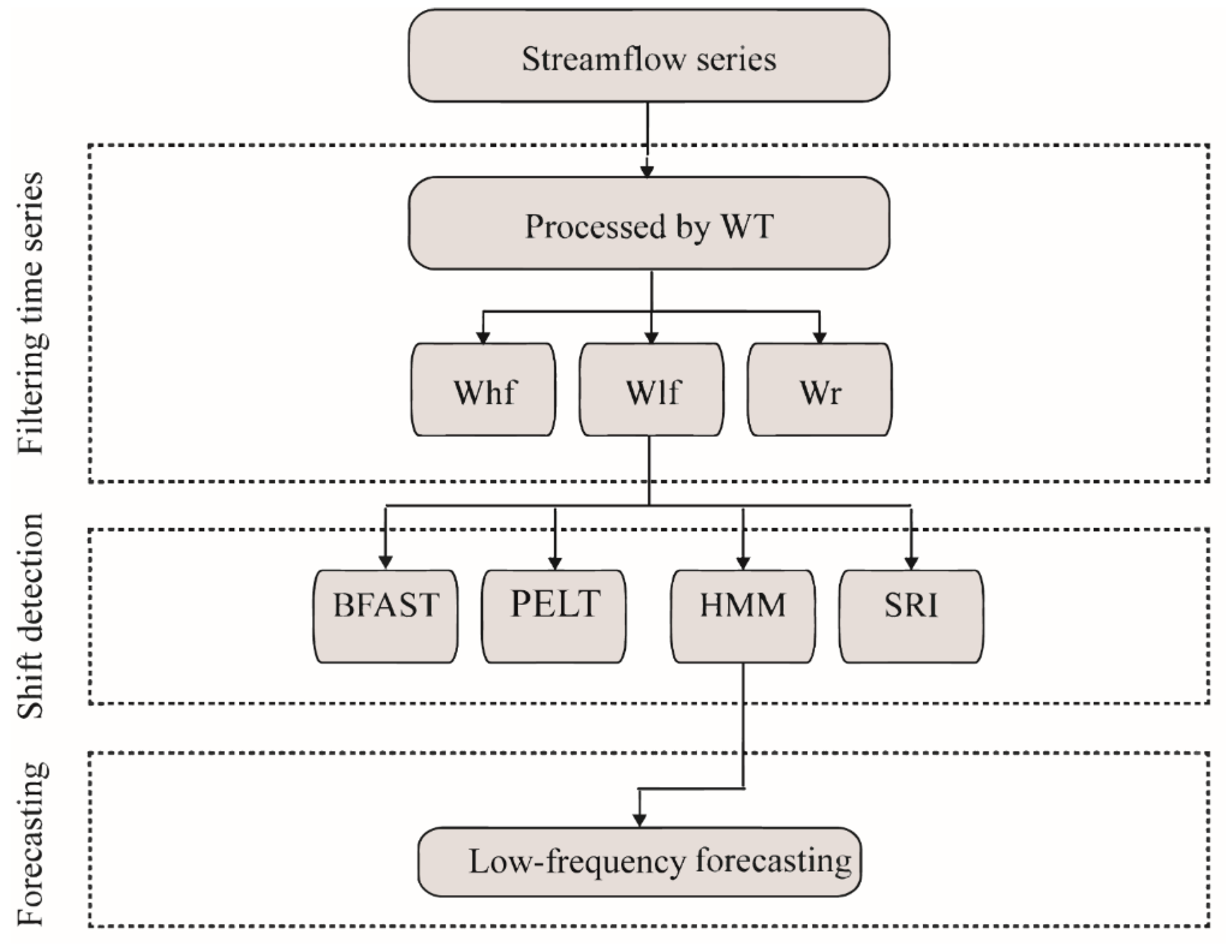
This section provides a brief description of the methods and the steps used for shift identification and projection of the low-frequency streamflow time series. All experiments were carried out in the R environment for statistical computing [26]. In this study, (i) the wavelet transform was used to decompose and reconstruct the low-frequency streamflow from the streamflow time series and (ii) a classical method (SRI) and three state-of-the-art methods (PELT, BFAST, and HMM) were used to identify the shifts in the low-frequency streamflow series. After the identification of the shifts present in the series and knowing how they repeated themselves, (iii) an HMM was used to project the low-frequency streamflow. The main advantage of applying this method to streamflow time series is its ability to simulate long persistence and regime-switching behavior [27]. Then, the degree of improvement in prediction accuracy from using the HMM as the projection method for low-frequency streamflow time series was assessed. Figure 2 illustrates the flowchart describing the key steps in this study.
3.1. Time Series Decomposition Using Wavelet Transform
An extensive method used in extracting the low-frequency part of a time series is the wavelet transform [28,29,30], which decomposes the series in the time-frequency domain and identifies the dominant modes of variability. A wavelet transform decomposes a time series into a set of functions, also known as the “daughter wavelet”, derived from the translation in time and scaling of the “mother wavelet”. The choice of the mother wavelet is a significant one, where the kind of wavelet transform chosen depends on the type of output information needed. There are many mother wavelet functions from which to choose, such as Haar wavelet, Daubechies wavelet, Mexican Hat wavelet, Morlet wavelet, and others. This study applied the Morlet wavelet, which is commonly used in hydrological time series because of its power to describe the time series adequately and provide a better time-frequency localization [31,32].
The signal component of the time series is identified by the 90–95% significance test using the white noise as a null hypothesis and the interpretation of the wavelet power spectrum. The identified significant component is then extracted from the original series using the reconstruction function. Reconstruction of the original time series over a set of periods can be obtained as follows:
where C is the reconstruction factor; and are the scale and time factor, respectively; is the factor that removes the energy scaling for the Morlet wavelet function; Re(Wave(s)) is the real part of the wavelet transform; and s is the scale parameter.
3.2. Regime Shift Detection
In this study, we applied the PELT algorithm and the HMM to detect shifts in the annual low-frequency streamflow time series, and the BFAST model and the SRI to detect shifts in the monthly low-frequency streamflow series.
3.2.1. SRI
Drought indices, such as SRI, are used for drought identification and the description of its intensity. The SRI is based on the concept of the Standardized Precipitation Index [34], discussed by the authors of [35]. Although the indices show similarities, the SRI incorporates hydrological processes that control the seasonal loss in streamflow due to the climate’s influence, thus being able to describe the hydrological aspects of droughts.
First, a long-term record was fitted to a probability distribution. A variety of probability distributions (e.g., gamma, lognormal, generalized extreme value, log-logistic, and generalized Pareto) have been used to fit monthly observations of different hydro-climatic variables for calculating drought indices [36,37]. Then, the cumulative distribution function (CDF) of the fitted marginal distribution was transformed into a standard normal variate Z.
After the low-frequency streamflow was decomposed and reconstructed using the wavelet transform to a significant variability frequency range, we tested three different distributions, where the best one was chosen to fit the reconstructed time series. The adjusted SRI (Ad-SRI), as we are calling the SRI of the low frequency, is not the same as the classical SRI as they present different information. Consequently, their variability range is different. The Ad-SRI uses the mean of a 12-month time scale to characterize the system’s state in that year. Afterward, the values are classified. Years with negative values were termed State 1 and years with positive values were termed State 2.
3.2.2. PELT Algorithm
The detection of breakpoints was based on the method presented in [38]. A data set is defined as being . In a model with multiple breakpoints (m) and their positions , each point is an integer between 1 and n − 1. It is defined that and . Consequently, the m breakpoints will split the data into m+1 segments. A common approach in the methodology to detect multiple breakpoints is to minimize the cost function as follows:
where C is a cost function for a segment, e.g., negative log-likelihood, and βf(m) is a penalty to guard against overfitting (a multiple breakpoint version of the threshold c).
Many breakpoints algorithms are implemented in the R package changepoint [39] used in this study, such as the binary segmentation algorithm, segmentation neighborhood, and the PELT algorithm [38]. The PELT shows speed gains and increased accuracy over the other methods. The method is an adaptation of the optimal partitioning, and for computational efficiency it removes points that can never be minima from the minimization performed at each iteration by the cost function [39]. We assessed the annual low-frequency streamflow with the PELT algorithm and divided the shifts into two states based on the breakpoint found by the algorithm. Negative values of low-frequency streamflow were termed State 1, whereas positive values were termed State 2.
3.2.3. BFAST
The BFAST method, proposed by the authors of [40], is a decomposition method that integrates the iterative decomposition of a time series into trend, seasonal, and remainder components to examine changes (i.e., trends and breakpoints) within the time series. The method has been applied to detect long-term seasonal changes in satellite image time series [40]. The general model is described as follows:
where is the observed data at time t, is the trend component, is the seasonal component and the remainder component denotes the remaining variation in the data beyond that in the seasonal and trend components.
Assuming that the entire time series has m breakpoints ,…, in the trend component , then the segment-specific slopes and intercepts can be calculated on each segment. The trend component can be expressed as follows:
where i = 1, …, m and we define = 0 and = n. The intercept and slope can be used to assess the magnitude and direction of the abrupt change.
Similarly, a harmonic model is applied to parameterize the seasonal component. The seasonal component is fixed between breakpoints. Given the time series has p seasonal breakpoints , …, , then the seasonal component can be calculated as follows:
where the unknown parameters are the segment-specific amplitude and phase , which must be estimated. The known frequency f is equal to 12 for the monthly observations used here. The moving sum test based on ordinary least squares residuals (OLS-MOSUM) is applied to detect whether one or more breakpoints occur [41]. The breakpoints are estimated using Bai and Perron’s method if the test indicates a significant change (p < 0.05). [42] argues that the Akaike information criterion (AIC) usually overestimates the number of breaks, and the Bayesian information criterion (BIC) is a more suitable procedure in many situations. Thus, in the method, the number of breaks was determined by the BIC, and the date and confidence interval of the date for each break were estimated. The BFAST model parameters were estimated by iterating the following steps:
Step 1: If the OLS-MOSUM test shows that breakpoints occur in the trend component, then the number and positions of the breakpoints in the trend component , …, are estimated through least squares from the seasonally adjusted data . For a specific segment, the trend component can be estimated by Equation (4). Then, the trend coefficient and are calculated for different segments using robust regression method based on M-estimation to account for potential outliers.
Step 2: Similarly, if the OLS-MOSUM test indicates that breakpoints occur in the seasonal component, then the number and positions of the breakpoints in the seasonal component , …, are estimated from the detrended data . The parameters and for each segment are calculated using a robust regression method based on M-estimation. We applied the BFAST model to monthly data and identified the shifts in the low-frequency streamflow.
3.2.4. HMM
HMM [43] is a statistical model in which the realizations from an unobserved Markov process represent the observed time series [44,45]. A Markov process is a random process whose future probabilities are determined by its most recent values. The HMM was developed for speech recognition and has been successfully used in many knowledge areas, including hydrology [27,44,46].
An HMM consists of state ( and observation variables. The distribution of can be written as and the marginal distribution for a discrete number of states can be described as mixture distribution with n components [45,46,47]. The equation is written as follows:
where , and () is the conditional distribution of the data.
The transition between states is governed by probabilities described as transition probabilities. They are denoted by the matrix , where the first row () has the probabilities from moving from state to . When dealing with the transition’s parameters in A, one must define the initial state or the prior probabilities π that define where the process begins.
The forward algorithm is used for calculating the joint likelihood [48]. The expectation–maximization algorithm is used to optimally estimate the parameters of the HMM. In this algorithm, the parameters are obtained with the maximization of the expected joint log-likelihood given the observations and states through an iterative process [45,49]. The Viterbi algorithm is applied to decode the observation sequences into hidden state sequences.
3.2.5. HMM for Projection
For the simulation of the model, the low-frequency streamflow was fitted to different HMMs, varying the number of hidden states. The model with the lowest BIC was chosen. Then, the model’s parameters were estimated, including the mean and standard deviation of each state and the transition matrix of the model.
The prediction method was based on the work proposed by the authors of [50], which is divided into three steps:
Step 1: The HMM parameters are calibrated using the training data, and the probability of the observed data is calculated.
Step 2: Based on similar data sets in the past data, we find parts of the training data with a similar likelihood.
Step 3: The difference between the streamflow of the previous year and the streamflow of the consecutive year is calculated to forecast the future streamflow.
When predicting the streamflow at a time step T + 1 of the time series, a part-time series of length D is chosen to be the training data, used to calibrate the HMM’s parameters, λ (π,A,B). Consequently, streamflow patterns similar to the current year are located in the past data. Considering that the predicted value must assume a similar pattern from the training data, the difference of a year’s streamflow and the next year’s value is calculated. The difference between years is estimated by the summation of the probability of being in a previous state multiplied by the mean of its respective states.
Similarly, to predict the streamflow at time T + 2, new training data is used by adding the predicted value and repeating the three-step-prediction process for the time step T + 2 and so on. Data length and quality are limitations in the method because shorter records cannot show the low-frequency variability efficiently needed in multidecadal projections.
3.2.6. Model Performance Metrics
The projection performance of the model for the low-frequency streamflow time series is estimated by comparing the observation and prediction. The root mean square error (RMSE), mean absolute error (MAE), and correlation coefficient (R) are used to estimate the performance of the HMM, as defined in Equations (8)–(10).
N is the number of input samples; and represent the observed and predicted runoff at time t, respectively; and and represent the averages of the observed and predicted runoff, respectively.
In the evaluation, the target values are R close to 1, MAE and RMSE close to 0. The RMSE is an ideal error index used to evaluate the global fitness of high streamflow values, whereas the MAE provides a more balanced measure of overall errors [22].
4. Results
4.1. Time Series Decomposition
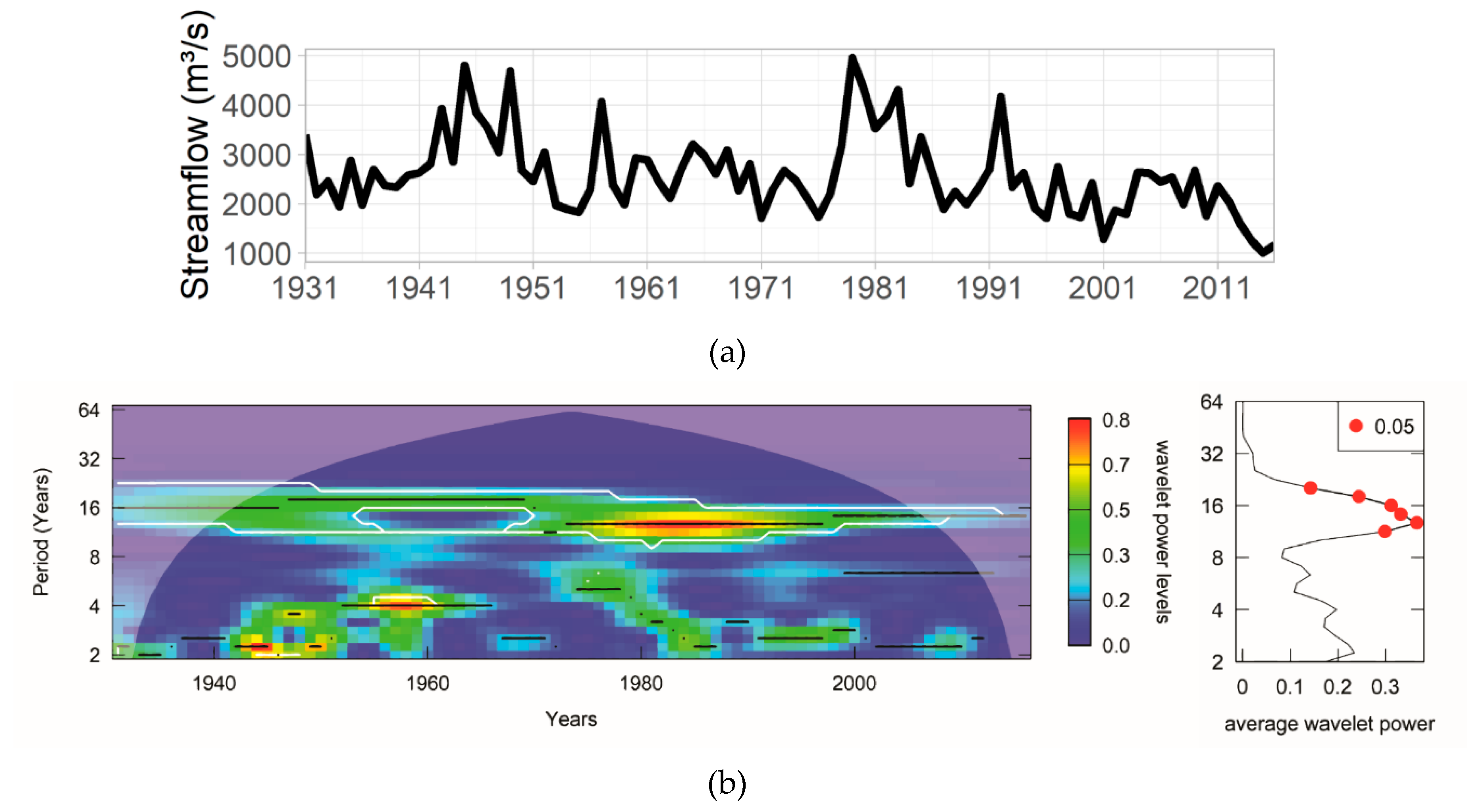
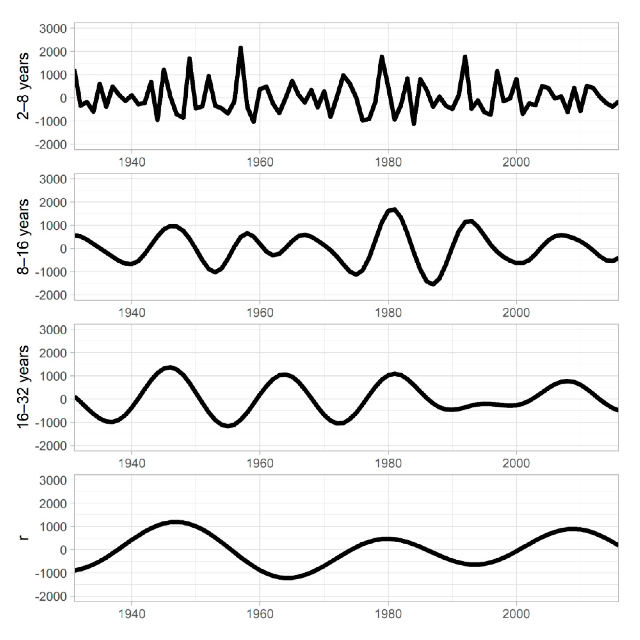
A wavelet transform is used to decompose and extract the low frequency from the time series of Sobradinho’s inflow. Figure 3a illustrates the annual streamflow time series, while Figure 3b shows the wavelet power spectrum and the average wavelet power over that period. The red points represent the significance levels and show which regions of the spectrum meet the significance level. The frequency chosen in this study was between 16 and 32 years since it presented significance in its power spectrum and the average wavelet power. The 16- to 32-year frequency represents 10.20% of the explained variance of the streamflow time series. Figure 4 illustrates the reconstructed time series using the wavelet transform decomposition. The series was reconstructed for high (2–8 years), medium (8–16 years), low (16–32 years) frequency, and the residue, which is represented with the frequency higher than 32 years.
4.2. Low-Frequency Streamflow Shift Detection
The identification of shifts in time series is still the subject of different methods that try to comprehend changes in hydrological records due to the effect of natural climatic variability and human activities. An analysis of the low-frequency streamflow time series was made using Ad-SRI, PELT, BFAST, and HMM, aiming to identify states in the time series.
In the Ad-SRI analysis, we tested three distributions (generalized Pareto, Pearson type III, and gamma), and the best fit for the low-frequency streamflow was Pearson type III. The Pearson type III distribution has also been widely used for flow frequency analyses [51]. Although the authors of [51] reported an excessive frequency of negative values, the analyzed low-frequency streamflow seems to present bias for positive values. The BFAST was also used to assess the shifts in a monthly time frame. The model did not present any seasonal breakpoints, only trend breakpoints. The PELT algorithm and the HMM with two states were applied to evaluate the low-frequency streamflow annually. Figure 5 illustrates the shifts in the low-frequency streamflow dynamics.
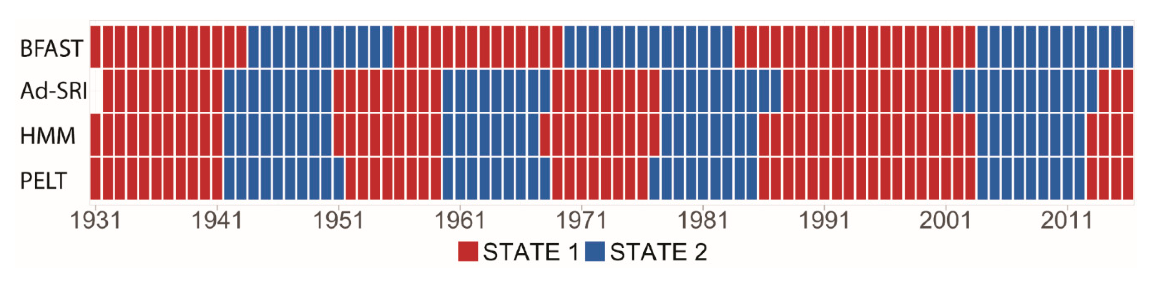
Figure 5 shows that the classification of the Ad-SRI, HMM, and PELT were very similar, presenting a cycling behavior of seven to nine years duration up until the mid-1980s. In that period, State 1 of the Ad-SRI model started later compared with the PELT and the HMM. The BFAST classification produced longer cycles, of approximately 11 to 16 years, compared with the other models in this study.
The first shift from State 1 to State 2 occurred in the beginning of the 1950s for most models, whereas for the BFAST it started five years later and lasted for approximately three years more than the other models. The BFAST showed a similar classification as the other models from 1985 onward.
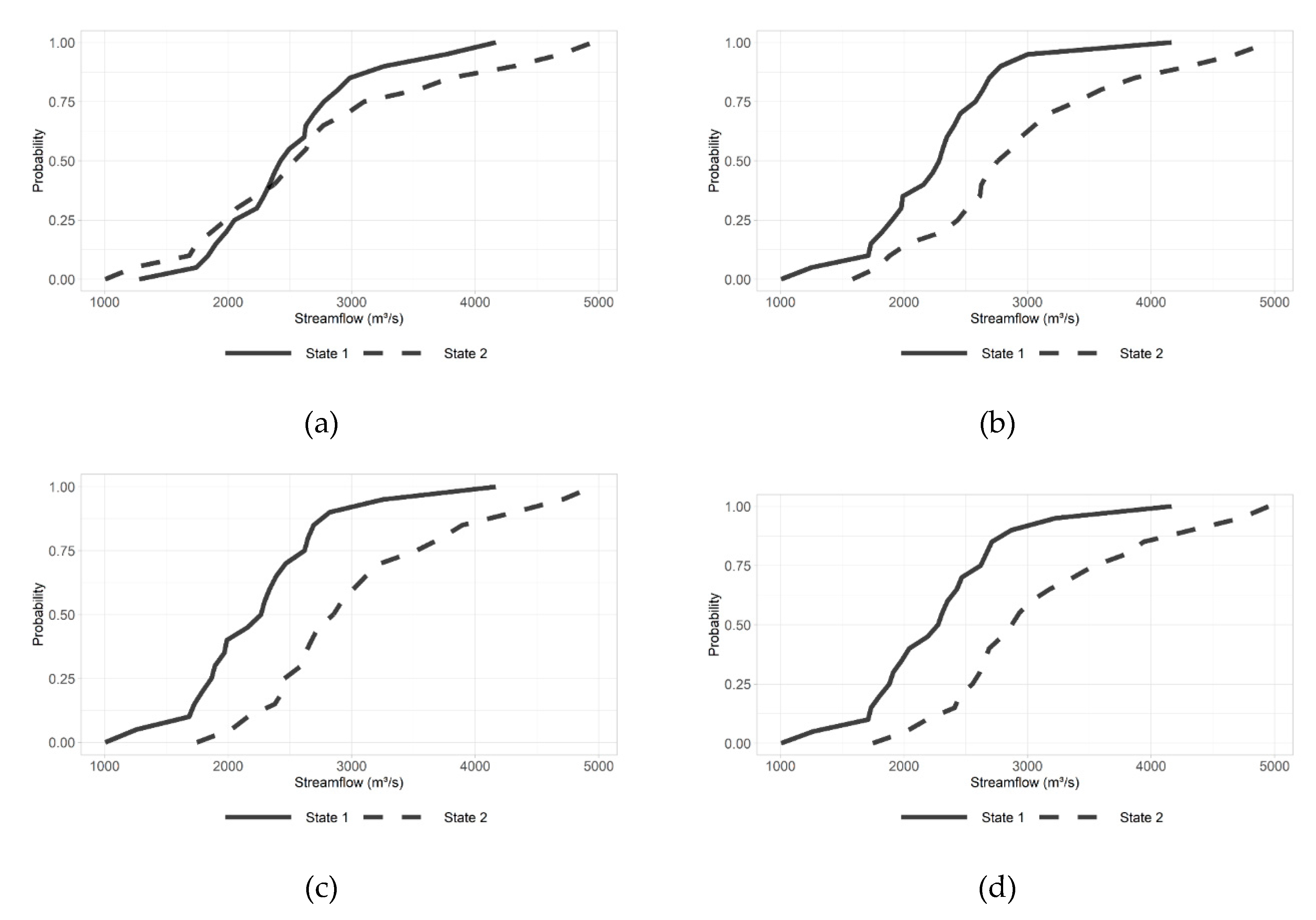
The low-frequency streamflow shift models showed a clear separation of the states. Then, the CDF for each state was calculated using the series’ data without being decomposed by the wavelet transform to verify if those periods followed a similar statistical distribution.
Figure 6 illustrates that the two states of the series without being decomposed by the wavelet transform do not follow the same distribution in the CDF plot. When comparing the CDFs across the four methods, the BFAST is unable to distinguish states well. Results of the Ad-SRI, PELT, and HMM were similar. State 2 presented a probability of higher streamflow values than in State 1 in all models. Hence, the wet periods have a higher likelihood of occurring than the dry periods. The low frequency shows a clear effect in the pattern of the time series, which justifies its study as one of the influencing components of the time series behavior. Knowing that the states have a different probability distribution and identifying the states in which the system presents itself give the modeler great insight on how to project the time series.
4.3. Projection of the Low-Frequency Streamflow with the HMM
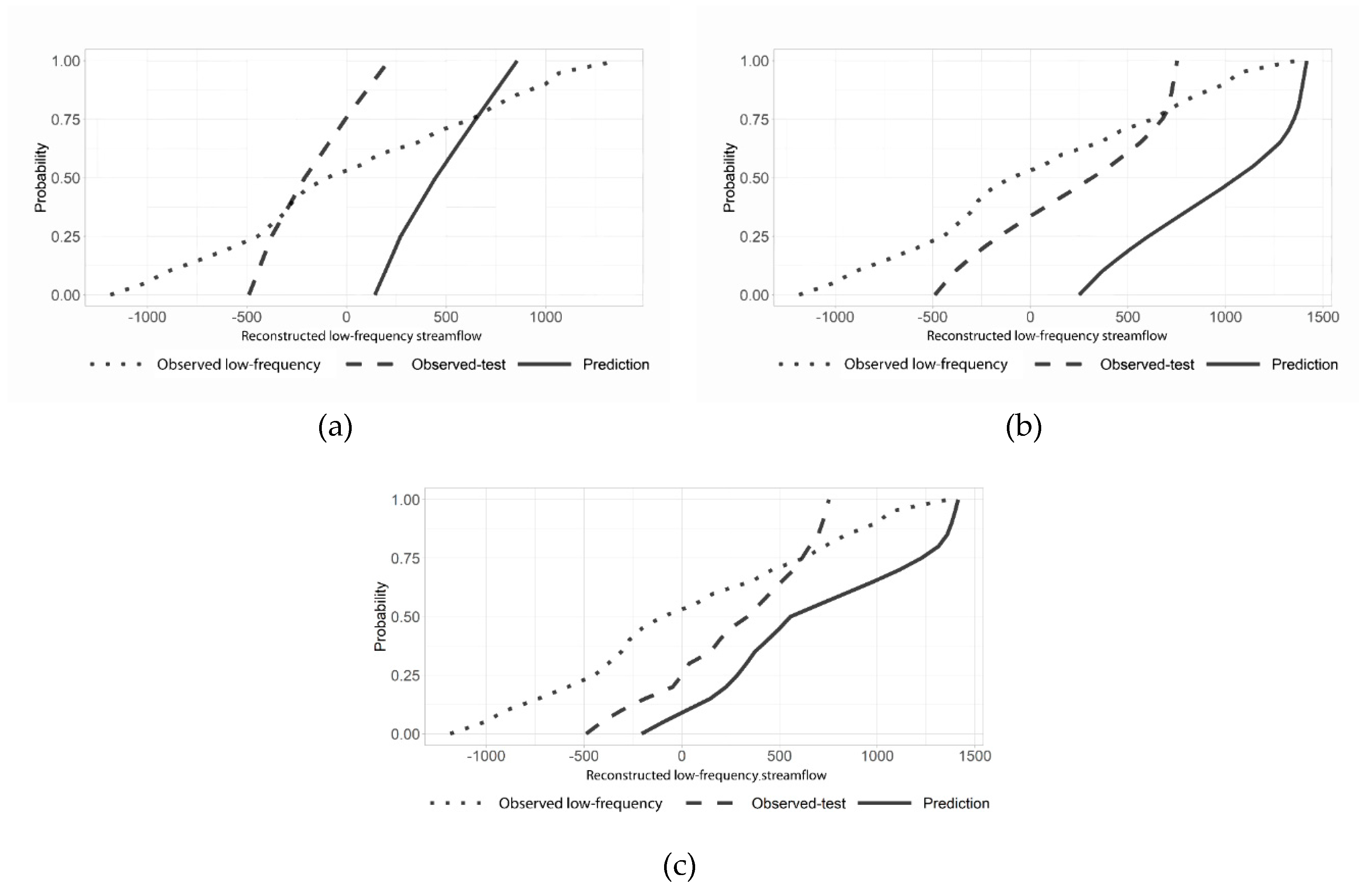
The method applied to predict the low-frequency streamflow time series of the Sobradinho reservoir was based on the work proposed by the authors of [50]. In this case, the lowest BIC was the criterion for the number of states in the HMM. The model was used to predict periods of 5, 10, and 15 years. Figure 7 shows the CDFs of the predicted low-frequency streamflow, observed low-frequency streamflow for the test period, and the observed low-frequency streamflow from 1931 to 2016 in the (a) 5-year, (b) 10-year, and (c) 15-year projection.
Although the models overestimated the low-frequency streamflow values, they were able to accompany the shifts in the streamflow regime. Compared with the mean of the training periods (1931–2012, 1931–2007, and 1931–2001), the models were able to follow the dry and wet periods better than the mean values. Figure 7 presents an improvement in the information of the dry period. Low-frequency streamflow (1931–2016) has a high probability of average low flow than the observed-test, and the model prediction can model this behavior. The entire time series (observed low-frequency streamflow from 1931 to 2016) presents a variance that is greater than the observation. The model prediction has the same scale as the variance of observation of the test period.
Table 1 shows the statistical accuracy of the predictions by different models, indicated by RMSE, MAE, and R. Smaller values of RMSE and MAE suggest more accurate predictions. High values of R indicate a better fit between prediction and observation. Table 1 shows that the period of 15 years had the lowest RMSE and MAE. However, it presented the lowest value of R as well. The RMSE and MAE values are still close to those of 5 years and 10 years, with an increase of 8% and 17%, respectively, for the RMSE. Furthermore, there was a decrease of 63% for the R in the 15-year period compared with the other projections.
5. Discussion and Conclusions
The nonlinearity of hydrological systems has been recognized for many years. The recent development of computational power and data acquisition provided us with tools and new methods to study temporal and spatial variability in hydrological variables [20]. Different studies [4,20] provided evidence that the time series of the Sobradinho reservoir presents nonlinear behavior, particularly after its construction. Therefore, the wavelet transform was applied in this paper as a pre-processing tool to extract significant features such as the low-frequency variability and to gain insight into time-varying characteristics that the streamflow time series may present.
Previous studies have indicated that a hydrological regime shift may occur due to anthropogenic activities, such as dam construction. In this context, the analysis of the low-frequency streamflow using the BFAST model showed a shift in 1986, and for the other models, the shift started in 1985. We also observed a reduction in the low-frequency streamflow peaks from 1985. These alterations in the low-frequency streamflow regime might indicate the influence on the river regime of the Sobradinho dam, which was constructed between 1973 and 1979 and started functioning between 1979 and 1982. According to the authors of [52], downstream areas of the Sobradinho dam presented significant changes in the annual seasonality of floods. Although more events that contributed to increases in precipitation occurred during the 1986–2006 period, this was not reflected in the flood data, concluding that dam impacts combined with other water withdrawals, particularly for agriculture, are the main reasons for changes in floods along the São Francisco River [52]. Other concerns raised for the region are the increase in the amount of water removed from the São Francisco River due to the increase in irrigation farming and illegal water removal from the river [53]. These anthropogenic actions are tough to measure and carry a great impact on flow rates.
Some authors [54,55] observed a systematic change in the hydrological time series of the NEB in the late 1970s and early 1980s that are associated with the natural fluctuations such as decadal variability. Several studies point out that precipitation records over South America exhibit decadal and interdecadal variability. This precipitation variability has been associated with sea surface temperature (SST) anomalies such as the PDO [20,56] and the AMO [57] in the NEB. Thus, although there was no apparent correlation between the climate indices and the analyzed low-frequency streamflow, these variables may influence some periods of the low-frequency streamflow behavior and the shifts present in hydrological variables.
Another significant perturbation that can cause changes in the hydrological system is extreme events such as droughts. The recent intensive drought developed in the NEB region for the period 2010–2017 has been one of the worst in the last decades. We can see an apparent decrease in low-frequency streamflow. However, in the low-frequency streamflow, the decrease is not that intense. That phenomenon may be because the drought was associated with the strong 2015–2016 El Niño, which brought warmer weather and SSTs [58]. That influence may be present in the high frequency of the time series (2- to 8-year frequency in Figure 4).
Future projections state that temperatures in the NEB should increase, while rainfall could decline by approximately 25–50% in semi-arid areas. Consequently, flow rates will be reduced for various rivers in the NEB [58,59]. Hydroelectric potential in the São Francisco River Basin will be reduced due to more frequent and intense climate-induced droughts. Water allocation and appropriate land management are necessary for the region [52]. Consequently, more realistic projections can help to improve water management in the region.
In this study, we also proposed a model to forecast the nonlinear low-frequency streamflow series. Three scenarios of projection were modeled and evaluated using three statistical performance evaluation measures (RMSE, MAE, and R). The forecasts for 5- and 10-year periods presented remarkably high values of R. Although the value for the 15-year period was low, the result is significant when compared with the results provided in [7], whose authors used a climate hidden Markov model and presented an R² of approximately 0.26 for a lead time of 15 years. The model presents an improvement in the information of the dry period. Low-frequency streamflow (1931–2016) has a higher probability of average low flow than the test data set, and the model prediction can capture this behavior. This information is relevant for water resource planning, in particular for drought planning. Furthermore, as extreme climatic events become more frequent and threatening, it is essential to assess watersheds and prepare strategies for those situations.
Identifying different state periods also reveals the impact of low frequency in the streamflow time series. Due to the clear separation of states in the analysis, we observed that the patterns have different probability distributions through the CDF plots; thus, the low-frequency variability conditions the flows of a given year. The model comparison in this paper provides an insight into a modified version of a classical method such as the SRI and state-of-the-art methods such as BFAST, PELT, and HMM available for identifying shifts in the time series. Assessing the current state of low-frequency streamflow allows the assessment of the dynamic risk of extreme events and an accurate forecast of streamflow. The HMM forecast model is a tool to aid in the management and operation of this reservoir.
Author Contributions
Conceptualization, F.d.A.d.S.F.; Data curation, L.Z.R.R.; Formal analysis, L.Z.R.R. and F.d.A.d.S.F.; Funding acquisition, F.d.A.d.S.F.; Investigation, L.Z.R.R.; Methodology, F.d.A.d.S.F.; Resources, F.d.A.d.S.F.; Software, L.Z.R.R.; Supervision, F.d.A.d.S.F.; Writing—original draft, L.Z.R.R.; Writing—review and editing, L.Z.R.R. and F.d.A.d.S.F. All authors have read and agreed to the published version of the manuscript.
Funding
This research was funded by the Conselho Nacional de Desenvolvimento Científico e Tecnológico—Brasil (CNPq), grant number 441457/2017-7 (NEXUS project).
Acknowledgments
The authors thankfully acknowledge the support for this research provided by the Coordenação de Aperfeiçoamento de Pessoal de Nível Superior - Brasil (CAPES) and the Conselho Nacional de Desenvolvimento Científico e Tecnológico - Brasil (CNPq). They would also like to thank the Fundação Cearense de Apoio Científico e Tecnológico (FUNCAP) for its support under the Cientista Chefe program.
Conflicts of Interest
The authors declare no conflict of interest.
References
- Wang, F.; Zhao, G.; Mu, X.; Gao, P.; Sun, W. Regime Shift Identification of Runoff and Sediment Loads in the Yellow River Basin, China. Water 2014, 6, 3012–3032. [Google Scholar] [CrossRef] [Green Version]
- IPCC, Intergovernmental Panel on Climate Change. In Climate Chang. 2007: Impacts, Adaptation and Vulnerability; Cambridge University Press: Cambridge, UK, 2007.
- Zhao, G.; Li, E.; Mu, X.; Rayburg, S.; Tian, P. Changing Trends and Regime Shift of Streamflow in the Yellow River Basin. Stoch Environ. Res. Risk Assess. 2015, 29, 1331–1343. [Google Scholar] [CrossRef]
- Barreto, I.D.C.; Xavier Junior, S.F.A.; Stosic, T. Long-Term Correlations in São Francisco River Flow: The Influence of Sobradinho Dam. Rev. Bras. Meteorol. 2019, 34, 293–300. [Google Scholar] [CrossRef] [Green Version]
- Kwon, H.-H.; Lall, U.; Khalil, A.F. Stochastic Simulation Model for Nonstationary Time Series Using an Autoregressive Wavelet Decomposition: Applications to Rainfall and Temperature. Water Resour. Res. 2007, 43, 5662–5675. [Google Scholar] [CrossRef]
- Cheng, L.; AghaKouchak, A. Nonstationary Precipitation Intensity-Duration-Frequency Curves for Infrastructure Design in a Changing Climate. Sci. Rep. 2015, 4, 7093. [Google Scholar] [CrossRef] [Green Version]
- Erkyihun, S.; Zagona, E.; Rajagopalan, B. Wavelet and Hidden Markov-Based Stochastic Simulation Methods Comparison on Colorado River Streamflow. J. Hydrol. Eng. 2017, 22, 04017033. [Google Scholar] [CrossRef]
- Milly, P.C.D.; Betancourt, J.; Falkenmark, M.; Hirsch, R.M.; Kundzewicz, Z.W.; Lettenmaier, D.P.; Stouffer, R.J. Stationarity is Dead: Whither Water Management? Science 2008, 319, 573–574. [Google Scholar] [CrossRef] [PubMed]
- Salas, J.D.; Obeysekera, J. Revisiting the Concepts of Return Period and Risk for Nonstationary Hydrologic Extreme Events. J. Hydrol. Eng. 2014, 19, 554–568. [Google Scholar] [CrossRef] [Green Version]
- Garreaud, R.D.; Vuille, M.; Compagnucci, R.; Marengo, J. Present-Day South American Climate. Palaeogeogr. Palaeoclimatol. Palaeoecol. 2009, 281, 180–195. [Google Scholar] [CrossRef]
- Hodson, D.L.R.; Sutton, R.T.; Cassou, C.; Keenlyside, N.; Okumura, Y.; Zhou, T. Climate Impacts of Recent Multidecadal Changes in Atlantic Ocean Sea Surface Temperature: A Multimodel Comparison. Clim. Dyn. 2010, 34, 1041–1058. [Google Scholar] [CrossRef] [Green Version]
- Burn, D.H.; Hag Elnur, M.A. Detection of Hydrologic Trends and Variability. J. Hydrol. 2002, 255, 107–122. [Google Scholar] [CrossRef]
- da Silva Silveira, C.; Alexandre, A.M.B.; de Souza Filho, F.d.A.; Vasconcelos Junior, F.d.C.V.; Cabral, S.L. Monthly Streamflow Forecast for National Interconnected System (NIS) using Periodic Auto-Regressive Endogenous Models (PAR) and Exogenous (PARX) with Climate Information. RBRH 2017, 22, e30. [Google Scholar] [CrossRef] [Green Version]
- Tang, Q.; Oki, T.; Dai, A. Historical and Future Changes in Streamflow and Continental Runoff. In Terrestrial Water Cycle and Climate Change: Natural and Human-Induced Impacts; American Geophysical Union: Hoboken, NJ, USA, 2016; pp. 17–37. [Google Scholar] [CrossRef]
- Marengo, J.A.; Tomasella, J.; Uvo, C.R. Trends in Streamflow and Rainfall in Tropical South America: Amazonia, Eastern Brazil, and Northwestern Peru. J. Geophys. Res. Atmos. 1998, 103, 1775–1783. [Google Scholar] [CrossRef]
- Milly, P.C.D.; Dunne, K.A.; Vecchia, A.V. Global Pattern of Trends in Streamflow and Water Availability in a Changing Climate. Nature 2005, 438, 347–350. [Google Scholar] [CrossRef]
- Grimm, A.M.; Saboia, J.P.J. Interdecadal Variability of the South American Precipitation in the Monsoon Season. J. Clim. 2015, 28, 755–775. [Google Scholar] [CrossRef]
- Jain, S.; Lall, U. Magnitude and Timing of Annual Maximum Floods: Trends and Large-Scale Climatic Associations for the Blacksmith Fork River, Utah. Water Resour. Res. 2000, 36, 3641–3651. [Google Scholar] [CrossRef]
- Oliveira, V.G.; LIMA, C.H.R. Multiscale Streamflow Forecasts for the Brazilian Hydropower System using Bayesian Model Averaging (BMA). RBRH 2016, 21, 618–635. [Google Scholar] [CrossRef] [Green Version]
- Stosic, T.; Telesca, L.; Ferreira, D.V.S.; Stosic, B. Investigating Anthropically Induced Effects in Streamflow Dynamics by using Permutation Entropy and Statistical Complexity Analysis: A Case Study. J. Hydrol. 2016, 540, 1136–1145. [Google Scholar] [CrossRef]
- Luiz Silva, W.; Xavier, L.N.R.; Maceira, M.E.P.; Rotunno, O.C. Climatological and Hydrological Patterns and Verified Trends in precipitation and Streamflow in the Basins of Brazilian Hydroelectric Plants. Theor. Appl. Climatol. 2019, 137, 353–371. [Google Scholar] [CrossRef]
- Wang, Z.; Qiu, J.; Li, F. Hybrid Models Combining EMD/EEMD and ARIMA for Long-Term Streamflow Forecasting. Water 2018, 10, 853. [Google Scholar] [CrossRef] [Green Version]
- ANA. Plano de Recursos Hídricos da Bacia do Rio São Francisco. 2016. Available online: https://cbhsaofrancisco.org.br/plano-de-recursos-hidricos-da-bacia-hidrografica-do-rio-sao-francisco/ (accessed on 13 January 2020).
- Mendes, L.A.; de Barros, M.T.L.; Zambon, R.C.; Yeh, W.W.-G. Trade-Off Analysis among Multiple Water Uses in a Hydropower System: Case of São Francisco River Basin, Brazil. J. Water Resour. Plan. Manag. 2015, 141, 04015014. [Google Scholar] [CrossRef]
- ANA. Conjuntura dos recursos hídricos no Brasil: Regiões hidrográficas do Brasil. 2013. Available online: https://goo.gl/P87Msi (accessed on 13 January 2020).
- R Development Core Team. R: A Language and Environment for Statistical Computing. R Version 3.5.2 (2018); R Foundation for Statistical Computing: Vienna, Austria, 2018; Available online: https://www.r-project.org/.
- Bracken, C.; Rajagopalan, B.; Zagona, E. A Hidden Markov Model Combined with Climate Indices for Multidecadal Streamflow Simulation. Water Resour. Res. 2014, 50, 7836–7846. [Google Scholar] [CrossRef]
- Labat, D. Recent Advances in Wavelet Analyses: Part 1. A Review of Concepts. J. Hydrol. 2005, 314, 275–288. [Google Scholar] [CrossRef]
- Nourani, V.; Baghanam, A.H.; Adamowski, J.; Gebremichael, M. Using Self-Organizing Maps and Wavelet Transforms for Space–Time Pre-Processing of Satellite Precipitation and Runoff Data in neural Network Based Rainfall–Runoff Modeling. J. Hydrol. 2013, 476, 228–243. [Google Scholar] [CrossRef]
- Torrence, C.; Compo, G.P. A Practical Guide to Wavelet Analysis. Bull. Am. Meteorol. Soc. 1998, 79, 61–78. [Google Scholar] [CrossRef] [Green Version]
- Huo, X.; Lei, L.; Liu, Z.; Hao, Y.; Hu, B.X.; Zhan, H. Application of Wavelet Coherence Method to Investigate Karst Spring Discharge Response to Climate Teleconnection Patterns. JAWRA J. Am. Water Resour. Assoc. 2016, 52, 1281–1296. [Google Scholar] [CrossRef]
- Nalley, D.; Adamowski, J.; Khalil, B.; Biswas, A. Inter-Annual to Inter-Decadal Streamflow Variability in Quebec and Ontario in Relation to Dominant Large-Scale Climate Indices. J. Hydrol. 2016, 536, 426–446. [Google Scholar] [CrossRef]
- Rosch, A.; Schmidbauer, H. WaveletComp 1.1: A Guided Tour through the R Package. 2016. Available online: https://CRAN.R-project.org/package=WaveletComp (accessed on 18 February 2020).
- McKee, T.B.; Doesken, N.J.; Kleist, J. The Relationship of Drought Frequency and Duration to Time Scales. In Proceedings of the 8th Conference on Applied Climatology; American Meteorological Society: Boston, MA, USA, 1993; pp. 179–183. [Google Scholar]
- Shukla, S.; Wood, A.W. Use of a Standardized Runoff Index for Characterizing Hydrologic Drought. Geophys. Res. Lett. 2008, 35, L02405. [Google Scholar] [CrossRef] [Green Version]
- Vicente-Serrano, S.M.; Beguería, S.; López-Moreno, J.I. A Multiscalar Drought Index Sensitive to Global Warming: The Standardized Precipitation Evapotranspiration Index. J. Clim. 2010, 23, 1696–1718. [Google Scholar] [CrossRef] [Green Version]
- Stagge, J.H.; Tallaksen, L.M.; Gudmundsson, L.; Van Loon, A.F.; Stahl, K. Candidate Distributions for Climatological Drought Indices (SPI and SPEI). Int. J. Climatol. 2015, 35, 4027–4040. [Google Scholar] [CrossRef]
- Killick, R.; Fearnhead, P.; Eckley, I.A. Optimal Detection of Changepoints with a Linear Computational Cost. J. Am. Stat. Assoc. 2012, 107, 1590–1598. [Google Scholar] [CrossRef]
- Killick, R.; Eckley, I.A. Changepoint: An R Package for Changepoint Analysis. J. Stat. Softw. 2014, 58. [Google Scholar] [CrossRef] [Green Version]
- Verbesselt, J.; Hyndman, R.; Newnham, G.; Culvenor, D. Detecting Trend and Seasonal Changes in Satellite Image Time Series. Remote Sens. Environ. 2010, 114, 106–115. [Google Scholar] [CrossRef]
- Bai, J.S.; Perron, P. Estimating and Testing Linear Models with Multiple Structural Changes. Econometrica 1998, 66, 47–78. [Google Scholar] [CrossRef]
- Bai, J.S.; Perron, P. Computation and Analysis of Multiple Structural Change Models. JAE 2003, 18, 1–22. [Google Scholar] [CrossRef] [Green Version]
- Rabiner, L.R. A Tutorial on Hidden Markov Models and Selected Applications in Speech Recognition. Proc. IEEE 1989, 77, 257–286. [Google Scholar] [CrossRef]
- Mallya, G.; Tripathi, S.; Kirshner, S.; Govindaraju, R.S. Probabilistic Assessment of Drought Characteristics Using Hidden Markov Model. J. Hydrol. Eng. 2013, 18, 834–845. [Google Scholar] [CrossRef] [Green Version]
- Zucchini, W.; MacDonald, I.L.; Langrock, R. Hidden Markov Models for Time Series, 2nd ed.; Chapman and Hall/CRC: New York, NY, USA, 2016. [Google Scholar]
- Liu, Y.; Ye, L.; Qin, H.; Hong, X.; Ye, J.; Yin, X. Monthly Streamflow Forecasting Based on Hidden Markov Model and Gaussian Mixture Regression. J. Hydrol. 2018, 561, 146–159. [Google Scholar] [CrossRef]
- Visser, I. Seven Things to Remember about Hidden Markov Models: A Tutorial on Markovian Models for Time Series. J. Math. Psychol. 2011, 55, 403–415. [Google Scholar] [CrossRef]
- Lystig, T.C.; Hughes, J.P. Exact Computation of the Observed Information Matrix for Hidden Markov Models. J. Comput. Graph. Stat. 2002, 11, 678–689. [Google Scholar] [CrossRef]
- Baum, L.E.; Petrie, T. Statistical Inference for Probabilistic Functions of Finite State Markov Chains. Ann. Math. Stat. 1966, 37, 1554–1563. [Google Scholar] [CrossRef]
- Hassan, M.R.; Nath, B. Stock Market Forecasting using Hidden Markov Model: A New Approach. In Proceedings of the 5th International Conference on Intelligent Systems Design and Applications (ISDA’05), Warsaw, Poland, 8–10 September 2005; pp. 192–196. [Google Scholar] [CrossRef]
- Vicente-Serrano, S.M.; López-Moreno, J.I.; Beguería, S.; Lorenzo-Lacruz, J.; Azorin-Molina, C.; Morán-Tejeda, E. Accurate Computation of a Streamflow Drought Index. J. Hydrol. Eng. 2012, 17, 318–332. [Google Scholar] [CrossRef] [Green Version]
- Santos, H.D.A.; dos Santos, P.P.; Kenji, D.O.L. Changes in the Flood Regime of São Francisco River (Brazil) from 1940 to 2006. Reg. Environ. Change 2012, 12, 123–132. [Google Scholar] [CrossRef]
- De Jong, P.; Tanajura, C.A.S.; Sánchez, A.S.; Dargaville, R.; Kiperstok, A.; Torres, E.A. Hydroelectric Production from Brazil’s São Francisco River Could Cease Due to Climate Change and Inter-Annual Variability. Sci. Total Environ. 2018, 634, 1540–1553. [Google Scholar] [CrossRef] [PubMed]
- Marengo, J.A.; Valverde, M.C. Caracterização do Clima no Século XX e Cenário de Mudanças de Clima para o Brasil no Século XXI Usando os Modelos do IPCC-AR4. Rev. Multiciência 2007, 8, 5–28. [Google Scholar]
- Alves, B.C.C.; Souza Filho, F.A.; Silveira, C.S. Análise de Tendências e Padrões de Variação das séries Históricas de Vazões do Operador Nacional do Sistema (ONS). RBRH 2013, 18, 19–34. [Google Scholar] [CrossRef]
- Kayano, M.T.; Andreoli, R.V. Relations of South American Summer Rainfall Interannual Variations with the Pacific Decadal Oscillation. Int. J. Climatol. 2007, 27, 531–540. [Google Scholar] [CrossRef]
- Knight, J.R.; Folland, C.K.; Scaife, A.A. Climate Impacts of the Atlantic Multidecadal Oscillation. Geophys. Res. Lett. 2006, 33, 1610–1625. [Google Scholar] [CrossRef] [Green Version]
- Marengo, J.A.; Torres, R.R.; Alves, L.M. Drought in Northeast Brazil—Past, Present, and Future. Theor. Appl. Climatol. 2017, 129, 1189–1200. [Google Scholar] [CrossRef]
- Tanajura, C.A.S.; Genz, F.; Araújo, H.A. Mudanças Climáticas e Recursos Hídricos na Bahia: Validação da Simulação do Clima Presente do HadRM3P e Comparação com os Cenários A2 e B2 para 2070–2100. Rev. Bras. Meteor. 2010, 25, 345–358. [Google Scholar] [CrossRef] [Green Version]
Figure 1.
Location of the Sobradinho Reservoir, Brazil.

Figure 2.
Flowchart of the procedure applied in the study describing the steps of the shift detection and projection model. The time series is filtered using wavelet transform (WT) into the high-frequency (Whf), low-frequency (Wlf), and residue (Wr) components.
Figure 2.
Flowchart of the procedure applied in the study describing the steps of the shift detection and projection model. The time series is filtered using wavelet transform (WT) into the high-frequency (Whf), low-frequency (Wlf), and residue (Wr) components.

Figure 3.
(a) Annual streamflow time series of the Sobradinho reservoir; (b) the wavelet power spectrum and the average wavelet power over that period.
Figure 3.
(a) Annual streamflow time series of the Sobradinho reservoir; (b) the wavelet power spectrum and the average wavelet power over that period.

Figure 4.
The reconstructed time series of the wavelet transforms decomposition. The y-axis represents the different frequencies selected for a band-pass filter of wavelets for the reconstruction of the time series. The first series is the high-frequency (2–8 years), next is the medium-frequency (8–16 years), followed by the low-frequency (16–32 years) and the residue, which is the frequency higher than 32 years.

Figure 5.
Comparison of the state classification methodologies for low-frequency variability. The first line is the identification using the breaks for additive seasonal and trend (BFAST) method, then the Standardized Runoff Index (SRI), followed by the Pruned Exact Linear Time (PELT) algorithm, and two-state hidden Markov model (HMM) classification.

Figure 6.
The cumulative distribution functions (CDFs) of the series without being decomposed by the wavelet transform for the state classification using (a) BFAST, (b) adjusted SRI (Ad-SRI), (c) PELT, and (d) HMM.
Figure 6.
The cumulative distribution functions (CDFs) of the series without being decomposed by the wavelet transform for the state classification using (a) BFAST, (b) adjusted SRI (Ad-SRI), (c) PELT, and (d) HMM.

Figure 7.
The CDFs of the predicted low-frequency streamflow, observed low-frequency streamflow for the test period, and the observed low-frequency streamflow from 1931 to 2016 in the (a) 5-year, (b) 10-year, and (c) 15-year projection.
Figure 7.
The CDFs of the predicted low-frequency streamflow, observed low-frequency streamflow for the test period, and the observed low-frequency streamflow from 1931 to 2016 in the (a) 5-year, (b) 10-year, and (c) 15-year projection.


Table 1.
Statistical results of the predictive accuracy.
| Projection Period | RMSE | MAE | R |
|---|---|---|---|
| 5 years | 647.24 | 647.18 | 0.99 |
| 10 years | 722.57 | 721.35 | 0.99 |
| 15 years | 599.83 | 545.08 | 0.36 |
© 2020 by the authors. Licensee MDPI, Basel, Switzerland. This article is an open access article distributed under the terms and conditions of the Creative Commons Attribution (CC BY) license (http://creativecommons.org/licenses/by/4.0/).
Share and Cite
MDPI and ACS Style
Rolim, L.Z.R.; de Souza Filho, F.d.A. Shift Detection in Hydrological Regimes and Pluriannual Low-Frequency Streamflow Forecasting Using the Hidden Markov Model. Water 2020, 12, 2058. https://0-doi-org.brum.beds.ac.uk/10.3390/w12072058
AMA Style
Rolim LZR, de Souza Filho FdA. Shift Detection in Hydrological Regimes and Pluriannual Low-Frequency Streamflow Forecasting Using the Hidden Markov Model. Water. 2020; 12(7):2058. https://0-doi-org.brum.beds.ac.uk/10.3390/w12072058
Chicago/Turabian StyleRolim, Larissa Zaira Rafael, and Francisco de Assis de Souza Filho. 2020. "Shift Detection in Hydrological Regimes and Pluriannual Low-Frequency Streamflow Forecasting Using the Hidden Markov Model" Water 12, no. 7: 2058. https://0-doi-org.brum.beds.ac.uk/10.3390/w12072058
Note that from the first issue of 2016, this journal uses article numbers instead of page numbers. See further details here.