Hybrid Scour Depth Prediction Equations for Reliable Design of Bridge Piers

Abstract

Numerous models have been proposed in the past to predict the maximum scour depth around bridge piers. These studies have all focused on the different parameters that could affect the maximum scour depth and the model accuracy. One of the main parameters individuated is the critical velocity of the approaching flow. The present study aimed at investigating the effect of different equations to determine the critical flow velocity on the accuracy of models for estimating the maximum scour depth around bridge piers. Here, 10 scour depth estimation equations, which include the critical flow velocity as one of the influencing parameters, and 8 critical velocity estimation equations were examined, for a total combination of 80 hybrid models. In addition, a sensitivity analysis of the selected scour depth equations to the critical velocity was investigated. The results of the selected models were compared with experimental data, and the best hybrid models were identified using statistical indicators. The accuracy of the best models, including YJAF-VRAD, YJAF-VARN, and YJAI-VRAD models, was also evaluated using field data available in the literature. Finally, correction factors were implied to the selected models to increase their accuracy in predicting the maximum scour depth.

1. Introduction

Bridge collapse worldwide causes severe life and economic losses [1,2,3,4,5]. One of the most important causes of bridge pier failure is bed scouring caused by the impact of the stream with piers or abutments. This interaction changes the direction of flow lines and increases flow turbulence, particularly during floods [6,7,8,9,10,11]. Bridge failures have also significant infrastructure and business interruption costs. In the United States, scouring and flooding have been cited as the main causes of bridge damage [1]. The US Federal Highway Administration (FHWA) also reported the destruction of 383 bridges due to devastating floods, stating that 25% of these bridges collapsed due to severe damage to foundations [12]. The Austrian Federal Railways (BBB) suffered financial losses of about USD 113 million due to floods and the collapse of bridges [13]. According to the report of the MRUDI [14], more than 500 bridges were destroyed following the floods in 2019, causing USD 136 million in damage. In New Zealand, estimated annual damage from bridge scour is USD 24 million [15], while in South Africa it is estimated at USD 1.3 million [16]. In addition, the costs of reducing scouring risk in Europe for the years 2040 to 2070 are estimated at USD 611 million per year [17]. The central role of this infrastructure element explains the popularity of studies that focus on increased safety in the design phase and reduction of bridge failure risk.

Various methods have been proposed to reduce the scouring effects around the pier. Some of these methods include the use of sacrificial piles, collars, pier slots, cables, submerged vanes, bed sills, and placing rip-rap layers around the pier, amongst the others. With all of these countermeasures, many piers, even in newly built bridges, still fail due to the lack of accurate estimation of the scour depth at the design phase. Safe foundation design at the design stage and before bridge construction can be a very effective solution to reduce the risk of scouring bridges [18,19,20]. Accurate prediction of the maximum scour depth around the pier is essential for a safe and economic design.

Over the past decades, many empirical relationships have been proposed to estimate the maximum scour depth around piers and abutments. In addition, in recent years, artificial intelligence techniques have been widely used to predict scour depth as an alternative to empirical equations [21,22,23]. Validation of the available formulas under different conditions is required for a more accurate estimation of the maximum scour depth around bridge piers. This can lead to more accurate scouring predictions, save unnecessary costs for protection around the pier, increase safety, and make the bridge design process more efficient [24,25]. Some of the relationships have been reviewed and modified by other researchers to increase their reliability. These changes were made using data collected from physical models under laboratory and field conditions. In many of these relationships, parameters such as flow depth, pier diameter or width, median bed sediment size, Froude number, average flow velocity, and critical flow velocity play fundamental roles.

So far, several attempts have been made by various researchers to evaluate local scour equations around bridge piers for cohesionless sediments. Sheykholeslami et al. [26] used the FASRET mathematical model to estimate scour depth at bridge piers and concluded that the YJAF, YMEL, and YMAS equations (see Table 1 for the definitions of scour depth prediction equations) show higher values of the maximum scour depth than other equations. Mohamed et al. [24] examined four models for predicting scour depth around the pier, including the formulas of Colorado State University (CSU), YMAS, YJAF, and Laursen and Toch [27]. They have shown that the CSU and YMAS formulas with the mean absolute error (MAE) of 0.93 and 2.43 are the most and the least accurate models, respectively, among the investigated formulas. Koopaei and Valentine [28] compared scour depth data collected from laboratory channels with estimated values using some empirical equations and found that most formulas overestimate the maximum scour depth. Pandey et al. [29] estimate scour depth around circular bridge piers using linear regression and genetic algorithm approaches. While the new relationships were more accurate than the previous equations proposed by other researchers, they found that only 52% of the data points were found to be within ±25% error line. Gaudio et al. [30] compared six design formulas for the estimation of the equilibrium maximum scour depth at a circular pier by using synthetic and original field data and found that none of the selected formulas are accurate enough to calculate the maximum scour depth. In addition, Gaudio et al. [31] studied the sensitivity of predicted scour depth with respect to the approach flow depth, riverbed slope, and median sediment size and found that different formulas demonstrate various levels of sensitivity to the input variables.

One of the most important factors in prediction of the maximum scour depth around bridge piers is the flow critical velocity. The critical velocity is the maximum flow velocity at which the bed particles generally do not start moving, the so-called initiation of motion. If the mean flow velocity, V, exceeds the critical velocity, V_c, the scour is in live bed conditions, and if the V/V_c is less than 1, the scour is categorized as clear water conditions. Accurate calculation of critical velocity makes estimating the maximum scour depth more accurate and realistic. It is necessary to predict the critical velocity to determine whether the flow is in live bed conditions or not based on the ratio of the average velocity to the critical velocity V/V_c, which is called the flow intensity. The use of flow intensity instead of flow velocity not only takes into account the effect of the flow conditions but also to some extent the effect of different sediment sizes, which have different critical flow velocities [32]. It has been found that the maximum clear water scouring depth increases with the flow intensity almost linearly up to the critical flow velocity. If the velocity exceeds the critical velocity, the scour depth decreases first and then increases again to a second peak [33].

Despite all of the studies that have been done so far, it is evident that the available scour prediction equations are not complete and overestimate the maximum scour in some cases while underestimating it in others. The purpose of the present study is to compare different approaches to determine the critical velocity and find the best combinations of the critical velocity and scour depth models.

A series of 80 hybrid models is investigated here to evaluate the accuracy of the prediction of the equilibrium scour depth around cylindrical bridge piers, using ten of the most common equations available in literature. All of these equations include the critical flow velocity as one of the effective parameters (Table 1).

In Table 1, the equations proposed by Hancu [34], Breusers et al. [35], Jain and Fisher [36], Jain [37], Khalfin [38], Melville and Sutherland [39], Gao et al. [40], Simplified Gao et al. [40], Melville [18], ad Sheppard and Renna [41] are denoted by YHAN, YBRE, YJAF, YJAI, YKHA, YMAS, YGAO, YSGAO, YMEL, and YFDOT, respectively.

Table 1. Scour depth prediction relationships.

Authors	Symbol	Equation	Description
Hancu [34]	YHAN	$y_s=2.42b\left(2\frac{V}{V_c}-1\right){\left(\frac{V_c{}^2}{gb}\right)}^{\frac{1}{3}}$
Breusers et al. [35]	YBRE	$y_s=bf{K}_s{K}_{\theta }(2\mathit{tanh}\frac{H}{b})$	$f=0 \frac{V}{V_c}\le 0.5$ $f=2\frac{V}{V_c}-1 0.5<\frac{V}{V_c}\le 1$ $f=1 \frac{V}{V_c}>1$ Kθ is the correction factor for angle of attack flow Ks is the correction factor for pier nose shape
Jain and Fisher [36]	YJAF	$y_s=2b{\left(Fr-F{r}_c\right)}^{0.25}{\left(\frac{H}{b}\right)}^{0.5}$ $y_s=1.85b{\left(F{r}_c\right)}^{0.25}{\left(\frac{H}{b}\right)}^{0.3}$ The greater of the two scour depths	$Fr-F{r}_c>2$ $Fr-F{r}_c<0$ $0<Fr-F{r}_c<2$ $F{r}_c \mathrm{is} \mathrm{critical} \mathrm{Froude} \mathrm{Number}=\frac{V_c}{\sqrt{gH}}$
Jain [37]	YJAI	$y_s=1.84b{\left(F{r}_c\right)}^{0.25}{\left(\frac{H}{b}\right)}^{0.3}$
Khalfin [38]	YKHA	$y_s=8.96b\left(2\frac{V}{V_c}-1\right){\left(\frac{H}{b}\right)}^{1.43}{\left(\frac{V^2}{gH}\right)}^N$	$N=0.83{\left(\frac{H}{b}\right)}^{0.34}$
Melville and Sutherland [39]	YMAS	$y_s=K_I{K}_H{K}_d{K}_{\sigma }{K}_s{K}_{\alpha }b$	$\left\{\begin{array}{c}{K}_I=2.4\left|\frac{V-\left(V_a-V_c\right)}{V_c}\right| \frac{V-\left(V_a-V_c\right)}{V_c}<1 \\ K_I=2.4 \frac{V-\left(V_a-V_c\right)}{V_c}>1\end{array}\right.$ $\left\{\begin{array}{c}{K}_H=1 \frac{H}{b}>2.6\\ K_H=0.78{\left(\frac{H}{b}\right)}^{0.255} \frac{H}{b}<2.6\end{array}\right.$ $\left\{\begin{array}{c}{K}_d=1 \frac{b}{d_{50}}>25\\ K_d=0.57\mathit{log}(2.24\frac{b}{d_{50}}) \frac{b}{d_{50}}<25\end{array}\right.$ $V_a=\mathrm{mean} \mathrm{approach} \mathrm{flow} \mathrm{velocity} \mathrm{at} \mathrm{the} \mathrm{armor} \mathrm{peak}$ $K_{\sigma }=\mathrm{sediment} \mathrm{gradation} \mathrm{factor}$ $K_{\alpha }=\mathrm{Alignment} \mathrm{factors}$
Gao et al. [40]	YGAO	$y_s=K_{ƞ}{K}_{\xi }{b}^{0.6}{H}^{0.15}{d}_{50}{}^{-0.07}{\left(\frac{V-V_c{}^{΄}}{V_c-V_c{}^{΄}}\right)}^n$	n = 1 for clear–water $K_{ƞ}=0.46d_{50}{}^{-0.068}\left(\mathrm{by} \mathrm{Gao} \& \mathrm{Xu}, 1989\right)$ $K_{\xi }=\mathrm{shape} \mathrm{coefficient} \left(\mathrm{effect} \mathrm{of} \mathrm{pier} \mathrm{shape} \mathrm{and} \mathrm{flow} \mathrm{attack} \mathrm{angle}\right)$ $V_c{}^{΄}=0.645V_c{\left(\frac{d_{50}}{b}\right)}^{0.053}$
Simplified Gao et al. [40]	YSGAO	$y_s=0.78K_s{b}^{0.6}{H}^{0.15}{d}_{50}{}^{-0.07}\left(\frac{V-V_c{}^{΄}}{V_c-V_c{}^{΄}}\right)$	for clear water
Melville [18]	YMEL	$y_s=K_s{K}_I{K}_{Hb}{K}_d{K}_G{K}_{\alpha }$	$\left\{\begin{array}{c}{K}_{Hb}=2.4b \frac{b}{H}<0.7\\ K_{Hb}=2\sqrt{Hb} 0.7<\frac{b}{H}<5\\ K_{Hb}=4.5H \frac{b}{H}>5\end{array}\right.$ $K_G=\mathrm{channel} \mathrm{geometry} \mathrm{factor}$
Sheppard and Renna [41]	YFDOT	$y_s=2.5f_1{f}_2{f}_3{b}^{*} 0.4\le \frac{V}{V_c}<1$ $y_s=f_1\left[2.2\left(\frac{\frac{V}{V_c}-1}{\frac{V_p}{V_c}-1}\right)+2.5\left(\frac{\frac{V_p}{V_c}-\frac{V}{V_c}}{\frac{V_p}{V_c}-1}\right)\right]*b^{*} 1\le \frac{V}{V_c}<\frac{V_p}{V_c}$ $y_s=2.2f_1{b}^{*} \frac{V}{V_c}>\frac{V_p}{V_c}$	$b^{*}=the effective diameter of the pier=K_{s}b$ $V_p=0.6\sqrt{gH} or 5V_c\left(whichever is greater\right)$ $f_1=\mathit{tanh}\left[{\left(\frac{H}{b^{*}}\right)}^{0.4}\right]$ $f_2=1-1.2{(ln\frac{V}{V_c})}^2$ $f_3=\frac{\frac{b^{*}}{d_{50}}}{0.4{\left(\frac{b^{*}}{d_{50}}\right)}^{1.2}+10.6{\left(\frac{b^{*}}{d_{50}}\right)}^{-0.13}}$

Table 1. Scour depth prediction relationships.

Authors	Symbol	Equation	Description
Hancu [34]	YHAN	$y_s=2.42b\left(2\frac{V}{V_c}-1\right){\left(\frac{V_c{}^2}{gb}\right)}^{\frac{1}{3}}$
Breusers et al. [35]	YBRE	$y_s=bf{K}_s{K}_{\theta }(2\mathit{tanh}\frac{H}{b})$	$f=0 \frac{V}{V_c}\le 0.5$ $f=2\frac{V}{V_c}-1 0.5<\frac{V}{V_c}\le 1$ $f=1 \frac{V}{V_c}>1$ Kθ is the correction factor for angle of attack flow Ks is the correction factor for pier nose shape
Jain and Fisher [36]	YJAF	$y_s=2b{\left(Fr-F{r}_c\right)}^{0.25}{\left(\frac{H}{b}\right)}^{0.5}$ $y_s=1.85b{\left(F{r}_c\right)}^{0.25}{\left(\frac{H}{b}\right)}^{0.3}$ The greater of the two scour depths	$Fr-F{r}_c>2$ $Fr-F{r}_c<0$ $0<Fr-F{r}_c<2$ $F{r}_c \mathrm{is} \mathrm{critical} \mathrm{Froude} \mathrm{Number}=\frac{V_c}{\sqrt{gH}}$
Jain [37]	YJAI	$y_s=1.84b{\left(F{r}_c\right)}^{0.25}{\left(\frac{H}{b}\right)}^{0.3}$
Khalfin [38]	YKHA	$y_s=8.96b\left(2\frac{V}{V_c}-1\right){\left(\frac{H}{b}\right)}^{1.43}{\left(\frac{V^2}{gH}\right)}^N$	$N=0.83{\left(\frac{H}{b}\right)}^{0.34}$
Melville and Sutherland [39]	YMAS	$y_s=K_I{K}_H{K}_d{K}_{\sigma }{K}_s{K}_{\alpha }b$	$\left\{\begin{array}{c}{K}_I=2.4\left|\frac{V-\left(V_a-V_c\right)}{V_c}\right| \frac{V-\left(V_a-V_c\right)}{V_c}<1 \\ K_I=2.4 \frac{V-\left(V_a-V_c\right)}{V_c}>1\end{array}\right.$ $\left\{\begin{array}{c}{K}_H=1 \frac{H}{b}>2.6\\ K_H=0.78{\left(\frac{H}{b}\right)}^{0.255} \frac{H}{b}<2.6\end{array}\right.$ $\left\{\begin{array}{c}{K}_d=1 \frac{b}{d_{50}}>25\\ K_d=0.57\mathit{log}(2.24\frac{b}{d_{50}}) \frac{b}{d_{50}}<25\end{array}\right.$ $V_a=\mathrm{mean} \mathrm{approach} \mathrm{flow} \mathrm{velocity} \mathrm{at} \mathrm{the} \mathrm{armor} \mathrm{peak}$ $K_{\sigma }=\mathrm{sediment} \mathrm{gradation} \mathrm{factor}$ $K_{\alpha }=\mathrm{Alignment} \mathrm{factors}$
Gao et al. [40]	YGAO	$y_s=K_{ƞ}{K}_{\xi }{b}^{0.6}{H}^{0.15}{d}_{50}{}^{-0.07}{\left(\frac{V-V_c{}^{΄}}{V_c-V_c{}^{΄}}\right)}^n$	n = 1 for clear–water $K_{ƞ}=0.46d_{50}{}^{-0.068}\left(\mathrm{by} \mathrm{Gao} \& \mathrm{Xu}, 1989\right)$ $K_{\xi }=\mathrm{shape} \mathrm{coefficient} \left(\mathrm{effect} \mathrm{of} \mathrm{pier} \mathrm{shape} \mathrm{and} \mathrm{flow} \mathrm{attack} \mathrm{angle}\right)$ $V_c{}^{΄}=0.645V_c{\left(\frac{d_{50}}{b}\right)}^{0.053}$
Simplified Gao et al. [40]	YSGAO	$y_s=0.78K_s{b}^{0.6}{H}^{0.15}{d}_{50}{}^{-0.07}\left(\frac{V-V_c{}^{΄}}{V_c-V_c{}^{΄}}\right)$	for clear water
Melville [18]	YMEL	$y_s=K_s{K}_I{K}_{Hb}{K}_d{K}_G{K}_{\alpha }$	$\left\{\begin{array}{c}{K}_{Hb}=2.4b \frac{b}{H}<0.7\\ K_{Hb}=2\sqrt{Hb} 0.7<\frac{b}{H}<5\\ K_{Hb}=4.5H \frac{b}{H}>5\end{array}\right.$ $K_G=\mathrm{channel} \mathrm{geometry} \mathrm{factor}$
Sheppard and Renna [41]	YFDOT	$y_s=2.5f_1{f}_2{f}_3{b}^{*} 0.4\le \frac{V}{V_c}<1$ $y_s=f_1\left[2.2\left(\frac{\frac{V}{V_c}-1}{\frac{V_p}{V_c}-1}\right)+2.5\left(\frac{\frac{V_p}{V_c}-\frac{V}{V_c}}{\frac{V_p}{V_c}-1}\right)\right]*b^{*} 1\le \frac{V}{V_c}<\frac{V_p}{V_c}$ $y_s=2.2f_1{b}^{*} \frac{V}{V_c}>\frac{V_p}{V_c}$	$b^{*}=the effective diameter of the pier=K_{s}b$ $V_p=0.6\sqrt{gH} or 5V_c\left(whichever is greater\right)$ $f_1=\mathit{tanh}\left[{\left(\frac{H}{b^{*}}\right)}^{0.4}\right]$ $f_2=1-1.2{(ln\frac{V}{V_c})}^2$ $f_3=\frac{\frac{b^{*}}{d_{50}}}{0.4{\left(\frac{b^{*}}{d_{50}}\right)}^{1.2}+10.6{\left(\frac{b^{*}}{d_{50}}\right)}^{-0.13}}$

2. Materials and Methods

In this study, 10 scour depth prediction models [18,34,35,36,37,38,39,40,41] that include the critical flow velocity as one of the model parameters and are combined with 8 critical velocity estimation equations [34,40,42,43,44,45,46] to produce 80 hybrid models. Laboratory and field data are also used for the validation of the results of the hybrid equations. To validate the proposed hybrid equations, 57 series of field data measured from the bridges subjected to local scour in Canada, India, Pakistan, and the United States were gathered from the literature [47,48] to find the best combinations that can be suggested for application in bridge design.

In Table 1, the relationships proposed by Hancu [34], Breusers et al. [35], Jain and Fischer [36], Jain [37], and Khalfin [38] are denoted by YHAN, YBRE, YJAF, YJAI, and YKHA, respectively. In addition, in the Melville and Sutherland [39] equation, denoted by YMAS, the factors K_I, K_H, K_d, K_σ, K_s, and K_α are related to the flow intensity, flow depth, sediment size, sediment gradation, pier shape, and elevation, respectively. The YMAS equation for the cylindrical piers is shortened to:

$$y_{\mathrm{s}}=K_I{K}_H{K}_{d}b$$

(1)

Melville [18] replaced the K_H parameter with K_HW and suggested a revised equation denoted by YMEL, and stated that the new parameter could be related to the pier foundation depth (K_HB) or the bridge abutment (K_HL). K_HB is divided into three categories including wide piers (b/H > 5), medium width piers (0.7 < b/H < 5), and narrow piers (b/H < 0.7). In the YMEL equation, the channel geometry (K_G) parameter is also considered as another effective factor in scouring, but Melville [18] acknowledges that the effect of channel geometry is negligible compared to the velocity near the pier and the flow depth, and it can be considered as 1.

One of the main parameters suggested by Gao et al. [40] and its simplified version, denoted by YGAO and YSGAO, is the flow velocity corresponding to the initiation of the scouring around the bridge pier, V′_c. Past studies proposed an initial velocity equal to half the sediment critical velocity [35]. Others suggested that the initial velocity ranges from 0.4 to 0.6 × sediment critical velocity [49,50]. In addition, the relationship proposed by the Florida Department of Transportation reported by Sheppard and Renna [41], YFDOT, is included in Table 1. In Table 1, y_s is the maximum scour depth (m); V, V_c, and V_a are the mean approach flow velocity, critical flow velocity for sediment entrainment, and mean flow velocity at the armor peak for nonuniform sediments (m); g is the acceleration due to gravity (m/s²); b is the diameter or width of the pier (m); H is the flow depth (m); and $Fr=V/\sqrt{gH}$ is the approaching flow Froude number.

Similarly to maximum scour depth, the evaluation of the critical sediment velocity found in literature is affected by severe uncertainty. Eight relationships were selected from the literature (

Table 2. Critical velocity estimation relationships.

Authors	Symbol	Code	Equation	Description
Richardson and Davis [42]	VRAD	Vc-1	$V_c=\frac{K_{sh}{}^{1/2}{\left(S_g-1\right)}^{1/2}{d}_m{}^{1/2}{H}^{1/6}}{n}$	$K_{sh}=\mathit{Shield}’s \mathit{coefficient}$ $K_{sh}=0.047 for 0.065\le d_{50}\le 2 mm$ $n =0.041d_m{}^{1/6}$ $d_m=d_{50}/1.25$
Shields (reported in [43])	VSHI	Vc-2a Vc-2b	$V_c=2.5u^{*}\mathit{ln}\left(\frac{2.21H}{d_{50}}\right) for Re>70$	$u^{*}={\left[16.2d_{50}(\frac{9.09*{10}^{-6}}{d_{50}}-d_{50}(38.76+9.6\mathit{ln}{d}_{50})-0.005)\right]}^{1/2}$ $\left\{\begin{array}{c}{u}_{*}{}_c=K_u\left(0.0377+0.041d_{50}{}^{1.4}\right) 0.1<d_{50}<1\\ u_{*}{}_c=K_u\left(0.1d_{50}{}^{0.5}-\frac{0.0213}{d_{50}}\right) 1<d_{50}<100\end{array}\right.$ $K_u=1 for English units and 0.3048 for SI units$ $d_{50 } in mm for above equation$
Van Rijn [44]	VVAN	Vc-3	$V_c=8.5d_{50}{}^{0.6}\mathit{log}\left(\frac{12H}{3d_{90}}\right)$	$\mathit{For} \mathit{particles} \mathit{with} \mathit{size} \mathit{between} 0.05 \mathit{and} 2 \mathit{mm} \mathit{and} \mathit{with} \mathit{a} d_{90}=2d_{50}$
Hager and Oliveto [45]	VHAO	Vc-4	$V_c=1.08D^{*}{}^{1/12}{\left(\frac{R}{d_{50}}\right)}^{1/6}{\left[(S_g-1).g.d_{50}\right]}^{1/2}$ $for 10<D^{*}\le 150$	$R=\mathit{Hydraulic} \mathit{radius}$ $D^{*}=\mathit{Dimensionless} \mathit{sedimentological} \mathit{grain} \mathit{size}$ $D^{*}={\left[\frac{(S_g-1).g}{{\vartheta }^2}\right]}^{1/3}{d}_{50}$
Hancu [34]	VHAN	Vc-5	$V_c=1.2\sqrt{g{d}_{50}\left(S_g-1\right)}{\left(\frac{H}{d_{50}}\right)}^{0.2}$
Arneson et al. [46]	VARN	Vc-6	$V_c=K_c{H}^{1/6}{d}_{50}{}^{1/3}$	$for {\sigma }_g<2.5$ $K_c$is a correction factor equal to 11.17 for U.S. customary units and 6.19 for SI units
Zhang et al., (reported in [40])	VZHA	Vc-7	$V_c={\left(\frac{H}{d_{50}}\right)}^{0.14}{\left[17.6\left(S_g-1\right)d_{50}+6.05\times {10}^{-7}(\frac{10+H)}{d_{50}{}^{0.72}}\right]}^{0.5}$

) to investigate the effect of the different critical velocity parameterization on the scour depth models. Each critical velocity equation is labeled using the letter V followed by the authors’ acronyms, to distinguish them from the scour equations (Y and authors acronyms). It should be noted that the Shields relationship [45], can be calculated with two values for u* and is therefore considered as two equations denoted by VSHI-a and VSHI-b. In Table 2, S_g is the relative specific gravity of the sediment particles, Re (=VH/v) is the Reynolds number, v is the kinematic viscosity of the fluid (m²/s), d_m is the effective diameter of the sediment particles (m), and u* is the shear velocity of the flow. These equations have been developed over the years by researchers with extensive efforts for different purposes and different hydraulic conditions. Some of these equations are dimensionally homogeneous, except for VVAN, VHAO, and VZHA. Therefore, these equations must be applied with special care. While d₅₀ is usually used as the representative particle size to calculate the Manning roughness coefficient in the Strickler equation, Richardson and Davis [42] suggested using the effective bed particle diameter (d_m) instead of mean particle size (d₅₀ ≅ 1.25 d_m) for the particle motion threshold. Therefore, in the VRAD equation, the critical velocity must take into account the effective diameter of the particles. In Table 2, the formula proposed by Richardson and Davis [42], Shields (reported in [43], Van Rijn [44], Hager and Oliveto [45], Hancu [34], Arneson et al. [46], and Zhang et al. (reported in [40]) are denoted by VRAD, VSHI, VVAN, VHAO, VHAN, VARN, and VZHA, respectively.

Three experimental runs were carried out to compare the results of the combined models in a glass wall flume with rectangular Section 0.4 m wide, 9 m long, and 0.6 m high with a bed slope of 0.002 located in the Sediment Hydraulics laboratory, Shiraz University, Shiraz, Iran. Flow discharges were measured using an ultrasonic flowmeter with an accuracy of ±0.1 L/s. The maximum scouring depth around the bridge pier was measured by a laser meter with an accuracy of ±0.1 mm. The experiments were performed under clear water conditions, i.e., the flow velocity was kept below the critical sediment velocity. According to Melville and Chiew [51], the pier diameter should not exceed 10% of the flume width, i.e., b/B < 0.1, to eliminate the effect of channel width on the scouring process. A physical model of a cylindrical pier made of Teflon with a diameter of b = 40 mm was used. The pier was placed in the middle of the flume length to minimize the effect of flume outlet flow conditions on scouring according to Akhtaruzzaman Sarker [52], who proposed a minimum distance from the pier to the flume outlet 12 times the pier diameter.

Breusers and Raudkivi [53] found that if the ratio of pier diameter to median sediment particles diameter $\frac{b}{d_{50}}\ge 50$, the effect of sediment size on scouring is negligible. In addition, to prevent the formation of bedforms, the average particle diameter should be more than 0.7 mm. Uniformly graded sediments with the median size d₅₀ = 0.78 mm and the geometric standard deviation ${\sigma }_g=\sqrt{d_{84}/d_{16}}=1.26$ were used, where d₈₄ and d₁₆ are the particle diameters at which 84 and 16 percent of the particles are finer, respectively.

A summary of the hydraulic parameters and experimental conditions is provided in

Table 3. Summary of the experimental runs.

	Q (L/s)	H (mm)	b (mm)	V (m/s)	Fr	Re	yso (mm)
Run 1	12.9	130	40	0.248	0.220	32250	61
Run 2	15.3	160	40	0.239	0.191	38250	56
Run 3	16.74	180	40	0.233	0.175	41850	51

. In this table, Q is the flow discharge (L/s), H is the flow depth (mm), V is the average flow velocity (m/s), Fr is the Froude number, g is the gravitational acceleration (m/s²), and Re is the Reynolds number. The experiments were performed under turbulent and subcritical flow conditions. In each experiment, for a given flow, the corresponding flow depth was adjusted by a tailgate. More details about the experimental setup can be found in [54,55].

Each experiment lasted 6 h to reach semi-equilibrium conditions, following Melville and Chiew [51]. A preliminary test 48 h long was carried out to ensure that more than 90% of the equilibrium scouring depth occurred. The 90% equilibrium scour depth values were extended to 100% as the final equilibrium scour depths. The hybrid relationships are obtained by combining the ten scour depth prediction equations and the eight critical velocity equations described in Table 1 and Table 2, for a total of 80 new hybrid models. The accuracy of each new equation was evaluated based on comparisons with laboratory and field data.

The normalized sensitivity coefficient, S_c, defined as the ratio between the variation of the scour depth; $\mathsf{\Delta }{y}_s$, relative to the initial value of the scour depth and the variation of the critical velocity values; $\mathsf{\Delta }{V}_c$, relative to the initial value of critical velocity, were used to calculate the sensitivity of different equations to the critical velocity variations.

$$S_c=-\frac{\frac{\mathsf{\Delta }{y}_s}{y_s}}{\frac{\mathsf{\Delta }{V}_c}{V_c}}$$

(2)

The smaller the S_c, the less sensitive the equation is to the critical velocity. The higher the sensitivity of a scour estimation model to critical velocity changes, the greater is the impact of the critical velocity on that model, and therefore the more important the accurate estimate of the critical velocity value for that model.

To evaluate the accuracy of the combined equations in the present study, four statistical parameters were used: tail factor (U), normalized Nash–Sutcliffe efficiency coefficient (NNSE), normalized root-mean-square error (NRMSE), and sum of squared error (SSE). These parameters are defined as follows:

$$U=\sqrt{\frac{\sum \left(y_s{}^o-y_s{}^c\right)}{\sum y_s{}^o}}$$

(3)

$$NNSE=\frac{1}{2-NSE}=\frac{1}{2-\frac{\sum {\left(y_s{}^c-y_s{}^o\right)}^2}{\sum {\left(y_s{}^o-\overline{y_s{}^o}\right)}^2}}$$

(4)

$$NRMSE=\frac{\sqrt{\frac{\sum {\left(y_s{}^o-y_s{}^m\right)}^2}{k}}}{y_{s,max}{}^o-y_{s,min}{}^o}$$

(5)

$$SSE=\frac{\sum {\left(y_s{}^o-y_s{}^c\right)}^2}{\sum {\left(y_s{}^o\right)}^2}$$

(6)

where $y_{\mathrm{s}}{}^{\mathrm{o}}$ and $y_{\mathrm{s}}{}^c$ are the observed and calculated scour depths (m), respectively; $y_{s,max}{}^o$ and $y_{s,min}{}^o$ are the maximum and minimum observed scour depths, respectively; $\overline{y_s{}^o}$ is the average of the observed scour depths; and k is the number of data. The closer the values of the statistical parameters U, NRMSE, and SSE to zero, the more accurate the equation is. In contrast, in the situation of a perfect model, the resulting NNSE equals 1.

3. Results

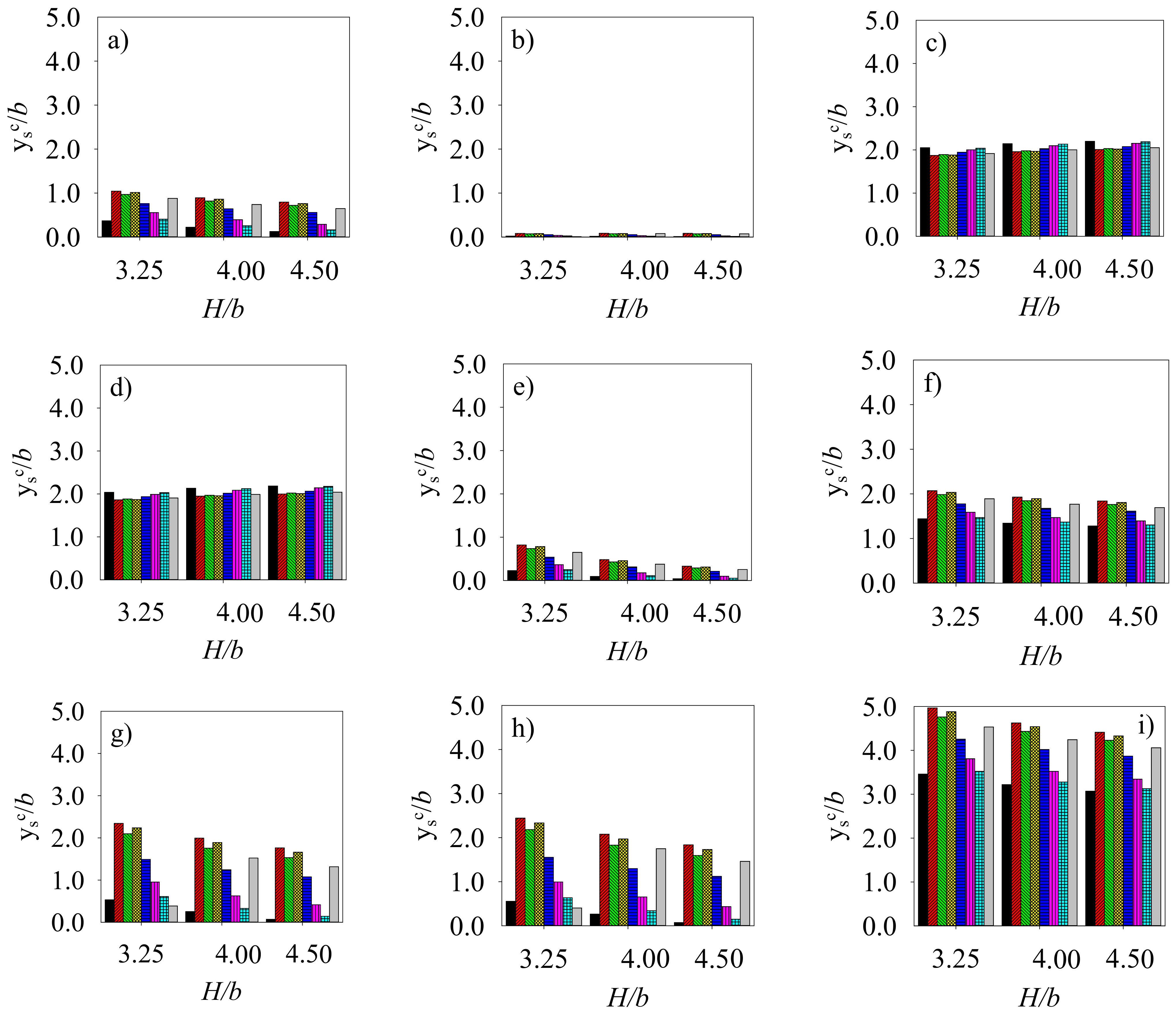
In this section, the first step is to calculate the equilibrium scour with a combination of scouring/critical velocity equations. This is done to show the variability in calculated scour depth with the various equations proposed. Figure 1a–j shows the calculated values of scour depth with different relationships for three flow depth to pier diameter ratios, i.e., H/b, equal to 3.25, 4, and 4.5. Although the scour depth predicted by most of the hybrid equations is not close to the experimental results, it can be seen in Figure 1 that only the YKHA equation (Figure 1e) shows significant changes in the scour depth with the flow depth; for other equations, the scour depth is not significantly affected by changes in flow depth. Additionally, among the scour depth estimation equations, YJAF and YJAI equations show slight changes with different critical velocity equations. However, both the YGAO and YSGAO equations (Figure 1g,h) have the most variations with the different critical velocity equations used.

To accurately investigate how much each equation is affected by the critical velocity parameter, the sensitivity of each of the 10 critical velocity scouring equations is analyzed using the normalized sensitivity coefficient (Figure 2).

As can be seen in Figure 2, the YJAF, YJAI (multiplied by −1 to better show the negative values of Sc in the logarithmic scale), YMAS, YMEL, and YFDOT methods have the lowest critical flow velocity sensitivity among the equations studied.

The values of the four statistical parameters for the 80 hybrid relationships are available in

Table 4. Summary of statistical parameters used to compare the selected equations *.

	Model	VRAD	VSHI-a	VSHI-b	VVAN	VHAO	VHAN	VARN	VZHA
SSE
	YHAN	0.102	0.054	0.057	0.053	0.065	0.079	0.085	0.062
	YBRE	0.091	0.087	0.088	0.087	0.089	0.090	0.091	0.088
	YJAF	0.013	0.016	0.016	0.017	0.016	0.015	0.014	0.016
	YJAI	0.013	0.017	0.016	0.017	0.016	0.015	0.014	0.016
	YKHA	0.093	0.077	0.078	0.076	0.081	0.087	0.089	0.080
	YMAS	0.036	0.017	0.018	0.016	0.021	0.027	0.029	0.020
	YGAO	0.116	0.032	0.035	0.029	0.047	0.074	0.086	0.043
	YSGAO	0.119	0.021	0.025	0.017	0.038	0.070	0.083	0.034
	YMEL	0.017	0.065	0.057	0.068	0.040	0.023	0.019	0.046
	YFDOT	0.079	0.053	0.054	0.052	0.057	0.064	0.068	0.056
U
	YHAN	1.022	0.845	0.859	0.838	0.895	0.952	0.974	0.881
	YBRE	0.999	0.985	0.986	0.984	0.990	0.996	0.998	0.989
	YJAF	0.349	0.470	0.462	0.473	0.441	0.404	0.388	0.449
	YJAI	0.356	0.474	0.466	0.478	0.446	0.410	0.394	0.454
	YKHA	1.001	0.941	0.948	0.939	0.962	0.982	0.990	0.956
	YMAS	0.732	0.506	0.532	0.492	0.590	0.663	0.687	0.569
	YGAO	1.067	0.529	0.602	0.487	0.750	0.915	0.968	0.696
	YSGAO	1.067	0.516	0.592	0.473	0.744	0.913	0.967	0.689
	YMEL	0.338	0.886	0.848	0.904	0.751	0.588	0.517	0.789
	YFDOT	0.951	0.840	0.845	0.838	0.861	0.895	0.910	0.855
NNSE
	YHAN	0.145	0.705	0.644	0.675	0.475	0.275	0.218	0.554
	YBRE	0.164	0.185	0.183	0.186	0.176	0.168	0.166	0.179
	YJAF	0.071	0.100	0.098	0.102	0.091	0.082	0.079	0.094
	YJAI	0.072	0.102	0.099	0.104	0.093	0.083	0.080	0.095
	YKHA	0.167	0.314	0.291	0.316	0.248	0.200	0.184	0.268
	YMAS	0.424	0.106	0.117	0.098	0.154	0.238	0.277	0.140
	YGAO	0.101	0.127	0.180	0.103	0.465	0.391	0.229	0.349
	YSGAO	0.101	0.121	0.172	0.099	0.456	0.402	0.232	0.335
	YMEL	0.035	0.011	0.012	0.010	0.015	0.021	0.025	0.013
	YFDOT	0.285	0.605	0.596	0.596	0.557	0.451	0.391	0.582
NRMSE
	YHAN	2.042	1.493	1.529	1.468	1.627	1.796	1.863	1.592
	YBRE	1.934	1.890	1.895	1.887	1.907	1.924	1.930	1.903
	YJAF	0.735	0.820	0.814	0.827	0.799	0.773	0.766	0.803
	YJAI	0.738	0.824	0.818	0.831	0.803	0.777	0.769	0.807
	YKHA	1.954	1.779	1.795	1.769	1.823	1.890	1.908	1.807
	YMAS	1.207	0.831	0.856	0.802	0.928	1.050	1.092	0.906
	YGAO	2.184	1.149	1.204	1.090	1.393	1.747	1.876	1.334
	YSGAO	2.206	0.929	1.004	0.846	1.250	1.693	1.847	1.178
	YMEL	0.837	1.638	1.528	1.675	1.277	0.981	0.880	1.379
	YFDOT	1.803	1.469	1.483	1.460	1.526	1.621	1.664	1.510

* Underlined data indicate the lowest or highest values in each series.

. In addition to the three experimental runs carried out in the present study, a set of 14 experiments reported by [56] are used in the statistical analysis. As it can be seen, based on the SSE factor, the combined equations YJAF-VRAD, YJAI-VRAD, YJAF-VARN, and YJAI-VARN with SSE values of 0.013, 0.013, 0.014, and 0.014, respectively, have the highest accuracy in estimating scour depth in the range of flow conditions, sediment properties, and pier and channel geometry tested in the present study and those of reported by [56]. In addition, based on the U factor, the combined equations YMEL-VRAD, YJAF-VRAD, YJAI-VRAD, and YJAF-VARN with higher values of 0.338, 0.349, 0.356, and 0.388, respectively, show higher accuracy. If the NNSE factor is considered, the combined equations YFDOT-VSHI-a, YHAN-VSHI-b, YHAN-VVAN, and YHAN-VSHI-a with NNSE values of 0.605, 0.644, 0.675, and 0.705, respectively, give the best results. According to NRMSE statistical index, YJAF-VRAD, YJAI-VRAD, YJAF-VARN, and YJAI-VARN equations have higher accuracy with values of 0.735, 0.738, 0.766, and 0.769, respectively. These equations are actually in the category of the 5% most accurate results.

The best-performing models according to respective statistical indicators are listed in

Table 5. Top hybrid models according to the statistical indicators.

Statistical Indicators	Hybrid Model
SSE	YJAF-VRAD (0.013)	YJAI-VRAD (0.013)	YJAF-VARN (0.014)	YJAI-VARN (0.014)
U	YMEL-VRAD (0.338)	YJAF-VRAD (0.349)	YJAI-VRAD (0.356)	YJAF-VARN (0.388)
NNSE	YHAN-VVAN (0.675)	YHAN-VSHI-a (0.705)	YHAN-VSHI-b (0.644)	YFDOT-VSHI-a (0.605)
NRMSE	YJAF-VRAD (0.735)	YJAI-VRAD (0.738)	YJAF-VARN (0.766)	YJAI-VARN (0.769)

. Accordingly, YJAF-VRAD, YJAI-VRAD, and YJAF-VARN, are the best performing models in three cases out of four. In addition, the YJAI-VARN model ranked next best with two occurrences out of four possible cases. Overall, the hybrid models YJAF-VRAD, YJAI-VRAD, and YJAF-VARN can be suggested as the best models considering the statistical indicators studied. The reduced error of these models can be partially attributed to the reduced sensitivity from the sediment critical velocity parameter previously discussed, which makes these models less dependent on the errors in flow intensity estimate.

The selected hybrid equations are compared with field data to determine which of the equations perform best and can be recommended for practical use for bridge design. A total of 57 field data related to cylindrical bridge pier scour were collected from the literature [47,48]. While there are various datasets reported in the literature dealing with bridge pier scouring, these 57 data points were selected considering the experimental conditions of the present study. For example, only the data of cylindrical bridge piers were included in the analysis.

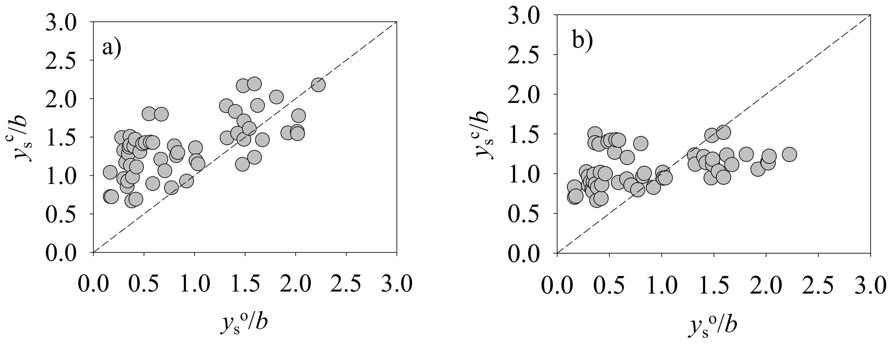
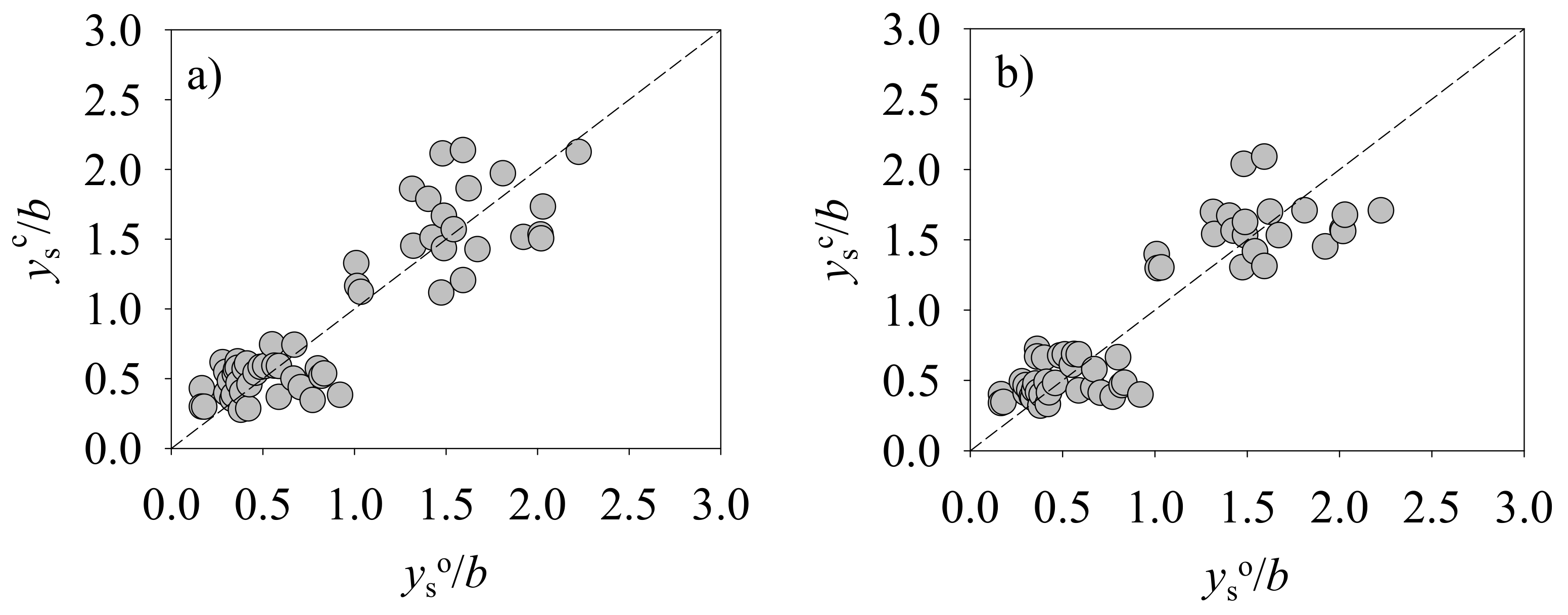
Variations of the calculated against measured scour depths are depicted in Figure 3a–c. In each graph, the closer the data points are to the perfect agreement line, the more accurate the corresponding equation. Figure 3 shows that the hybrid equations YJAF-VRAD and YJAF-VARN give almost similar conservative results while slightly overestimating the scour depth, and YJAI-VRAD hybrid equation is generally in better agreement with the observed data. It should be noted that laboratory-based formulas are usually conservative when applied to in-field case. The reason behind this could be the fact that the equilibrium scour depth is never attained under a single flood hydrograph, as discussed in previous studies [57,58].

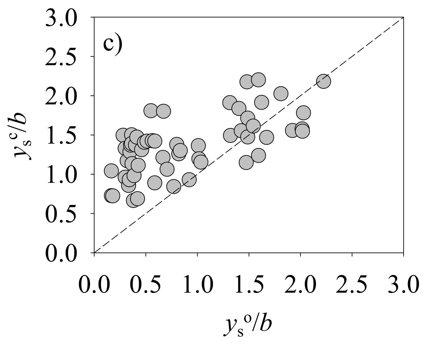
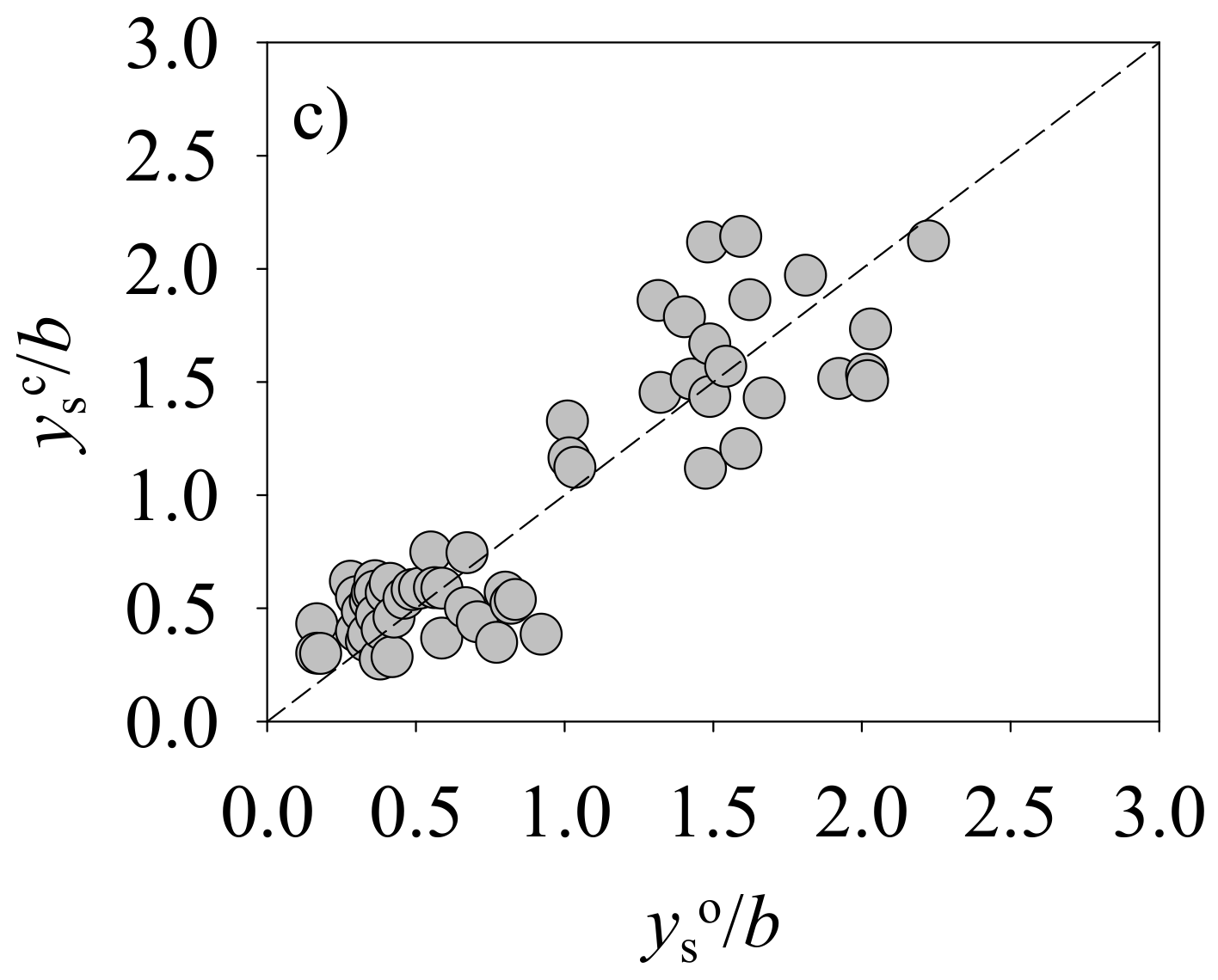
As shown in Figure 3a–c, most data in the range of y_s^o/b < 1 are above the perfect agreement line, which suggests that these equations provide a conservative estimate of scour depth for bridge pier design. An attempt was made to find a correction factor that can be applied in the three equations mentioned above for better agreement with the observed data. In this case, 80% of the field data were selected randomly as test data and the remaining 20% were used for validation. The correction coefficients obtained for the three selected hybrid equations including YJAF-VRAD, YJAI-VRAD, and YJAF-VARN are 0.41, 0.48, and 0.42, respectively, if y_s/b < 1 and 0.98, 1.38, 0.97, if y_s/b > 1. Figure 4a–c show that the data points get closer to the perfect agreement line after applying the correction factors, indicating an increase in the accuracy of the equations in predicting the scour depth around the pier. A good agreement can be observed between the predicted and measured scour depths for all of the top hybrid models using the mentioned correction factors. All three hybrid equations could be used by design engineers for a safer design of bridge piers against scouring whereas the YJAI equations give more precise results as it has the lowest sensitivity to the critical velocity variations among the scour depth prediction equations, as shown in Figure 2. It should be mentioned that using a correction factor to increase the accuracy of a bridge pier scour equation was suggested in a previous study [59].

4. Conclusions

Numerous experimental relationships exist in literature to predict the maximum scour depth around bridge piers. Given the variety of conditions tested in literature and observed in the field, the depth of scouring predicted in one method may be several times lower or higher than that predicted in the other method. The design engineer will be faced with a wide range of approaches and the choice of each of these methods will have its issues and limitations. An equation or combination of equations that severely underestimate the scour depth could severely damage bridge damage or lead to failure. Conversely, by overpredicting scouring depths, the construction costs could unnecessarily increase. In many of the proposed equations, the critical velocity or its dimensionless form, i.e., flow intensity, plays a critical role. In the present study, 10 of the most used equations for scour depth prediction around cylindrical bridge piers in cohesionless beds under clear water scour conditions, are combined with 8 different sediment critical velocity equations. A total of 80 combined relationships were compared using experimental data. The sensitivity of scouring relationships to the critical velocity was investigated and it was found that YJAI, YJAF, YMAS, and YMEL relationships have the lowest sensitivity to the critical flow velocity among the equations studied. Hence, an error in the critical flow velocity as the input variable in these relationships may be decreased in the output results.

The results of the hybrid models were also compared with the experimental data and the three best performing hybrid models were identified based on the highest statistical agreement with the observed data. The statistical methods included tail factor (U), normalized Nash–Sutcliffe efficiency coefficient (NNSE), normalized root-mean-square error (NRMSE), and the sum of squared error (SSE). It was found that while the YJAF-VRAD and YJAF-VARN models overestimated field scour depths, the results of the YJAI-VRAD hybrid model were in good agreement with the measured data. To decrease the difference between the predicted and measured values in the selected hybrid models, correction factors were introduced using regression analysis and were applied in the equations. Using the correction factors, a good agreement was observed between the predicted and measured scour depths for the three selected hybrid models.

References

- Wardhana, K.; Hadipriono, F.C. Analysis of Recent Bridge Failures in the United States. J. Perform. Constr. Facil. 2003, 17, 144–150. [Google Scholar] [CrossRef] [Green Version]
- Maddison, B. Scour failure of bridges. Proc. Inst. Civ. Eng. Forensic Eng. 2012, 165, 39–52. [Google Scholar] [CrossRef]
- Link, O.; García, M.; Pizarro, A.; Alcayaga, H.; Palma, S. Local Scour and Sediment Deposition at Bridge Piers during Floods. J. Hydraul. Eng. 2020, 146, 04020003. [Google Scholar] [CrossRef]
- Carnacina, I.; Pagliara, S.; Leonardi, N. Bridge pier scour under pressure flow conditions. River Res. Appl. 2019, 35, 844–854. [Google Scholar] [CrossRef]
- Boothroyd, R.J.; Williams, R.D.; Hoey, T.B.; Tolentino, P.L.; Yang, X. National-scale assessment of decadal river migration at critical bridge infrastructure in the Philippines. Sci. Total Environ. 2021, 768, 144460. [Google Scholar] [CrossRef]
- Keshavarzi, A.; Hamidifar, H.; Khajenoori, L. Mean Flow Structure and Local Scour around Single and Two Columns Bridge Piers. Irrig. Sci. Eng. 2019, 42, 75–90. [Google Scholar] [CrossRef]
- Keshavarzi, A.; Melville, B.W.; Ball, J. Three-dimensional analysis of coherent turbulent flow structure around a single circular bridge pier. Environ. Fluid Mech. 2014, 14, 821–847. [Google Scholar] [CrossRef]
- Keshavarzi, A.; Shrestha, C.K.; Zahedani, M.R.; Ball, J.; Khabbaz, H. Experimental study of flow structure around two in-line bridge piers. Proc. Inst. Civ. Eng. Water Manag. 2018, 171, 311–327. [Google Scholar] [CrossRef]
- Carnacina, I.; Lescova, A.; Pagliara, S. A Methodology to Measure Flow Fields at Bridge Piers in the Presence of Large Wood Debris Accumulation Using Acoustic Doppler Velocimeters. In Lecture Notes in Civil Engineering; Springer: Berlin/Heidelberg, Germany, 2020; Volume 39, pp. 17–25. [Google Scholar]
- Carnacina, I.; Leonardi, N.; Pagliara, S. Characteristics of Flow Structure around Cylindrical Bridge Piers in Pressure-Flow Conditions. Water 2019, 11, 2240. [Google Scholar] [CrossRef] [Green Version]
- Behrouzi, Z.; Hamidifar, H.; Zomorodian, M.A. Numerical simulation of flow velocity around single and twin bridge piers with different arrangements using the Fluent model. Amirkabir J. Civ. Eng. 2021, 53, 15. [Google Scholar] [CrossRef]
- Kayatürk, Ş.Y. Scour and Scour Protection at Bridge Abutments; Middle East Technical University: Ankara, Turkey, 2005. [Google Scholar]
- Kellermann, P.; Schönberger, C.; Thieken, A.H. Large-scale application of the flood damage model RAilway Infrastructure Loss (RAIL). Hazards Earth Syst. Sci. 2016, 16, 2357–2371. [Google Scholar] [CrossRef] [Green Version]
- MRUDI. Ministry of Roads & Urban Development Islamic Republic of Iran. Available online: https://www.mrud.ir/news-view/ArticleId/18024 (accessed on 24 November 2020).
- Macky, G.H. Survey of Roading Expenditure Due to Scour; Department of Scientific and Industrial Research, Hydrology Centre: Christchurch, New Zealand, 1990. [Google Scholar]
- Armitage, N.; Cunninghame, M.; Kabir, A.; Abban, B. Local Scour in Rivers. The Extent of the Problem in South Africa, The State of the Art of Numerical Modelling; University of Cape Town: Cape Town, South Africa, 2007. [Google Scholar]
- Nemry, F.; Demirel, H. Impacts of Climate Change on Transport: A Focus on Road and Rail Transport Infrastructures; Publications Office of the European Union, EU Science Hub: Luxembourg, 2012. [Google Scholar]
- Melville, B.W. Pier and Abutment Scour: Integrated Approach. J. Hydraul. Eng. 1997, 123, 125–136. [Google Scholar] [CrossRef]
- Parola, J.; Jones, J.S. Sizing riprap to protect bridge piers from scour. Transp. Res. Rec. 1991, 1290, 276–280. [Google Scholar]
- Johnson, P.A. Comparison of Pier-Scour Equations Using Field Data. J. Hydraul. Eng. 1995, 121, 626–629. [Google Scholar] [CrossRef]
- Etemad-Shahidi, A.; Bonakdar, L.; Jeng, D.-S. Estimation of scour depth around circular piers: Applications of model tree. J. Hydroinform. 2015, 17, 226–238. [Google Scholar] [CrossRef] [Green Version]
- Ebtehaj, I.; Sattar, A.M.A.; Bonakdari, H.; Zaji, A.H. Prediction of scour depth around bridge piers using self-adaptive extreme learning machine. J. Hydroinform. 2017, 19, 207–224. [Google Scholar] [CrossRef]
- Sharafati, A.; Tafarojnoruz, A.; Yaseen, Z.M. New stochastic modeling strategy on the prediction enhancement of pier scour depth in cohesive bed materials. J. Hydroinform. 2020, 22, 457–472. [Google Scholar] [CrossRef]
- Mohamed, T.A.; Pillai, S.; Noor, M.J.M.M.; Ghazali, A.H.; Huat, B.K.; Yusuf, B. Validation of Some Bridge Pier Scour Formulae and Models Using Field Data. J. King Saud Univ. Eng. Sci. 2006, 19, 31–40. [Google Scholar] [CrossRef]
- Gazi, A.H.; Afzal, M.S. A new mathematical model to calculate the equilibrium scour depth around a pier. Acta Geophys. 2020, 68, 181–187. [Google Scholar] [CrossRef]
- Sheykholeslami, M.; Shafaee-Bajestan, M.; Kashefi Poor, M. Estimation of Scour Depth at Bridge Piers by Using FASTER Model. Irrig. Water Eng. 2010, 1, 57–68. [Google Scholar]
- Laursen, E.M.; Toch, A. Scour around Bridge Piers and Abutments, HR-30 and Iowa Highway Research Board Bulletin No. 4; Iowa Highway Research Board: Ames, IA, USA, 1956; Volume 4. [Google Scholar]
- Koopaei, K.B.; Valentine, E.M. Bridge Pier Scour in Self Formed Laboratory Channels; Technical Report; University of Glasgow: Glasgow, UK, 2003. [Google Scholar]
- Pandey, M.; Zakwan, M.; Sharma, P.K.; Ahmad, Z. Multiple linear regression and genetic algorithm approaches to predict temporal scour depth near circular pier in non-cohesive sediment. ISH J. Hydraul. Eng. 2020, 26, 96–103. [Google Scholar] [CrossRef]
- Gaudio, R.; Grimaldi, C.; Tafarojnoruz, A.; Calomino, F. Comparison of formulae for the prediction of scour depth at piers. In Proceedings of the First European IAHR Congress, Edinburgh, UK, 4–6 May 2010; Heriot-Watt University: Edinburgh, UK; pp. 4–6. [Google Scholar]
- Gaudio, R.; Tafarojnoruz, A.; De Bartolo, S. Sensitivity analysis of bridge pier scour depth predictive formulae. J. Hydroinform. 2013, 15, 939–951. [Google Scholar] [CrossRef]
- Akhlaghi, E.; Babarsad, M.S.; Derikvand, E.; Abedini, M. Assessment the Effects of Different Parameters to Rate Scour around Single Piers and Pile Groups: A Review. Arch. Comput. Methods Eng. 2020, 27, 183–197. [Google Scholar] [CrossRef]
- Melville, B.W. The Physics of Local Scour at Bridge Piers. In Proceedings of the 4th International Conference on Scour and Erosion, Tokyo, Japan, 5–7 November 2008; The Japanese Geotechnical Society: Tokyo, Japan, 2008; pp. 28–40. [Google Scholar]
- Hancu, S. Sur Ie calcul des affouillements locaux dams la zone des piles de ponts. In Proceedings of the 14th IAHR Congress, Paris, France, 29 August–3 September 1971; IAHR: Paris, France, 1971; pp. 299–313. [Google Scholar]
- Breusers, H.N.C.; Nicollet, G.; Shen, H.W. Erosion locale autour des piles cylindriques. J. Hydraul. Res. 1977, 15, 211–252. [Google Scholar] [CrossRef]
- Jain, S.; Fischer, E. Scour around Circular Bridge Piers at High Froude Numbers; Final Report; US Department of Transportation, Federal Highway Administration: Washington, DC, USA, 1979.
- Jain, S.C. Maximum clear-water scour around circular piers. J. Hydraul. Div. 1981, 107, 611–626. [Google Scholar] [CrossRef]
- Khalfin, I.S. Local scour around ice-resistant structures caused by wave and current effect. In Proceedings of the Seventh International Conference on Port and Ocean Engineering under Arctic Conditions, Helsinki, Finland, 5–9 April 1983; pp. 992–1002. [Google Scholar]
- Melville, B.W.; Sutherland, A.J. Design Method for Local Scour at Bridge Piers. J. Hydraul. Eng. 1988, 114, 1210–1226. [Google Scholar] [CrossRef]
- Gao, D.; LilianPosada, G.; Nordin, C. Pier Scour Equations Used in China; Federal Highway Administration: Washington, DC, USA, 1993.
- Sheppard, D.M.; Renna, R. Bridge Scour Manual; Florida Department of Transportation: Tallahassee, FL, USA, 2005.
- Richardson, E.V.; Davis, S.R. Evaluating Scour at Bridges; No. FHWA-NHI-01-001; Federal Highway Administration: Washington, DC, USA, 2001.
- Henderson, F. Open Channel Flow; MacMillan Publishing Co.: New York, NY, USA, 1966. [Google Scholar]
- Van Rijn, L. Principles of Sediment Transport in Rivers, Estuaries and Coastal Seas; Aqua publications: Amsterdam, The Netherlands, 1993. [Google Scholar]
- Hager, W.H.; Oliveto, G. Shields’ Entrainment Criterion in Bridge Hydraulics. J. Hydraul. Eng. 2002, 128, 538–542. [Google Scholar] [CrossRef]
- Arneson, L.A.; Zevenbergen, L.W.; Lagasse, P.F.; Clopper, P.E. Evaluating Scour at Bridges; Report No. FHWA-HIF-12-003; Federal Highway Administration: Washington, DC, USA, 2012.
- Qadar, A. The Vortex Scour Mechanism at Bridge Piers. Proc. Inst. Civ. Eng. 1981, 71, 739–757. [Google Scholar] [CrossRef]
- Van Wilson, K. Scour at Selected Bridge Sites in Mississippi; US Department of the Interior, US Geological Survey: Reston, VA, USA, 1995.
- Gao, D.; Xu, G. Research on Local Scour Mechanism of Piers and Revision of the Equations; Xian Highway Transport University: Xian, China, 1989. [Google Scholar]
- Hao, L.; Gao, D. Hydraulics on Bridge Engineering; People’s Traffic Press: Beijing, China, 1991. [Google Scholar]
- Melville, B.W.; Chiew, Y.M. Time Scale for Local Scour at Bridge Piers. J. Hydraul. Eng. 1999, 125, 59–65. [Google Scholar] [CrossRef]
- Akhtaruzzaman Sarker, M. Flow measurement around scoured bridge piers using Acoustic-Doppler Velocimeter (ADV). Flow Meas. Instrum. 1998, 9, 217–227. [Google Scholar] [CrossRef]
- Breusers, H.; Raudkivi, A. Scouring, Hydraulic Structures Design Manual; IAHR: Rotterdam, The Netherlands, 1990; Volume 143. [Google Scholar]
- Farzadkhoo, M.; Keshavarzi, A.; Hamidifar, H.; James, B. Flow and longitudinal dispersion in channel with partly rigid floodplain vegetation. Proc. Inst. Civ. Eng. Water Manag. 2019, 172. [Google Scholar] [CrossRef]
- Keshavarzi, A.; Farzadkhoo, M.; Hamidifar, H. Longitudinal dispersion coefficient in compound open channel with rigid vegetation on flood plain. E3S Web Conf. 2018, 40, 02058. [Google Scholar] [CrossRef]
- Raeisi, N.; Ghomeshi, M. Effect of model scale in bridge piers scour experiments. Water Soil Sci. 2015, 25, 227–240. [Google Scholar]
- Tubaldi, E.; Macorini, L.; Izzuddin, B.A.; Manes, C.; Laio, F. A framework for probabilistic assessment of clear-water scour around bridge piers. Struct. Saf. 2017, 69, 11–22. [Google Scholar] [CrossRef] [Green Version]
- Pizarro, A.; Manfreda, S.; Tubaldi, E. The Science behind Scour at Bridge Foundations: A Review. Water 2020, 12, 374. [Google Scholar] [CrossRef] [Green Version]
- Johnson, P.A.; Clopper, P.E.; Zevenbergen, L.W.; Lagasse, P.F. Quantifying Uncertainty and Reliability in Bridge Scour Estimations. J. Hydraul. Eng. 2015, 141, 04015013. [Google Scholar] [CrossRef]
Figure 1.
Variations of the nondimensional predicted scour depths, ysc/b, against the nondimensional flow depths, H/b, for different scour prediction relationships: (a) YHAN, (b) YBRE, (c) YJAF, (d) YJAI, (e) YKHA, (f) YMAS, (g) YGAO, (h) YSGAO, (i) YMEL, (j) YFDOT.
Figure 2.
Sensitivity of the different scour prediction models to the critical velocity: (a) YHAN, (b) YBRE, (c) YJAF, (d) YJAI, (e) YKHA, (f) YMAS, (g) YGAO, (h) YSGAO, (i) YMEL, (j) YFDOT.
Figure 3.
Comparison of the nondimensional observed scour depth, yso/b, and the nondimensional calculated scour depth, ysc/b, for the selected hybrid models: (a) YJAF-VRAD, (b) YJAI-VRAD, and (c) YJAF-VARN (- - - - - - -) perfect agreement line.
Figure 4.
Comparison of the nondimensional observed scour depth, yso/b, and the nondimensional calculated scour depth, ysc/b, for the selected hybrid models after applying the correction factors: (a) YJAF-VRAD, (b) YJAI-VRAD, and (c) YJAF-VARN, (- - - - - - -) perfect agreement line.