
Testing the Sensitivity and Limitations of Frequently Used Aquatic Biota Indices in Temperate Mountain Streams and Plain Streams of China


Abstract
:1. Introduction
2. Methods
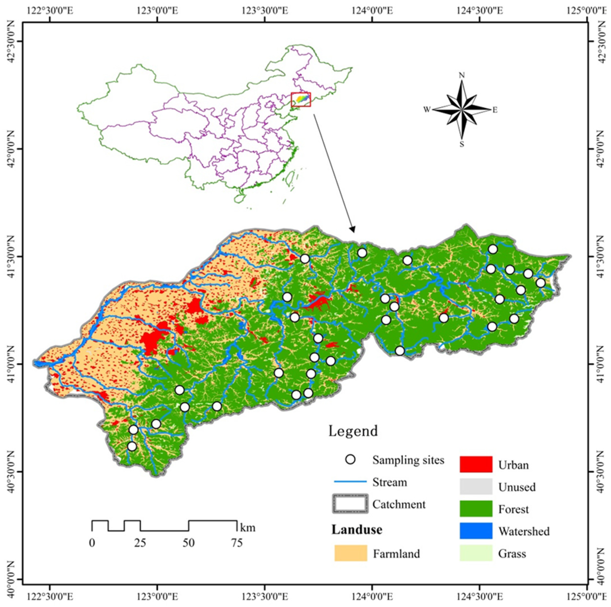
2.1. Study Area
2.2. Environmental Factors
2.3. Biological Assemblages
2.3.1. Macroinvertebrates
2.3.2. Fish
2.4. Land Use and Patterns at Various Scales
2.5. Data Analysis
2.5.1. Biological Indices Selected
2.5.2. Statistical Analysis
3. Results
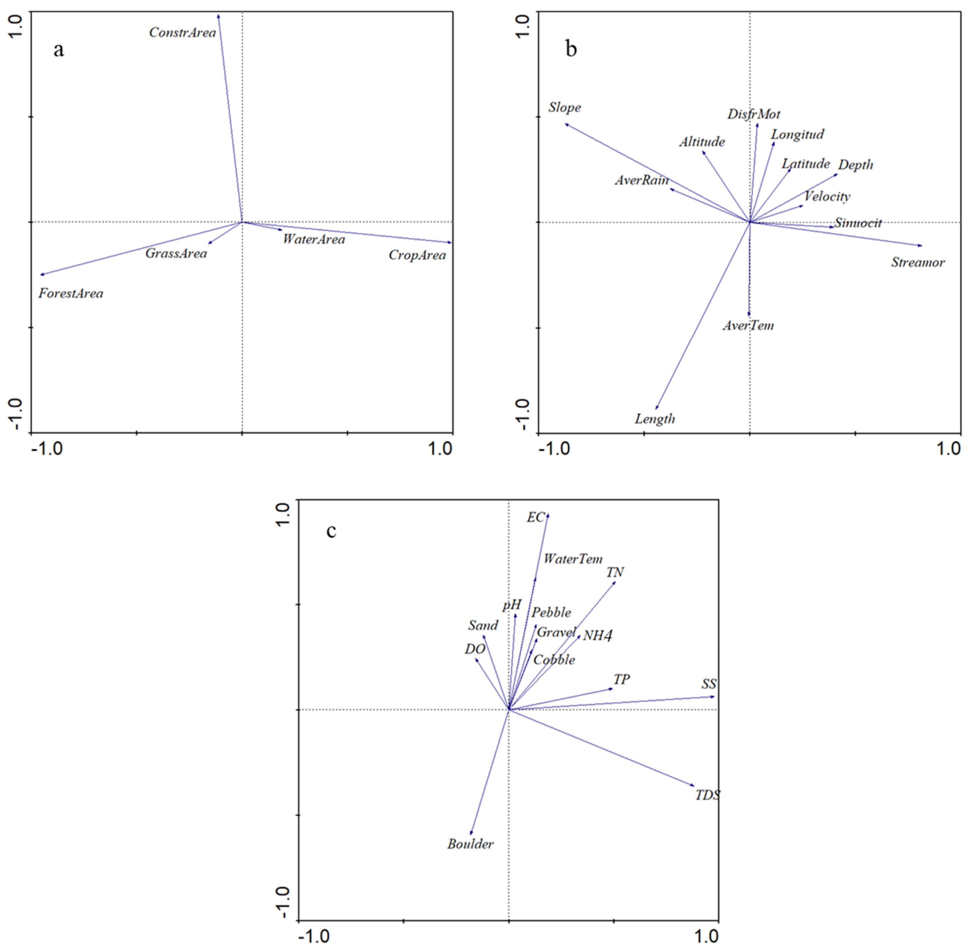
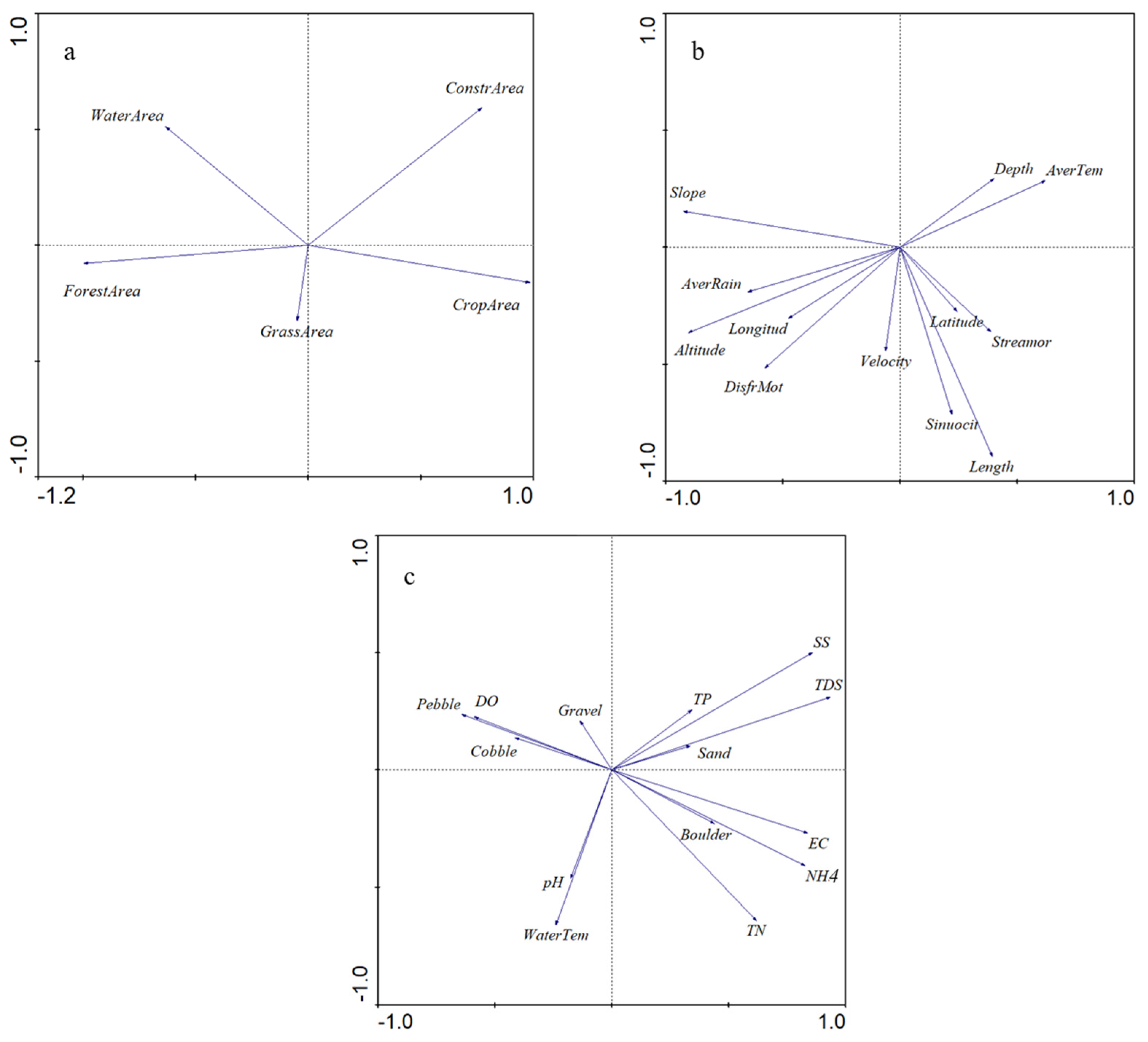
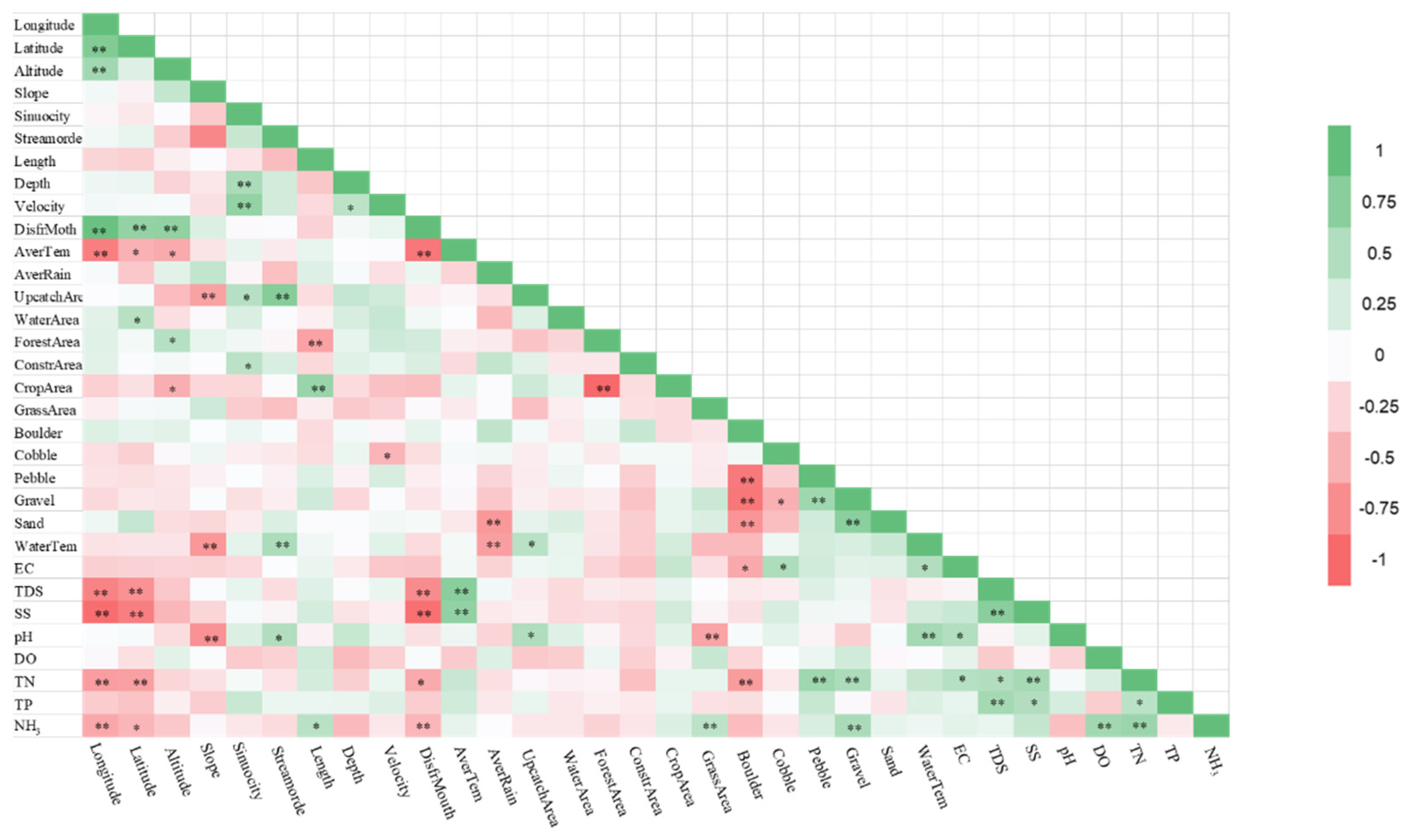
3.1. Comprehensive Environmental Gradient
3.2. Relationships between Biotic Indices and Environmental Variables
4. Discussion
Author Contributions
Funding
Institutional Review Board Statement
Informed Consent Statement
Data Availability Statement
Conflicts of Interest
References
- Meybeck, M. The global change of continental aquatic systems: Dominant impacts of human activities. Water Sci. Technol. 2004, 39, 73–83. [Google Scholar] [CrossRef]
- Furse, M.; Hering, D.; Moog, O.; Verdonschot, P.; Johnson, R.K.; Brabec, K.; Gritzalis, K.; Buffagni, A.; Pinto, P.; Friberg, N.; et al. The STAR project: Context, objectives and approaches. Hydrobiologia 2006, 566, 3–29. [Google Scholar] [CrossRef]
- Veldhuis, M.P.; Berg, M.P.; Loreau, M.; Olff, H. Ecological autocatalysis: A central principle in ecosystem organization? Ecol. Monogr. 2018, 88, 304–319. [Google Scholar] [CrossRef] [Green Version]
- Karr, J.R. Assessment of biotic integrity using fish communities. Fisheries 1981, 6, 21–27. [Google Scholar] [CrossRef]
- Capmourteres, V.; Rooney, N.; Anand, M. Assessing the causal relationships of ecological integrity: A re-evaluation of Karr’s iconic Index of Biotic Integrity. Ecosphere 2018, 9, e02168. [Google Scholar] [CrossRef] [Green Version]
- Birk, S.; Bonne, W.; Borja, A.; Brucet, S.; Courrat, A.; Poikane, S.; Solimini, A.; van de Bund, W.; Zampoukas, N.; Hering, D. Three hundred ways to assess Europe’s surface water: An almost complete overview of biological methods to implement the Water Framework Directive. Ecol. Indic. 2012, 18, 31–41. [Google Scholar] [CrossRef]
- Barbour, M.T.; Gerritsen, J.; Snyder, B.D.; Stribling, J.B. Rapid Bioassessment Protocols for Use in Streams and Wadeable Rivers: Periphyton, Benthic Macroinvertebrates and Fish, 2nd ed.; Environmental Protection Agency, Office of Water: Washington, DC, USA, 1999. [Google Scholar]
- Morin, S.; Gómez, N.; Tornés, E.; Licursi, M.; Rosebery, J. Benthic Diatom Monitoring and Assessment of Freshwater Environments: Standard Methods and Future Challenges; Romaní, A.M., Guasch, H., Balaguer, M.D., Eds.; Aquatic Biofilms: Ecology, Water Quality and Water Treatment; Caister Academic Press: Norfolk, UK, 2016. [Google Scholar]
- Stoll, S.; Kail, J.; Lorenz, A.W.; Sundermann, A.; Haase, P. The importance of the regional species pool, ecological species traits and local habitat conditions for the colonization of restored river reaches by fish. PLoS ONE 2014, 9, e84741. [Google Scholar]
- Santos, L.B.; Bruno, C.G.C.; Santos, J.C. Colonization by benthic macroinvertebrates in two artificial substrate types of a riparian forest. Acta Limnol. Bras. 2016, 28, e24. [Google Scholar] [CrossRef] [Green Version]
- Johnson, R.K.; Hering, D. Response of taxonomic groups in streams to gradients in resource and habitat characteristics. J. Appl. Ecol. 2009, 46, 175–186. [Google Scholar] [CrossRef]
- Johnson, R.K.; Ringler, N.H. The response of fish and macroinvertebrate assemblages to multiple stressors: A comparative analysis of aquatic communities in a perturbed watershed (Onondaga Lake, NY). Ecol. Indic. 2014, 41, 198–208. [Google Scholar] [CrossRef]
- Kolkwitz, R.; Marsson, M. Ökologie der tierischen Saprobien. Beiträge zur Lehre von der biologischen Gewässerbeurteilung. Int. Rev. Hydrobiol. 1909, 2, 126–152. [Google Scholar] [CrossRef] [Green Version]
- Karaouzas, I.; Smeti, E.; Kaloianni, E.; Skoulikidis, N.T. Ecological status monitoring and assessment in Greek rivers: Do macroinvertebrate and diatom indices indicate same responses to anthropogenic pressures. Ecol. Indic. 2019, 101, 126–132. [Google Scholar] [CrossRef]
- Li, T.; Huang, X.; Jiang, X.; Wang, X. Assessment of ecosystem health of the Yellow River with fish index of biotic integrity. Hydrobiologia 2015, 814, 31–43. [Google Scholar] [CrossRef]
- Arman, N.Z.; Salmiati, S.; Said, M.I.M.; Aris, A. Development of macroinvertebrate-based multimetric index and establishment of biocriteria for river health assessment in Malaysia. Ecol. Indic. 2019, 104, 449–458. [Google Scholar] [CrossRef]
- Hering, D.; Borja, A.; Carstensen, J.; Carvalho, L.; Elliott, M.; Feld, C.K.; Heiskanen, A.S.; Johnson, R.K.; Moe, J.; Pont, D.; et al. The European Water Framework Directive at the age of 10: A critical review of the achievements with recommendations for the future. Sci. Total Environ. 2010, 408, 4007–4019. [Google Scholar] [CrossRef] [Green Version]
- Johnson, R.K.; Heing, D.; Furse, M.T.; Clarke, R.T. Detection of ecological change using multiple organism groups: Metrics and uncertainty. Hydrobiologia 2006, 566, 115–137. [Google Scholar] [CrossRef]
- Abbasi, T.; Abbasi, S.A. Water quality indices based on bioassessment: The biotic indices. J. Water Health 2011, 9, 330–348. [Google Scholar] [CrossRef] [Green Version]
- Zhang, Y.; Wang, X.N.; Ding, H.Y.; Dai, Y.; Ding, S.; Gao, X. Threshold responses in the taxonomic and functional structure of fish assemblages to land use and water quality: A case study from the Taizi River. Water 2019, 11, 661. [Google Scholar] [CrossRef] [Green Version]
- Strahler, A.N. Hypsometric (area-altitude) analysis of erosional topology. Geol. Soc. Am. Bull. 1952, 63, 1117–1142. [Google Scholar] [CrossRef]
- State Environmental Protection Administration (SEPA), China. Water and Wastewater Monitoring and Analysis Methods, 4th ed.; Chinese Environmental Science Press: Beijing, China, 2002; ISBN 9787801634009. [Google Scholar]
- Li, L.; Zheng, B.; Liu, L. Biomonitoring and bioindicators used for river ecosystems: Definitions, approaches and trends. Procedia Environ. Sci. 2010, 2, 1510–1524. [Google Scholar] [CrossRef] [Green Version]
- Gao, X.; Ding, H.Y.; Xia, R.; Wang, H.; Kou, Q.Q.; Ding, S. Developing a modified umbrella index for conservation of macroinvertebrate diversity in Taizi River basin, China. Water 2020, 12, 857. [Google Scholar] [CrossRef] [Green Version]
- Qiu, S.W.; Li, F.H. On the problem of geomorphological classification in China. Sci. Geogr. Sin. 1982, 2, 327–335. (In Chinese) [Google Scholar]
- Wang, Y.K.; Stevenson, R.J.; Sweets, P.R.; Di Franco, J. Developing and testing diatom indicators for wetlands in the Casco Bay watershed, Maine, USA. In Advances in Algal Biology: A Commemoration of the Work of Rex Lowe; Stevenson, R.J., Pan, Y., Kociolek, J.P., Kingston, J.C., Eds.; Springer: Dordrecht, The Netherland, 2006; pp. 191–206. [Google Scholar]
- Yin, X.W.; Qu, X.D.; Li, Q.N.; Liu, Y.; Zhang, Y.; Meng, W. Using periphyton assemblages to assess stream conditions of Taizi River basin, China. Acta Ecol. Sin. 2012, 32, 1677–1691. (In Chinese) [Google Scholar]
- Qu, X.D.; Liu, Z.G.; Zhang, Y. Discussion on the standardized method of reference sites for establishing the benthic-index of biotic integrity. Acta Ecol. Sin. 2012, 32, 4661–4672. (In Chinese) [Google Scholar]
- Song, Z.G.; Wang, W.; Jiang, Z.Q.; Yin, X.W.; Tan, S.R.; Zhang, Y.; Meng, W. An assessment of ecosystem health in Taizi River basin using F-IBI. J. Dalian Ocean. Univ. 2010, 25, 480–487. (In Chinese) [Google Scholar]
- Legendre, P.; Legendre, L. Numerical Ecology, 3rd ed.; Elsevier Science: Amsterdam, The Netherland, 2012; ISBN 9780444538680. [Google Scholar]
- Lv, Y.; Sun, F.; Wang, J.; Zeng, Y.; Holmberg, M.; Böttcher, K.; Vanhala, P.; Fu, B. Managing landscape heterogeneity in different socio-ecological contexts: Contrasting cases from central Loess Plateau of China and southern Finland. Landsc. Ecol. 2015, 30, 463–475. [Google Scholar]
- Wang, X.; Tan, X. Macroinvertebrate community in relation to water quality and riparian land use in a substropical mountain stream, China. Environ. Sci. Pollut. Res. 2017, 24, 14682–14689. [Google Scholar] [CrossRef] [PubMed]
- Zhang, Y.; Zhao, R.; Kong, W.; Geng, S.; Bentsen, C.N.; Qu, X. Relationships between macroinvertebrate communities and land use types within different riparian widths in three headwater streams of Taizi River, China. J. Freshw. Ecol. 2013, 28, 307–328. [Google Scholar] [CrossRef]
- Zhang, Y.; Zhao, Q.; Ding, S. The response of stream fish to the gradient of conductivity: A case study from the Taizi River, China. Aquat. Ecosyst. Health Manag. 2019, 22, 171–182. [Google Scholar] [CrossRef]
- Yan, Y.Z.; Zhan, Y.J.; Chu, L.; Chen, Y.F.; Wu, C.H. Effects of stream size and spatial position on stream-dwelling fish assemblages. Acta Hydrobiol. Sin. 2010, 34, 1022–1030. (In Chinese) [Google Scholar] [CrossRef]
- Yu, X.D.; Luo, T.H.; Zhou, H.Z. Large-scale patterns in species diversity of fishes in the Yangtze River Basin. Biodivers. Sci. 2005, 13, 473–495. (In Chinese) [Google Scholar] [CrossRef]
- Girard, C.E.; Walters, A.W. Evaluating relationships between native fishes and habitat in streams affected by oil and natural gas development. Fish. Manag. Ecol. 2018, 25, 366–379. [Google Scholar] [CrossRef]
- Gerhard, P.; Moraes, R.; Molander, S. Stream fish communities and their associations to habitat variables in a rain forest reserve in southerstern Brazil. Environ. Biol. Fish. 2004, 71, 321–340. [Google Scholar] [CrossRef]
- Zhang, Y.; Ding, S.; Bentsen, C.N.; Ma, S.; Jia, X.; Meng, W. Differences in stream fish assemblages subjected to different levels of anthropogenic pressure in the Taizi River catchment, China. Ichthyol. Res. 2015, 62, 450–462. [Google Scholar] [CrossRef]
- Johnson, R.K.; Furse, M.T.; Hering, D.; Sandin, L. Ecological relationships between stream communities and spatial scale: Implications for designing catchment-level monitoring programs. Freshw. Biol. 2007, 52, 939–958. [Google Scholar] [CrossRef]
- Wilkinson, C.L.; Yeo, D.C.J.; Hui, T.H.; Fikri, A.H.; Ewers, R.M. Land-use change is associated with a significant loss of freshwater fish species and functional richness in Sabah, Malaysia. Biol. Conser. 2018, 222, 164–171. [Google Scholar] [CrossRef]
- Leitao, R.P.; Zuanon, J.Z.; Mouillot, D.; Leal, C.G.; Hughes, R.M.; Jaufmann, P.R.; Villeger, S.; Pompeu, P.S.; Kasper, D.; de Paula, F.R.; et al. Disentangling the pathways of land use impacts on the functional structure of fish assemblages in Amazon streams. Ecography 2018, 41, 219–232. [Google Scholar] [CrossRef]
- Flinders, C.A.; Horwitz, R.J.; Beltton, T. Relationship of fish and macroinvertebrate communities in the mid-Atlantic uplands: Implications for integrated assessment. Ecol. Indic. 2008, 8, 588–598. [Google Scholar] [CrossRef]
- Jonsson, N. Influence of water flow, water temperature and light on fish migration in rivers. Nord. J. Freshw. Res. 1991, 66, 20–35. [Google Scholar]
- Griffith, M.B.; Hill, B.H.; McCormick, F.H.; Kaufmann, P.R.; Herlihy, A.T.; Selle, A.R. Comparative application of indices of biotic integrity based on periphyton, macroinvertebrates, and fish to southern Rocky Mountain streams. Ecol. Indic. 2005, 5, 117–136. [Google Scholar] [CrossRef]
- Schäffer, M.; Hellmann, C.; Avlyush, S.; Borchardt, D. The key role of increased fine sediment loading in shaping macroinvertebrate communities along a multiple stressor gradient in a Eurasian steppe river (Kharaa River, Mongolia). Int. Rev. Hydrobiol. 2020, 105, 5–19. [Google Scholar] [CrossRef] [Green Version]
- Beisel, J.N.; Usseglio-Polatera, P.; Moreteau, J.C. The spatial heterogeneity of a river bottom: A key factor determining macroinvertebrate communities. Hydrobiologia 2000, 422–423, 163–171. [Google Scholar] [CrossRef]
- Huang, Q.; Gao, J.F.; Cai, Y.J.; Yin, H.B.; Gao, Y.N.; Zhao, J.H.; Liu, L.Z.; Huang, J.C. Development and application of benthic macroinvertebrate-based multimetric indices for the assessment of streams and rivers in theTaihu Basin, China. Ecol. Indic. 2014, 48, 649–659. [Google Scholar] [CrossRef]
- Yang, Z.; Zhu, D.; Zhu, Q.G.; Hu, L.; Wan, C.Y.; Zhao, N.; Liu, H.; Chen, X.J. Development of new fish-based indices of biotic integrity for estimating the effects of cascade reservoirs on fish assemblages in the upper Yangtze River, China. Ecol. Indic. 2020, 119, 106860. [Google Scholar] [CrossRef]
- You, Q.; Yang, W.; Jian, M.; Hu, Q. A comparison of metric scoring and health status classification methods to evaluate benthic macroinvertebrate-based index of biotic integrity performance in Poyang Lake wetland. Sci. Total Environ. 2021, 761, 144112. [Google Scholar] [CrossRef] [PubMed]
- Freund, J.G.; Petty, J.T. Response of fish and macroinvertebrate bioassessment indices to water chemistry in a mined Appalachian watershed. Environ. Manag. 2007, 39, 707–720. [Google Scholar] [CrossRef] [PubMed]


| Variable | First Quartile | Median | Third Quartile | Mean | SD | Range |
|---|---|---|---|---|---|---|
| Watershed characteristics | ||||||
| Catchment area (km2) | 52.94 | 95.36 | 326.98 | 3243.67 | 597.32 | 17.26–3407.75 |
| Water area (m2) | 0 | 0 | 0.0043 | 0.0088 | 0.0173 | 0–0.05 |
| Forest area (m2) | 0.58 | 0.71 | 0.78 | 0.64 | 0.24 | 0–0.91 |
| Construction area (m2) | 0.0038 | 0.01023 | 0.05508 | 0.036 | 0.047 | 0–0.20 |
| Crop area (m2) | 0.188 | 0.234 | 0.377 | 0.0306 | 0.209 | 0.018–0.891 |
| Grass area (m2) | 0 | 0 | 0.015 | 0.011 | 0.019 | 0–0.069 |
| Water physicochemical conditions | ||||||
| pH | 8.0 | 8.3 | 8.5 | 8.2 | 0.4 | 7.0–8.8 |
| EC (μS/cm) | 189.5 | 281.0 | 424.5 | 313.2 | 195.4 | 89.0–1133.0 |
| TDS (mg/L) | 169.0 | 280.0 | 335.3 | 277.1 | 156.1 | 51.0–746.5 |
| DO (mg/L) | 6.0 | 6.9 | 7.8 | 7.1 | 1.7 | 3.9–13.5 |
| BOD5 (mg/L) | 2.7 | 4.0 | 5.3 | 5.3 | 4.9 | 1.9–28.7 |
| CODMn (mg/L) | 1.8 | 2.4 | 4.0 | 3.1 | 1.7 | 1.4–8.3 |
| TN (mg/L) | 1.5 | 2.1 | 3.2 | 3.1 | 3.0 | 0.8–17.0 |
| TP (mg/L) | 0.0 | 0.1 | 0.2 | 0.2 | 0.3 | 0.0–1.6 |
| NH4-N (mg/L) | 0.1 | 0.1 | 0.5 | 0.7 | 2.2 | 0.03–13.2 |
| SS (mg/L) | 23.75 | 69 | 119.25 | 108.49 | 152.11 | 11.5–884 |
| Cobble | 0.114 | 0.164 | 0.200 | 0.18 | 0.11 | 0–0.57 |
| Pebble | 0.196 | 0.289 | 0.368 | 0.28 | 0.12 | 0.04–0.52 |
| Gravel | 0.069 | 0.109 | 0.196 | 0.14 | 0.10 | 0.01–0.45 |
| Sand | 0.021 | 0.043 | 0.102 | 0.076 | 0.085 | 0.003–0.389 |
| Hydrological characteristics | ||||||
| Depth (cm) | 13.7 | 18.3 | 24.3 | 19.5 | 9.6 | 5.0–52.0 |
| Velocity (m/s) | 0.25 | 0.37 | 0.44 | 0.37 | 0.17 | 0.0–0.8 |
| Altitude (m) | 149.5 | 256 | 385 | 263.86 | 139.03 | 8–546 |
| Slope (%) | 3.66 | 7.05 | 13.48 | 9.13 | 7.37 | 0–29.92 |
| Sinuosity | 1.09 | 1.24 | 1.42 | 1.29 | 0.27 | 1–2.12 |
| Stream order | 1 | 2 | 3 | 1.97 | 0.81 | 1–3 |
| Length (m) | 4.90 | 7.16 | 17.36 | 11.75 | 9.84 | 0.72–35.1 |
| Distance from mouth | 292,352 | 34,535 | 455,650 | 346,843.2 | 105,337.4 | 130,574–504,743 |
| Average temperature (°C) | 4.92 | 5.83 | 7.15 | 5.86 | 1.89 | 3.22–9.01 |
| Average rainfall (mm) | 835.2 | 899.3 | 950.65 | 876.10 | 81.37 | 650.9–954.6 |
| Longitude | 123.48 | 123.75 | 124.44 | 123.85 | 0.62 | 122.68–124.79 |
| Latitude | 40.92 | 41.21 | 41.36 | 41.15 | 0.27 | 40.62–41.60 |
| Water temperature (°C) | 19.2 | 21.5 | 24.1 | 21.03 | 3.37 | 14–26.5 |
| Abbreviation | Index Parameter | Mountain and Hilly Rivers | Plain Rivers | ||||
|---|---|---|---|---|---|---|---|
| PCA Axis 1 (Catchment Scale) | PCA Axis 1 (Reach Scale) | PCA Axis 1 (Site Scale) | PCA Axis 1 (Catchment Scale) | PCA Axis 1 (Reach Scale) | PCA Axis 1 (Site Scale) | ||
| F1 | Number of fish species | 0.355 | 0.474 * | −0.163 | −0.197 | −0.41 | −0.464 |
| F2 | Diversity index | 0.242 | 0.533 ** | 0.192 | 0.192 | −0.232 | −0.088 |
| F3 | Percentage of Gobiaceae | 0.458 * | 0.302 | 0.242 | 0.017 | 0.207 | −0.066 |
| F4 | Percentage of Cyprinidae | 0.093 | 0.196 | −0.385 | 0.668 * | 0.813 ** | 0.904 ** |
| F5 | Percentage of Cobitidae | 0.09 | −0.31 | 0.07 | −0.381 | −0.625 * | −0.63 * |
| F5 | Percentage of Cobitidae | 0.121 | −0.352 | 0.116 | −0.371 | −0.642 * | −0.655 |
| F6 | Percentage of Leuciscinae | −0.283 | −0.279 | −0.315 | −0.515 | −0.557 | −0.654 * |
| F7 | Percentage of Gobiidae | 0.061 | −0.064 | 0.009 | −0.166 | 0.009 | 0.192 |
| F8 | Percentage of pelagic fish | −0.058 | 0.393 | 0.364 | 0.249 | −0.15 | 0.241 |
| F9 | Percentage of bottom-dwelling fish | 0.156 | −0.175 | 0.039 | −0.463 | −0.232 | −0.411 |
| F10 | Percentage of lower- and middle-class fish | −0.154 | −0.078 | −0.286 | 0.09 | 0.266 | 0.107 |
| F12 | Percentage of herbivorous fish | −0.285 | 0.435 * | −0.23 | −0.038 | 0.413 | 0.209 |
| F13 | Percentage of omnivorous fish | −0.043 | −0.069 | 0.031 | −0.223 | −0.526 | −0.326 |
| F14 | Percentage of benthic feeders | −0.102 | −0.263 | −0.049 | 0.559 | 0.316 | 0.363 |
| F15 | Percentage of tolerant fish | 0.235 | 0.243 | −0.013 | 0.336 | 0.632 * | 0.625 * |
| F16 | Percentage of sensitive fish | 0.026 | 0.613 ** | −0.32 | −0.49 | −0.566 | −0.698 * |
| F17 | Percentage of pelagic egg fish | −0.28 | −0.305 | −0.401 | 0.710 ** | 0.507 | 0.721 ** |
| F18 | Percentage of demersal egg fish | 0.177 | 0.351 | 0.153 | −0.065 | −0.369 | −0.077 |
| F19 | Percentage of viscid egg fish | −0.06 | 0.389 | 0.362 | −0.519 | −0.413 | −0.547 |
| F20 | Percentage of fish with special spawning methods | −0.125 | −0.525 * | −0.35 | 0.082 | 0.623 * | 0.405 |
| F21 | Individual number | 0.097 | 0.144 | −0.311 | −0.337 | −0.462 | −0.668 * |
| F22 | Percentage of cold-water fish | 0.275 | −0.272 | −0.062 | −0.506 | −0.640 * | −0.716 ** |
| F24 | Percentage of widely distributed species (frequency >50%) | −0.163 | −0.537 ** | −0.226 | −0.506 | −0.557 | −0.716 ** |
| M1 | Total taxa | −0.108 | 0.454 * | −0.530 * | −0.741 ** | −0.517 | −0.649 * |
| M2 | EPT | −0.215 | 0.531 * | −0.453 * | −0.607 * | −0.569 | −0.61 * |
| M3 | Ephemeroptera | −0.469 * | 0.595 ** | −0.453 * | −0.599 * | −0.589 * | −0.573 |
| M4 | Plecoptera | 0.106 | −0.149 | −0.354 | 0.199 | 0.458 | 0.395 |
| M5 | Trichoptera | 0.088 | 0.430 * | −0.273 | −0.544 | −0.505 | −0.612 * |
| M6 | Amphipoda + Mollusca | 0.226 | −0.162 | −0.23 | −0.446 | −0.204 | −0.126 |
| M7 | Pleccoptera % | −0.075 | −0.259 | −0.252 | 0.199 | 0.458 | 0.395 |
| M8 | Ephemeroptera % | −0.442 * | 0.171 | −0.037 | −0.233 | −0.337 | −0.168 |
| M9 | Trichoptera % | 0.016 | 0.167 | 0.351 | −0.472 | −0.222 | −0.373 |
| M10 | EPT % | −0.356 | 0.236 | 0.188 | −0.357 | −0.317 | −0.263 |
| M11 | Chironomidae % | 0.314 | −0.195 | −0.299 | 0.04 | −0.46 | −0.356 |
| M12 | Diptera % | 0.358 | −0.08 | −0.255 | −0.002 | −0.505 | −0.401 |
| M13 | Amphipoda + Mollusca % | 0.167 | −0.347 | 0.144 | −0.498 | −0.304 | −0.44 |
| M14 | Oligochaeta % | 0.06 | −0.316 | −0.022 | 0.642 * | 0.826 ** | 0.835 ** |
| M15 | Intolerant taxa | −0.231 | 0.393 | −0.571 ** | −0.538 | −0.521 | −0.461 |
| M16 | Relative abundance of species number of fouling-tolerant groups | 0.085 | −0.207 | 0.018 | 0.607 * | 0.598 * | 0.703 * |
| M17 | Relative abundance of the most dominant taxa | 0.4 | −0.179 | 0.017 | 0.453 | 0.354 | 0.334 |
| M18 | Filterer % | 0.02 | 0.024 | 0.318 | 0.579 * | 0.864 ** | 0.829 ** |
| M19 | Scraper % | −0.357 | 0.077 | −0.04 | −0.207 | −0.249 | −0.134 |
| M20 | Collector/Gatherer % | 0.324 | 0.068 | −0.123 | −0.557 | −0.904 ** | −0.863 ** |
| M21 | Predator % | −0.352 | −0.28 | −0.313 | −0.038 | 0.151 | 0.117 |
| M22 | Shredder % | 0.082 | −0.319 | −0.215 | −0.227 | 0.068 | −0.109 |
| M23 | Clinger % | −0.403 | 0.245 | 0.046 | −0.424 | −0.249 | −0.375 |
| M24 | Clinger taxa | −0.214 | 0.488 * | −0.381 | −0.556 | −0.504 | −0.512 |
| M25 | Shannon | −0.433 * | 0.311 | −0.124 | −0.525 | −0.462 | −0.465 |
| M26 | Margalef | −0.121 | 0.442 * | −0.338 | −0.663 * | −0.558 | −0.625 * |
| M27 | Evenness | −0.426 * | 0.13 | 0.179 | −0.401 | −0.448 | −0.405 |
| M28 | Simpson | −0.394 | 0.209 | −0.021 | −0.543 | −0.445 | −0.459 |
| M29 | B-IBI | −0.166 | 0.383 | −0.315 | −0.737 ** | −0.417 | −0.516 |
| M30 | BMWP | 0.095 | 0.069 | −0.555 ** | −0.571 | −0.386 | −0.45 |
| M31 | FBI | −0.205 | 0.063 | 0.174 | 0.561 | 0.774 ** | 0.821 ** |
| M32 | BI | 0.468 * | −0.284 | 0.012 | 0.762 ** | 0.785 ** | 0.876 ** |
Publisher’s Note: MDPI stays neutral with regard to jurisdictional claims in published maps and institutional affiliations. |
© 2021 by the authors. Licensee MDPI, Basel, Switzerland. This article is an open access article distributed under the terms and conditions of the Creative Commons Attribution (CC BY) license (https://creativecommons.org/licenses/by/4.0/).
Share and Cite
Zhang, N.; Shang, G.; Dai, Y.; Zhang, Y.; Ding, S.; Gao, X. Testing the Sensitivity and Limitations of Frequently Used Aquatic Biota Indices in Temperate Mountain Streams and Plain Streams of China. Water 2021, 13, 3318. https://0-doi-org.brum.beds.ac.uk/10.3390/w13233318
Zhang N, Shang G, Dai Y, Zhang Y, Ding S, Gao X. Testing the Sensitivity and Limitations of Frequently Used Aquatic Biota Indices in Temperate Mountain Streams and Plain Streams of China. Water. 2021; 13(23):3318. https://0-doi-org.brum.beds.ac.uk/10.3390/w13233318
Chicago/Turabian StyleZhang, Nan, Guangxia Shang, Yang Dai, Yuan Zhang, Sen Ding, and Xin Gao. 2021. "Testing the Sensitivity and Limitations of Frequently Used Aquatic Biota Indices in Temperate Mountain Streams and Plain Streams of China" Water 13, no. 23: 3318. https://0-doi-org.brum.beds.ac.uk/10.3390/w13233318