Article

Daily Samples Revealing Shift in Phytoplankton Community and Its Environmental Drivers during Summer in Qinhuangdao Coastal Area, China

1
Center for Marine Environmental Ecology, School of Environmental Science and Engineering, Tianjin University, Tianjin 300072, China
2
The Eighth Geological Brigade, Hebei Geological Prospecting Bureau, Qinhuangdao 066001, China
3
Marine Ecological Restoration and Smart Ocean Engineering Research Center of Hebei Province, Qinhuangdao 066001, China
4
School of Civil Engineering, Tianjin University, Tianjin 300072, China
*
Authors to whom correspondence should be addressed.
Submission received: 30 March 2022 / Revised: 14 May 2022 / Accepted: 17 May 2022 / Published: 18 May 2022
(This article belongs to the Special Issue Diversity and Dynamics of Microbial Communities in Marine Ecosystems)

Abstract

:
Rapid urbanization and economic development in coastal regions have significantly increased coastal nutrient pollution and remarkably changed the phytoplankton community and developed some species into bloom, resulting in large economic losses and serious threats to public health. Therefore, it is indispensable to reveal the shift in the phytoplankton community and phytoplankton abundance, and phytoplankton’s environmental drivers. However, previous studies could not present the details of the environmental drivers of phytoplankton due to samples being collected with low temporal resolution. Here, high-temporal-resolution (daily) samples were collected to investigate the influence of environmental factors on phytoplankton in Qinhuangdao for 44 days. Phytoplankton communities showed a rapid succession, with predominant genera changing in the order SkeletonemaChaetocerosSkeletonemaThalassiosira. Similarly, Thalassiosira pacifica, Skeletonema costatum, Chaetoceros tortissimus, and Chattonella marina were identified as the dominant species and were abundant in 0–1.27 × 10⁷ cells·L−1, 0–9.34 × 10⁶ cells·L−1, 0–6.49 × 10⁶ cells·L−1, and 0–3.64 × 10⁶ cells·L−1, respectively. Moreover, inflows facilitate the rapid succession of the phytoplankton community. Dissolved inorganic phosphorus (DIP) was found to remarkably influence the succession of phytoplankton communities and the bloom of the top three dominant species, i.e., Thalassiosira pacifica, Skeletonema costatum, and Chaetoceros tortissimus. Overall, our results provide high-temporal-resolution observations of phytoplankton community succession and reveal its environmental drivers. This contributes to our current understanding of the occurrence of algae blooms and supports the development of management strategies to control algae bloom in coastal waters.

1. Introduction

Phytoplankton influences ecosystem productivity and food web structures at all scales and is directly linked to the global biogeochemical cycling of major elements, such as nitrogen, phosphorus, silicon, and carbon [1,2,3]. However, rapid urbanization and economic development in the coastal regions have significantly changed the phytoplankton community and facilitated toxic and nontoxic species blooms [4], resulting in adverse impacts on human health, aquaculture, the tourism industry, and the entire economy of the coastal region [5]. It is estimated that algae blooms lead to a global medical burden of 30.3 M USD every year [6]. Therefore, it is indispensable to understand the ecology of phytoplankton in coastal waters to better manage the coastal environment.
Inflows have been demonstrated to substantially impact phytoplankton abundance, community and diversity [7,8,9]. Relatively abundant phytoplankton is always observed in coastal regions with continuous low flows, which supply enough nutrients for phytoplankton growth [7,10]. Dramatically enhanced inflows disrupt the stable environment, reducing water retention time [7], inputting more nutrients, and disturbing sediments to release more nutrients [11]. The changes in these environmental factors shift both the abundance and the community of phytoplankton. It is reported that dramatically increased inflows facilitate the diatoms being replaced by chlorophytes in Biscayne Bay, FL, USA [12]. Additionally, another microcosm experiment demonstrated that pulsed inflows resulted in lower phytoplankton biomass and higher diversity [10]. However, dramatically enhanced inflows always occur with rainfall or flood discharge events, which are quick and transient. Thus, high-frequency samples are required to observe the impact of increased inflows on phytoplankton.
Temporal observation is a powerful tool to reveal the environmental drivers of the shift in phytoplankton [13,14,15]. Monthly samples collected in Qinhuangdao, China demonstrated that the phytoplankton community was dominated by different environmental factors in different seasons. The phytoplankton community was influenced by salinity in summer, while it was restricted by temperature in Autumn [13]. Weekly samples collected in the estuary demonstrated that phytoplankton communities may be affected by freshwater discharge, which not only changed physical factors such as hydrodynamic force, turbidity, and salinity but also shifted the nutrient supply [14]. For example, salinity, nitrogen, and phosphorus availability drive the shift in dominant groups in St. Lucia Estuary [15]. Meanwhile, PO4 and NH4 were also found to positively related to the formation of algae bloom in urban Thessaloniki Bay, Greece [5]. However, phytoplankton community and abundance may quickly respond to the shift in environmental factors. Due to the low frequency of observations in these studies, it is hard to fully capture the shift in the phytoplankton community and abundance and to identify their ecological drivers.
Qinhuangdao is a famous seaside tourist city in north China, and located in the Bohai Sea, which has a relatively weak water exchange [16]. In addition, along the coastal area of Qinhuangdao, there are more than 17 rivers, which input nutrients into coastal waters. In the last decade, algae bloom events have frequently been observed and have had a significant influence on economic development. Generally, algae bloom starts in April and peaks in July in Qinhuangdao, China [13]. A large-scale brown tide occurred in the Qinhuangdao coastal area from June to August 2012, covering 3400 km2 and lasting for 73 days [17]. Recently, small-scale algae blooms have been also frequently observed in the Qinhuangdao coast (Hebei Provincial Department of Land and Resources Oceanic Administration, 2021). Therefore, Qinhuangdao provides a suitable region to reveal the ecology of phytoplankton blooms.
In this study, high-resolution time series samples (daily samples) were collected in summer, which was a high-incidence season for algae blooms, in the coastal region influenced by a small river in Qinhuangdao, China. The ultimate goals of this study were to evaluate the variability in phytoplankton structure and its relationship with environmental drivers. The results of this paper expand the knowledge of the succession of the phytoplankton community and phytoplankton bloom and benefit the development of management strategies to control algae blooms in coastal waters.

2. Materials and Methods

2.1. Study Area and Water Sampling

The Qinhuangdao coastal area is located in the coastal area of the Northwestern Bohai Sea, China. It is a famous summer resort area in China that is well-known for its beautiful beaches and pleasant climate. This area is characterized by a typical continental monsoon climate; dry and rainless springs; tepidity without intense heat in the summers; cool autumns; and dry winters.
The sampling site was located in Jinmeng Bay, Qinhuangdao, Hebei Province and was influenced by Qiandaoxi River (Figure 1). The depth of the sampling site was about 2 m and inshore water samples were collected daily at a fixed site from 10 July 2021 to 22 August 2021. Approximately 2.5 L of near-surface seawater (1 m depth) was collected at 3:00 p.m. every day, and all samples were immediately stored in a cooler with ice packs (~4 °C) and transported to the laboratory for further analyses within 2 h.

2.2. Environmental Parameters

Salinity, water temperature, dissolved oxygen (DO), and pH were measured by using a YSI meter (PRO Series, Santa Monica, CA, USA) in situ. Approximately 500 mL of seawater was filtered through 0.45-pore-size polycarbonate Isopore membranes (Millipore, Burlington, MA, USA) to detect nutrients. Silicate, nitrite (NO2), nitrate (NO3), and ammonium (NH4) were measured by using a QuAAtro nutrient autoanalyzer (Seal Analytical Ltd., Norderstedt, Germany), as described by He et al. (2019) [18]. The sum of the nitrite (NO2), nitrate (NO3), and ammonium (NH4) concentrations was used to calculate the level of dissolved inorganic nitrogen (DIN). Dissolved inorganic phosphorus (DIP) was monitored in accordance with “Specification for the Oceanographic Survey” (GB/T 12763-2007) [19]. The molar concentration of DIN divided by that of DIP was used to calculate the N/P ratio. The rainfall data were obtained from the Chinese Weather Bureau (http://www.weather.com.cn) from 10 July 2021 to 22 August 2021.

2.3. Phytoplankton Identification

Phytoplankton species were identified based on morphological examinations according to the “Technical specification for red tide monitoring in China” [20]. Phytoplankton samples were preserved in 1.5% Lugol’s solution for at least 24 h. Then, phytoplankton cells sank to the bottom and about 10 mL concentrated phytoplankton samples were collected from the bottom. A 0.1 mL subsample was used for taxonomic determinations and enumeration (cells·L−1) using an OLYMPUS CX31 microscope, following the methods described by Utermöhl (1958) [21]. Specimens were identified to species as far as possible, and all specimens were identified to genus level at least.

2.4. Data Analysis

The phytoplankton species diversity indices of Shannon diversity and Pielou evenness were calculated by Vegan package using RStudio [22]. The dominance index (Y) was calculated according to Equation (1); N represents the number of total species detected during our observation time; ni stands for the abundance of species i; and fi stands for the detectable rate of species i. Non-metric multidimensional scaling (NMDS) based on Euclidean distance was performed by a vegan package using RStudio [22] to visualize the phytoplankton communities in different groups. Adonis analyses and permutation MANOVAs were applied to test the distinction between phytoplankton in different groups. Redundancy analysis (RDA) was performed by using the vegan package using RStudio [22] to the visualize the environmental drivers of the phytoplankton communities. The Mantel Test was employed to analyze the correlation between the phytoplankton community and environmental factors [23]. The Spearman Test was employed to analyze the correlation between different environmental factors and dominant species.
Y = ni/N × fi

3. Results

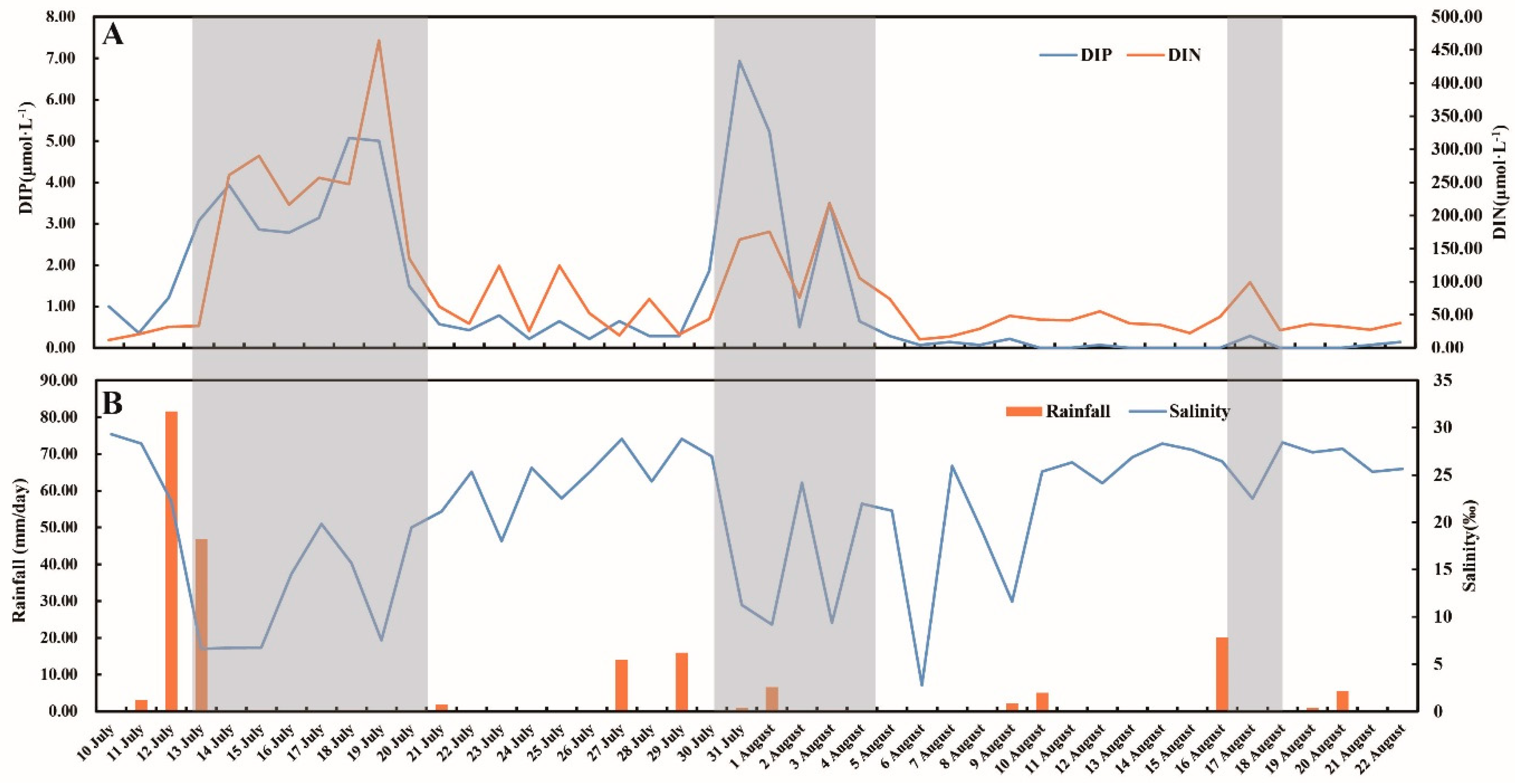
3.1. Environmental Factors

The values of the environmental factors are shown in Table A1. For nutrients, the concentrations of DIN, NH4, NO3, and NO2 were in the ranges 27.50–871.42 μmol·L−1, 0.57–61.14 μmol·L−1, 4.00–435.00 μmol·L−1, and 0.21–8 μmol·L−1, respectively, and the concentrations of DIP and silicate were in the ranges 0–6.93 μmol·L−1 and 27.5–871.43 μmol·L−1, respectively. More importantly, the level of N/P was always higher than the Redfield value (16:1) [24] in this area. For physical parameters, the value of DO, temperature, and pH were in ranges 6.05–13.81%, 24.4–31.1 °C, and 7.64–8.62, respectively (Table A1). The salinity value varied greatly, ranging from 2.77 to 29.31‰ (Table A1).
Further, different types of nutrients showed a significant correlation with each other (Figure 2). For example, the concentration of DIP showed a significant (p < 0.05) positive correlation with that of other nutrients, i.e., NH4, NO3, NO2, DIN, and silicate (Figure 2). It is notable that the levels of DIP and DIN increased (Figure A1A) with the salinity decreasing (Figure A1B). Meanwhile, the level of salinity was observed to manifest a significant (p < 0.01) negative correlation with all types of nutrients (Figure 2).

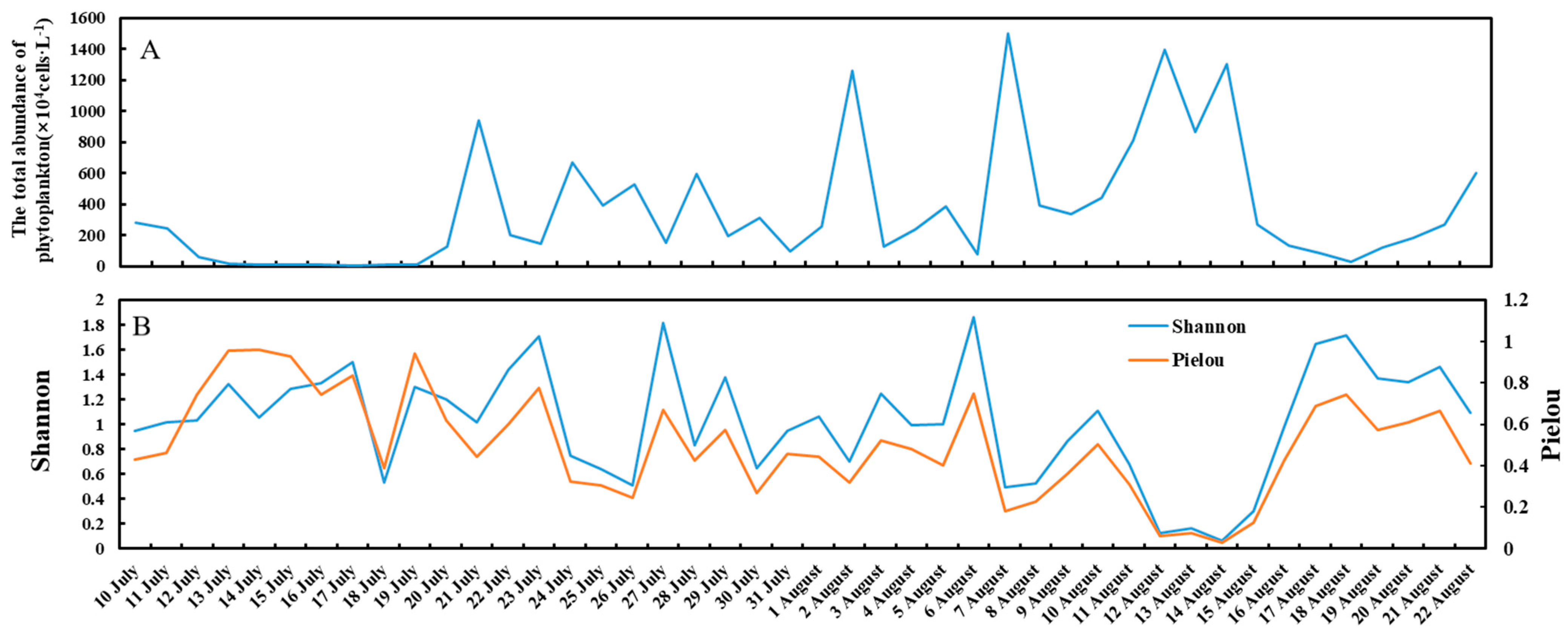
3.2. Total Abundance and Diversity of the Phytoplankton

The total abundance of phytoplankton ranged from 5.3 × 10⁴ to 1.5 × 10⁷ cells·L−1 (Figure 3A). In 12 July 2021–19 July 2021, the total abundance of phytoplankton was extremely low (with the value ranging from 5.3 × 10⁴ to 6.3 × 10⁵ cells·L−1) compared to data collected on other days of this study.
A total of 43 species were detected in Jinmeng Bay during our observation period, and all of those species belonged to three phyla: Bacillariophyta, Chromophyta, and Dinophyta (Table A2). Among those species, 27, 13, and 3 species belonged to Bacillariophyta, Dinophyta, and Chromophyta, respectively. It was clear that more species belonged to Bacillariophyta than the other two phyla. In addition, there were six most frequently detected species, i.e., Thalassiosira pacifica (T. pacifica), Skeletonema costatum (S. costatum), Chattonella marina (C. marina), Prorocentrum sigmoides (P. sigmoides), Pseudo-nitzschia delicatissima (P. delicatissima), and Nitzschia spp., which were detected in more than half of the samples. T. pacifica, S. costatum, P. delicatissima, and Nitzschia spp. belonged to Bacillariophyta, with detectable rates equal to 52.3%, 75%, 84.1%, and 72.7%, respectively. C. marina and P. sigmoides belonged to Chromophyta and Dinophyta, respectively, at a 65.9% and 56.8% detectable rate, respectively. It was notable that five species, i.e., C. marina, Heterosigma akashiwo (H. akashiwo), Gymnodinium catenatum (G. catenatum), Alexandrium catenella (A. catenella), and Akashiwo sanguinea (A. sanguinea) were identified as toxic species according to the “Technical specification for red tide monitoring in China”.
The Shannon diversity and Pielou evenness index showed the same trend and varied from 0.07 to 1.86 and 0.03 to 0.96, respectively (Figure 3B). The varied diversity demonstrated the shift in the phytoplankton community structure and rapid succession of the phytoplankton community. The lowest diversity (both Shannon diversity and Pielou evenness) occurred from 11 August 2021 to 14 August 2021, implying an unstable community structure during this period. It was also notable that the value of the diversity (i.e., the Shannon diversity and the Pielou evenness index) declining to the bottom corresponded to the total abundance of phytoplankton reaching the peaks, and significant (p < 0.001) negative correlations were also observed between the total phytoplankton abundance and the value of diversity (i.e., the Shannon diversity and the Pielou evenness index). These results demonstrated that the bloom of one species would occupy the niche of other phytoplankton species and decrease the diversity, which broke down the ecological balance in this area.

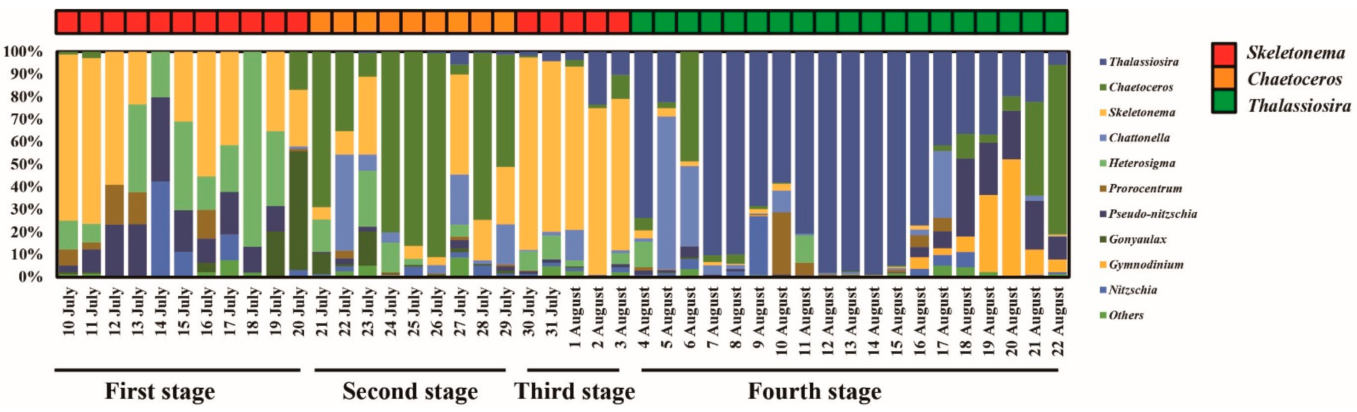
3.3. Phytoplankton Community

Generally speaking, Bacillariophyta was the most abundant phylum in all the samples except for 18 July 2021 and 5 August 2021, accounting for more than 85% of the total abundance (Figure 4). It is worth noting that only three species belonged to Chromophyta, while the abundance of Chromophyta accounted for 8.0% of the total abundance. Inversely, the abundance of Dinophyta accounted for 4.6% of the total abundance; 13 species belonging to this phylum were detected.
Further, non-metric multi-dimensional scaling (NMDS) analyses were carried out to reveal the shift in the phytoplankton community during this period (Figure 5). The results showed that all samples were clustered into A, B, and C groups, and significant (p < 0.01) differences were observed between each group (Table A3), demonstrating that the communities were distinct in those three groups.
To further reveal the subtle changes in the phytoplankton community composition in different groups, the community compositions of those samples were analyzed at the genus level (Figure 6). Consistent with the results of NMDS, the A, B, and C groups showed distinct community compositions and different genera predominated. In Group A, Skeletonema and Heterosigma were identified as the top two most abundant genera, accounting for 49.7–93.7% of the total abundance. Skeletonema was the predominant genus, detected in all samples and contributing to 56.4% of the total abundance in Group A. Meanwhile, Chaetoceros was identified as a major contributor (70.0%) to the relative abundance of the phytoplankton in Group B. Meanwhile, the phytoplankton communities were dominated by Thalassiosira in group C, which contributed 71% of the total abundance in this group.
Across the time series, the predominant genera showed a rapid succession during our observation period, and phytoplankton community compositions showed four stages. The phytoplankton compositions of the first (10 July 2021 to 20 July 2021) and third stages (30 July 2021 to 03 August 2021) belonged to group A and were dominated by Skeletonema. The phytoplankton compositions of the second (21 July 2021 to 29 July 2021) and fourth (4 August 2021 to 20 August 2021) stages pertained to Group B and C, respectively, and were dominated by Chaetoceros and Thalassiosira, respectively.
Overall, the phytoplankton communities were in constant succession during our observation of coastal waters of Qinhuangdao. Moreover, Skeletonema, Chaetoceros, and Thalassiosira were the predominant genera at different stages.

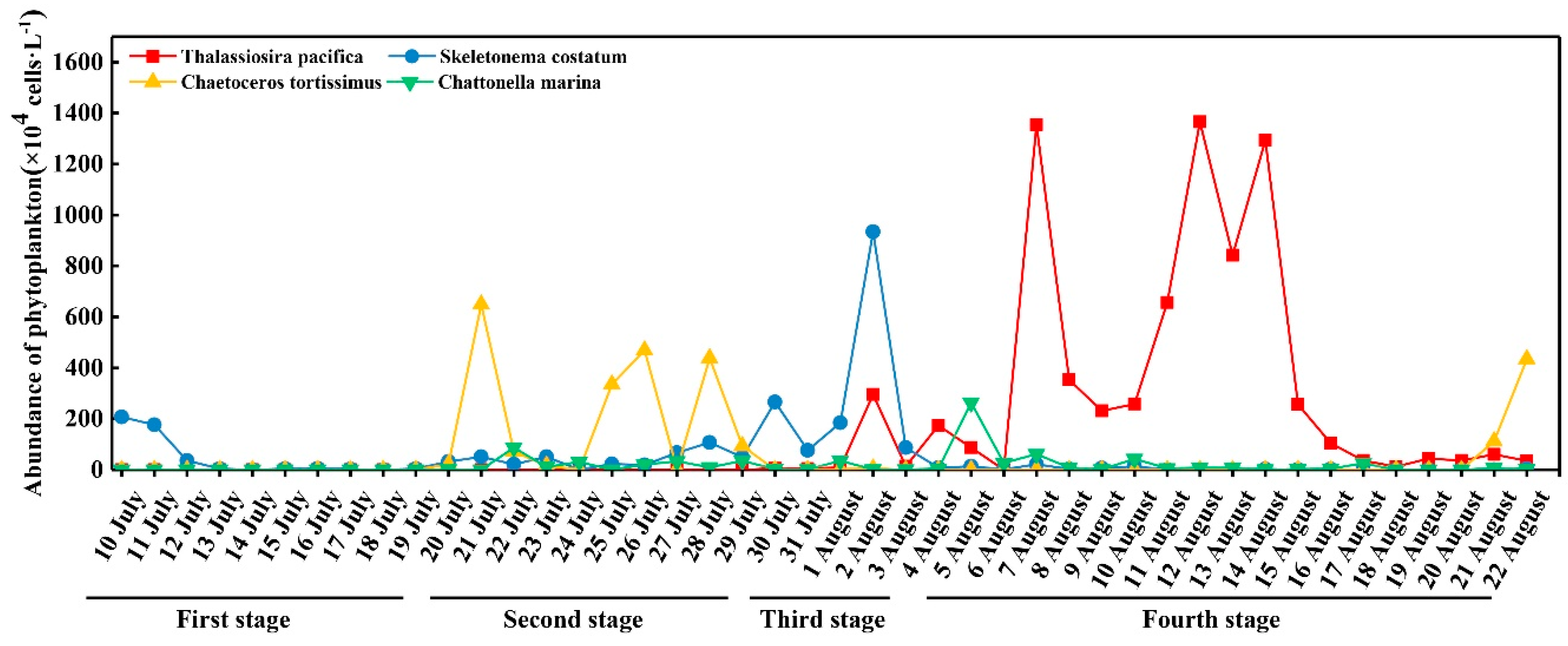
3.4. Abundance of Dominant Species

Of the total 43 species, four species—T. pacifica, S. costatum, Chaetoceros tortissimus (C. tortissimus), and C. marina—were identified as dominant species with Y > 0.02, and accounted for 83.87% of the total abundance. The abundance of T. pacifica, S. costatum, C. tortissimus, and C. marina was in the range 0–1.27 × 10⁷ cells·L−1, 0–9.34 × 10⁶ cells·L−1, 0–6.49 × 10⁶ cells·L−1, and 0–3.64 × 10⁶ cells·L−1, respectively (Figure 7). Interestingly, the top three dominant species did not show invariably high abundance during our observation time. Similarly to the community composition, the abundance of phytoplankton could also be split into four stages. A low abundance of four dominant species was observed in the first stage compared to the other stages. In the second stage, C. tortissimus bloomed from 21 July 2021 to 29 July 2021, with an average abundance of 2.5 × 10⁶ cells·L−1. S. costatum showed a short bloom from 30 July 2021 to 03 August 2021 in the third stage. Finally, the abundance of T. pacifica (with an average value of 4.2 × 10⁷ cells·L−1) bloomed from 4 August 2021 to 20 August 2021 in the fourth stage. It was notable that the abundance of T. pacifica covered the threshold value (2.0 × 10⁵ cells·L−1) of red tide for 20 days according to the “Technical specification for red tide monitoring in China” [20], suggesting that a persistent T. pacifica red tide broke out in this area.
Overall, T. pacifica, S. costatum, C. tortissimus, and C. marina were the dominant species during observations in Qinhuangdao coastal water. Meanwhile, the top three dominant species blooms predominated the succession of the phytoplankton community.

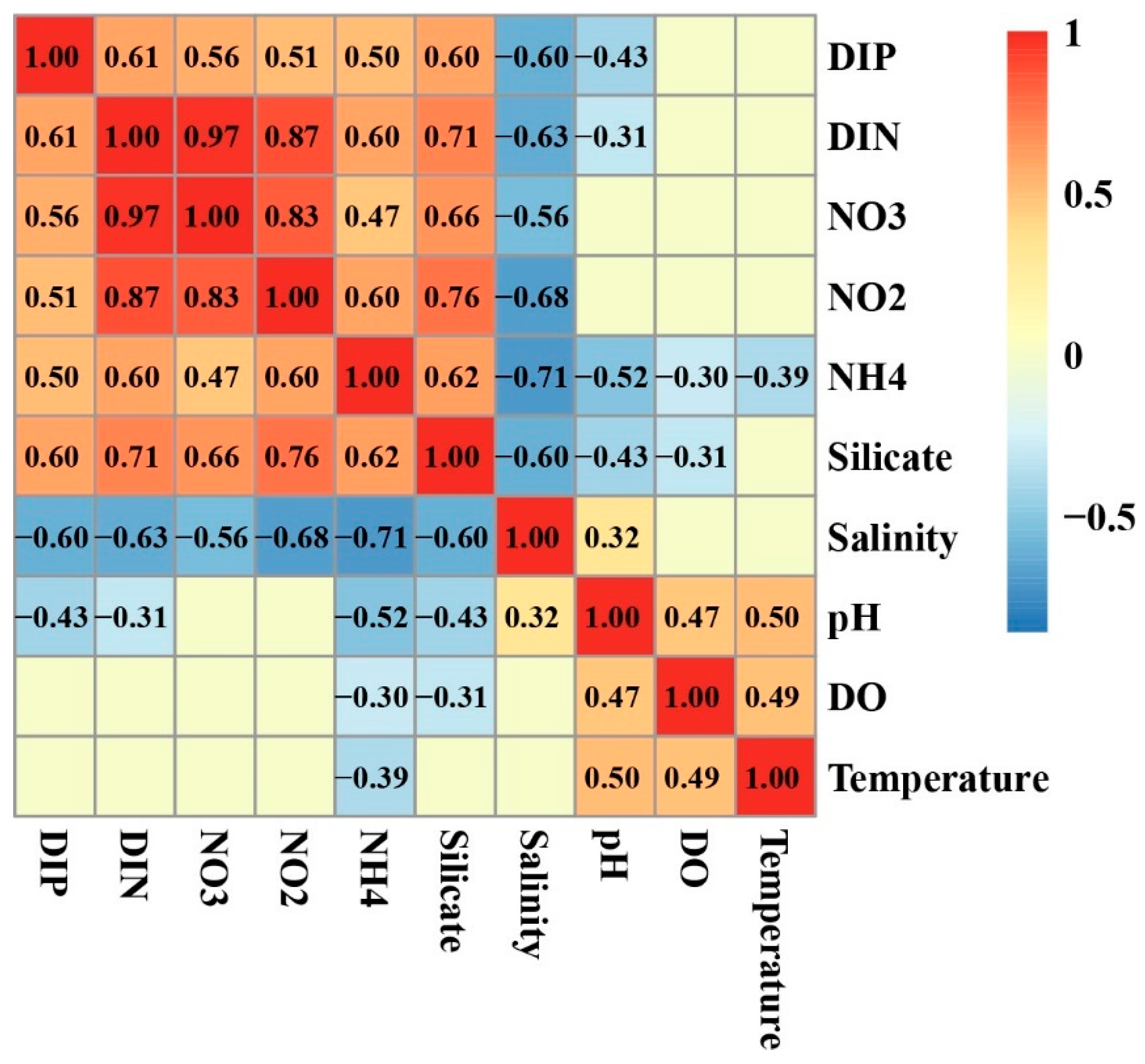
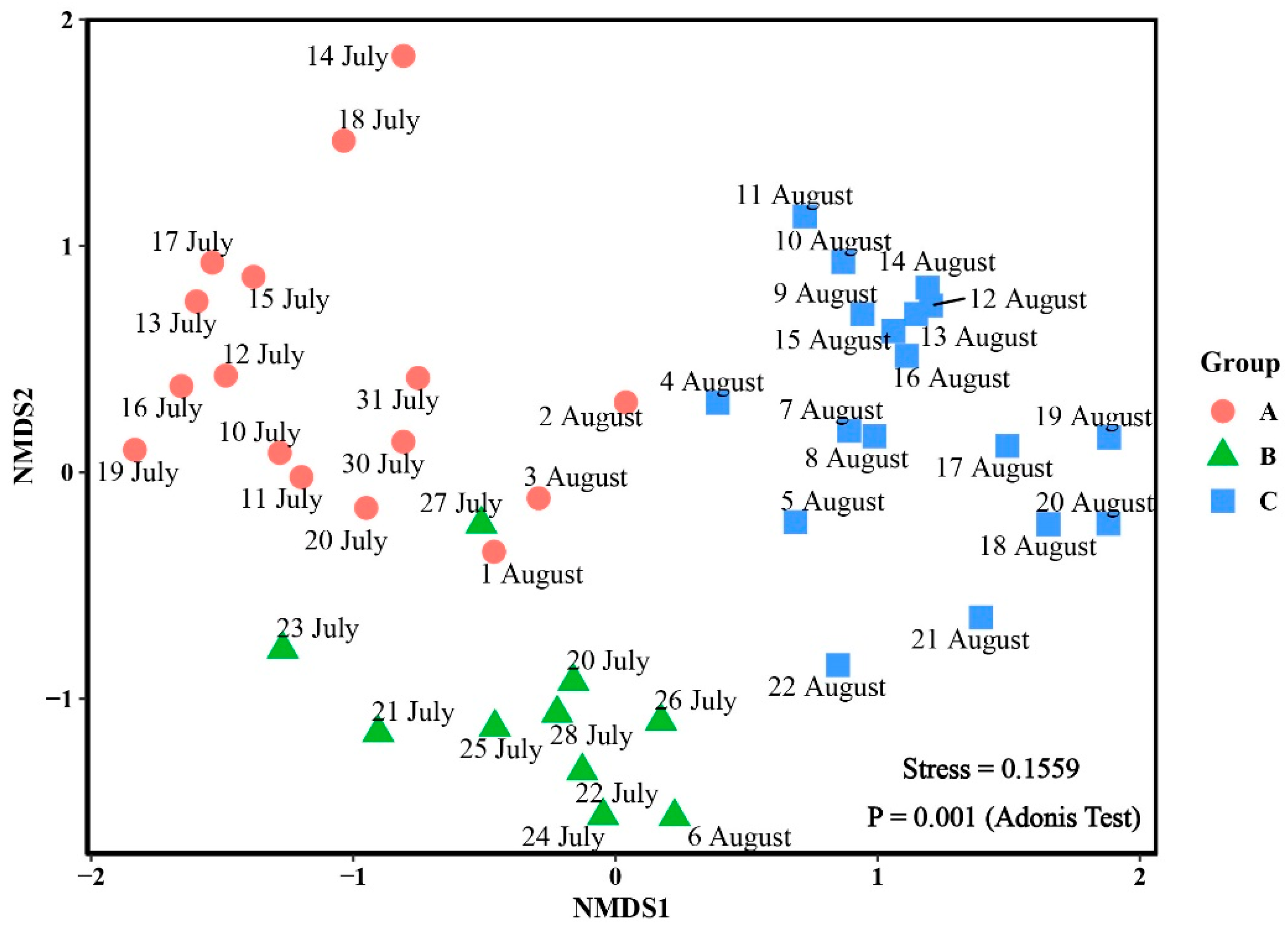
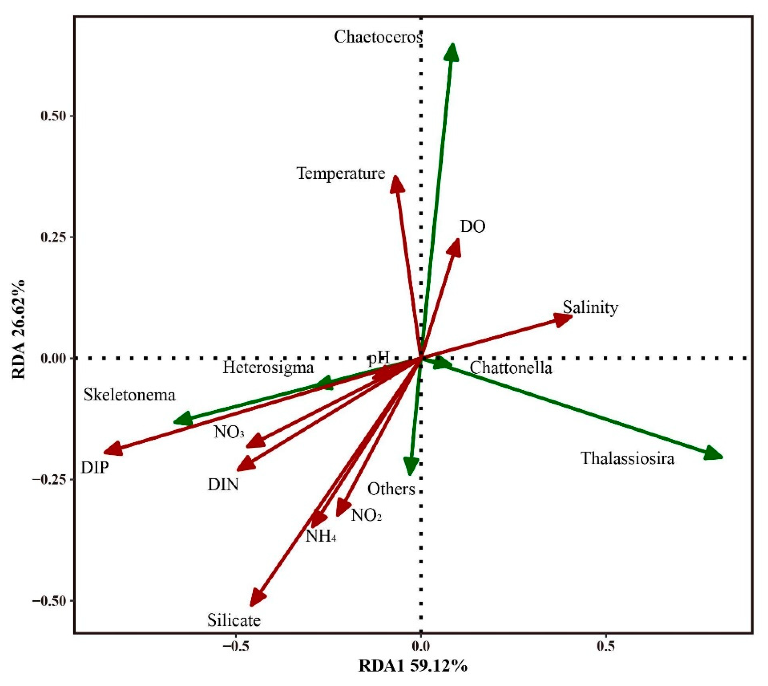
3.5. Relationship of Environmental Factors with Phytoplankton Abundance and Community Structure

A redundancy analysis (RDA) was employed to understand the relationship of environmental factors with the phytoplankton community (Figure 8). The first two axes explained 59.12% and 26.62% of the cumulative variance in the species–environmental variables. Based on the intersect correlation of environmental variables with the RDA axis, DIP (r = −0.853) and silicate (r = −0.509) were strongly related to axis 1 and axis 2, respectively. The Mantel test also showed that a range of environmental factors, including NH4, NO3, DIP, salinity, pH, temperature, and DIN, were significantly (p < 0.05) correlated with the phytoplankton community. DIP showed the highest correlation with the phytoplankton community among all the environmental factors (Table A4). Thus, we concluded that DIP was the most important environmental factor in the shift in phytoplankton community structure in the research area.
Furthermore, we analyzed the correlation between environmental factors and four dominant species (Table A5). The results showed that the level of DIP was negatively (p < 0.05) correlated with the abundance of T. pacifica and C. marina and positively (p < 0.05) correlated with S. costatum. Moreover, the abundance of C. tortissimus was observed to significantly correlate with the temperature levels. Overall, the DIP level was significantly associated with changes in the phytoplankton community and correlated with the bloom of T. pacifica, C. marina, and S. costatum in the Qinhuangdao coast.

4. Discussion

4.1. Inflows Facilitating the Rapid Succession of Phytoplankton

Freshwater inflow pulses are mostly characterized by the increase in nutrients in coastal waters, the rapid change in salinity, and the horizontal displacement of organisms [25]. Consistent with these findings, our research also found that the level of salinity ranged from 2.77 to 29.31‰ and was negatively correlated to the nutrients, suggesting that increased inflows enhanced the nutrients in coastal water. Meanwhile, we observed that Skeletonema costatum dominated the phytoplankton community during two stages, i.e., the first stage and the third stage, which were with relative low salinity and high level of nutrients (Figure A1A,B). Previous studies have demonstrated that an environment with abundant nutrients is suitable for the bloom of Skeletonema costatum [26,27]. Considering that the Skeletonema costatum was a marine species [28] and was hardly detected in fresh waters, we speculated that the Skeletonema costatum cannot be taken into coastal waters from the upper river. Thus, we think that the enhanced inflows facilitate the growth of Skeletonema costatum, which was the main contributor to total phytoplankton abundance in the first and third stages. Notably, although Skeletonema costatum dominated the phytoplankton community in first stage, the abundance of Skeletonema costatum was lowest compared to other stages. This can be ascribed to inflows diluting the abundance of Skeletonema costatum and facilitating its clone.
As a response to these excess nutrients, the phytoplankton community was in constant succession according to the daily sampling results. These results agreed with a number of previous studies, which found that inflows influenced the phytoplankton community in America, South Africa, Malaysia, and the Eastern Mediterranean based on weekly and monthly data [15,29,30]. However, our results found that the succession of the phytoplankton community was rapid. For example, the community dominated by Skeletonema in the third stage only persisted for 5 days, and it would take fewer than 3 days, sometimes only 1 day, to transform from one community composition to another community composition, which was consistent with the results from a microcosm experiment showing that the phytoplankton community had changed in 1 day by the addition of nutrients [31]. Clearly, we found that phytoplankton succession was rapid in coastal waters affected by inflows and recommended to capture the details of phytoplankton community shifts using hourly sampling.
Inflows also affected the phytoplankton community by physical interaction [29]. Phytoplankton exhibits a striking diversity in cell shapes and characteristics, which may influence its kinematics in important ways. The observed polymorphism of phytoplankton implies large morphological changes over demographic timescales, such as the reversible loss of horns or spines or changes in chain formation, which can modify to change their movement behavior [32]. Recent research indicated that phytoplankton were capable of precise control over their movement and behavior through the fine-scale control of cellular morphology [33]. Thus, some phytoplankton species are easily diluted by inflows; therefore, the phytoplankton community is significantly changed [33,34]. However, due to the lack of hydrodynamic data, in the present study we could not quantitatively estimate the influence of hydrodynamic forcing, including inflows and tides, on phytoplankton. Future works are recommended to investigate this problem based on numerical modeling to comprehensively understand the influence of inflow on phytoplankton in coastal waters.
In this study, inflows facilitated phytoplankton community succession, with the dominant genera changing in the order of SkeletonemaChaetocerosSkeletonemaThalassiosira. Blooms and related changes in phytoplankton composition were accompanied by loss of fish and invertebrate populations and altered food web processes [35,36,37]. Moreover, the succession of phytoplankton could significantly influence the bacterial community, which may further change ecosystem functioning [38].
Overall, our results provide a high-temporal-resolution observation of the succession of phytoplankton community and show that changes in inflows facilitate the rapid phytoplankton community succession. Our findings help to understand the shift in the phytoplankton community in coastal waters.

4.2. DIP and the Bloom of Phytoplankton

Phosphorus (P) is one of the vital macronutrients utilized by phytoplankton. As such, phosphorus availability exerts imperative control over oceanic primary production [39,40,41,42,43]. Phytoplankton can effortlessly transport and assimilate dissolved inorganic phosphorus (DIP) directly into needed biomolecules, making this their favored form of phosphorus [44]. In this study, the level of DIP was significantly associated with shifts in the phytoplankton community and the blooms of T. pacifica, C. marina, and S. costatum on the Qinhuangdao coast, which aligns with a number of field studies in this area [45,46].
In this study, the level of DIP was negatively correlated with the abundance of T. pacifica, which had the highest dominance among all species. We found that T. pacifica bloomed during the lowest level of DIP, the concentration of which was even lower than the detection limit. This result could be due to Thalassiosira sp. being well suited to low DIP environments. Compared to other phytoplankton, Thalassiosira sp. is less sensitive to the level of DIP [47]. Further experiments based on genomics and transcriptomics reveal that Thalassiosira sp. shows multiple response mechanisms to ambient P-deficiency [41,48]. These can not only redistribute cellular phosphorus but also acquire phosphorus from organic compounds through increasing the expression of various phosphatases [41]. Additionally, Thalassiosira sp. also uses non-P lipids, such as sulfolipids (sulfur-containing) and betaine lipids (N-containing), to replace P-containing lipids [48,49].
S. costatum was the second most dominant species, the abundance of which was positively correlated with levels of DIP and dominated the phytoplankton community during the high concentration of nutrients (Figure 4 and Figure A1). This result is consistent with findings in a previous study at a bay of Xiamen, Fujian Province, China [50]. Additionally, laboratory experiments found that the growth of S. costatum is sensitive to the level of DIP, which positively correlates with inorganic carbon acquisition abilities [51]. Thus, a high concentration of DIP facilitated the bloom of S. costatum.
Overall, DIP showed a correlation with the bloom of the top two dominant species, i.e., T. pacifica and S. costatum, in our research area. The results contribute to our present understanding of the occurrence of phytoplankton bloom and are beneficial for the development of management strategies for controlling phytoplankton bloom in coastal waters.

4.3. The Potential Risk of Harmful Algal Blooms

Algae blooms usually change the environment of coastal waters significantly and can damage public health and the entire economy of the coastal region. In this study, we observed a persistent bloom of T. pacifica for 20 days. Although T. pacifica is a nontoxic species, its bloom significantly changes the water color and enhances the mortality of fish and shellfish in coastal regions by reducing the dissolved oxygen of seawater [52]. Additionally, the pathogens associated with Thalassiosira are resistant to environmental stress and may adversely affect the health of tourists [53]. Thus, the bloom of T. pacifica caused a terrible experience e.g., abnormal water color and potential risk of illness, for tourists in Jinmeng Bay. Additionally, T. pacifica bloom inhibits the reproduction of Pseudocalanus newmani [54], which may further disturb the ecological balance in this area.
Additionally, five toxic species, i.e., C. marina, H. akashiwo, G. catenatum, A. catenella, and A. sanguinea, were detected in this area. Among these five species, H. akashiwo, A. catenella, and A. sanguinea had a low concentration, but this does not mean that we can neglect the harm caused by these species. Unfortunately, the occurrence of these species demonstrated that the potential risk of the blooms of these species exists. It is notable that C. marina is not only a toxic species but also a dominant species in this area. C. marina has caused harmful algal blooms worldwide, associated with massive mortality for wild and cultivated fishes [55,56,57]. Respiratory deficiency is generally believed to be the direct cause of fish death by this toxic algal species [58,59]. Although the abundance of this algae only exceeded the threshold value (1.0 × 10⁶ cells·L−1) of the red tide for one day [20], it is a persistent species in this area and may also influence the survival of fishes. Overall, although there was no persistent bloom of toxic algae, the government should focus on the potential risk of toxic algae.

5. Conclusions

This study investigated the influence of environmental factors on day-to-day changes in phytoplankton during summer in Jinmeng Bay, Qinhuangdao. Phytoplankton communities displayed rapid succession with the predominant genera, changing in the order of SkeletonemaChaetocerosSkeletonemaThalassiosira. Similarly, T. pacifica, S. costatum, C. tortissimus, and C. marina were identified as dominant species. A persistent T. pacifica red tide outbroke for 20 days in this area. Moreover, inflows facilitated the rapid succession of the phytoplankton community, and DIP was identified as a key factor affecting the succession of the phytoplankton communities and blooms of the top three dominant species, i.e., T. pacifica, S. costatum, and C. tortissimus. Overall, our results provide high-temporal-resolution observations regarding the succession of the phytoplankton community and shed some light on the complex responses of phytoplankton to environmental factors. In the future, numerical modeling can be employed to simulate interactions among phytoplankton, nutrients, and hydrodynamic forces and to further build a pre-warning system of algae blooms.

Author Contributions

Conceptualization, Y.H. and Z.C.; methodology, Z.C. and X.F.; formal analysis and investigation, Y.H. and Z.C.; validation and data curation, Z.C.; writing—original draft preparation, Y.H.; writing—review and editing, G.W. (Guangyi Wang) and J.Z.; supervision and project administration, J.Z. and G.W. (Gang Wang); and funding acquisition, J.Z. All authors have read and agreed to the published version of the manuscript.

Funding

This research was funded by Key R&D Program of Hebei Province, China, 21373302D and National Key R&D Program of China, 2019YFC1407905.

Institutional Review Board Statement

Not applicable.

Informed Consent Statement

Not applicable.

Data Availability Statement

All data underlying the results are included as part of the published article.

Acknowledgments

The authors would like to thank the reviewers for insightful comments.

Conflicts of Interest

The authors declare no conflict of interest.

Appendix A

Figure A1. The level of DIN, DIP, salinity and rainfall in Qinhuangdao. Figure (A) presents the level of DIN and DIP; Figure (B) presents the level of salinity and rainfall. The shadow represents the period with relative low salinity.
Water 14 01625 g0a1
Table A1. Value of environmental factors in coastal waters in this study area during the study period.
Environmental FactorsMinimum ValueMaximum ValueMean ± SD
NH4 (μmol·L−1)0.5761.1411.35 ± 11.94
NO3 (μmol·L−1)4.00435.0077.26 ± 89.46
NO2 (μmol·L−1)0.218.002.48 ± 1.84
DIP (μmol·L−1)ND6.931.23 ± 1.77
Silicate (μmol·L−1)27.5871.43242.94 ± 185.71
DO (%)6.0513.818.84 ± 1.75
Salinity (‰)2.7729.3120.97 ± 7.58
pH7.648.628.10 ± 0.21
Temperature (°C)24.4031.1028.05 ± 1.76
DIN (μmol·L−1)27.50871.4291.09 ± 96.81
N/P23.894--
Note: “--” and “∞” represent no detected and infinity, respectively.
Table A2. The species identified during this period.
PhylumSpeciesDetectable Rate
BacillariophytaThalassiosira pacifica0.52
Skeletonema costatum0.75
Chaetoceros tortissimus0.30
Chaetoceros spp.0.41
Pseudo-nitzschia delicatissima0.84
Nitzschia spp.0.73
Leptocylindrus danicus0.05
Chaetoceros curvisetus0.34
Pseudo-nitzschia pungens0.16
Thalassionema nitzschioides0.20
Chaetoceros diadema0.11
Chaetoceros decipiens0.05
Thalassiosira spp.0.14
Licmophora abbreviata0.11
Chaetoceros lorenzianus0.14
Pinnularia spp.0.16
Thalassiothrix frauenfeldii0.02
Coscinodiscus spp.0.09
Detonula pumila0.09
Guinardia delicatula0.05
Thalassiosira nordenskioeldii0.02
Chaetoceros peruvianus0.02
Chaetoceros affinis0.07
Chaetoceros abnormis0.02
Hemiaulus sinensis0.02
Guinardia flaccida0.05
Nitzschia longissima0.02
DinophytaProrocentrum sigmoides0.57
Gymnodinium catenatum0.25
Gonyaulax verior0.18
Gonyaulax spp.0.20
Scrippsiella trochoidea0.27
Protoperidinium pellucidum0.27
Prorocentrum minimum0.11
Ceratium fusus0.11
Alexandrium catenella0.02
Ceratium tripos0.11
Karenia mikimotoi0.02
Akashiwo sanguinea0.02
Protoperidinium spp.0.02
ChromophytaChattonella marina0.66
Heterosigma akashiwo0.48
Dictyocha fibula0.11
Table A3. p value of pairwise comparisons for phytoplankton community using permutation MANOVAs.
GroupsAB
B0.001-
C0.0010.001
Table A4. The correlation between environmental factors and phytoplankton community based on Mantel test.
Environmental Factorsrp Value
NH40.099 *0.027
NO30.106 *0.01
NO20.0070.406
DIP0.287 **0.001
Silicate0.0470.133
DO0.0470.137
Salinity0.092 *0.022
pH0.085 *0.026
Temperature0.148 **0.001
DIN0.099 *0.022
Note: “*” and “**” represent significant correlation with p < 0.05 and p < 0.01, respectively.
Table A5. The Spearman correlation between environmental factors and abundance of dominant phytoplankton species.
Environmental FactorsThalassiosira pacificaSkeletonema costatumChaetoceros tortissimusChattonella marina
NH4−0.224−0.179−0.169−0.274
NO3−0.1600.1090.077−0.207
NO20.0390.034−0.004−0.117
DIP−0.620 **0.472 **0.070−0.306 *
Silicate−0.1060.101−0.189−0.305 *
DO0.1720.1750.2570.231
Salinity0.263−0.0100.0670.144
pH0.255−0.0810.2840.075
Temperature0.0280.1820.476 **0.288
DIN−0.1890.0720.058−0.259
Note: “*” and “**” represent significant correlation with p < 0.05 and p < 0.01, respectively.

References

  1. Falkowski, P.G.; Barber, R.T.; Smetacek, V. Biogeochemical controls and feedbacks on ocean primary production. Science 1998, 281, 200–206. [Google Scholar] [CrossRef] [PubMed] [Green Version]
  2. Arrigo, K. Marine microorganisms and global nutrient cycles. Nature 2005, 437, 349–355. [Google Scholar] [CrossRef] [PubMed]
  3. Hilligsøe, K.M.; Richardson, K.; Bendtsen, J.; SøRensen, L.L.; Nielsen, T.G.; Lyngsgaard, M.M. Linking phytoplankton community size composition with temperature, plankton food web structure and sea–air CO2 flux. Deep-Sea Res. Part I 2011, 58, 826–838. [Google Scholar] [CrossRef]
  4. Kroeze, C.; Hofstra, N.; Ivens, W.; Loehr, A.; Strokal, M.; Wijnen, J.V. The links between global carbon, water and nutrient cycles in an urbanizing world—The case of coastal eutrophication. Curr. Opin. Environ. Sustain. 2013, 5, 566–572. [Google Scholar] [CrossRef]
  5. Genitsaris, S.; Sommer, M.-G. Phytoplankton Blooms, Red Tides and Mucilaginous Aggregates in the Urban Thessaloniki Bay, Eastern Mediterranean. Diversity 2019, 11, 136. [Google Scholar] [CrossRef] [Green Version]
  6. Kouakou, C.R.; Poder, T.G. Economic impact of harmful algal blooms on human health: A systematic review. J. Water Health 2019, 17, 499–516. [Google Scholar] [CrossRef] [Green Version]
  7. Cira, E.K.; Palmer, T.A.; Wetz, M.S. Phytoplankton dynamics in a low-inflow estuary (Baffin Bay, TX) during drought and high-rainfall conditions associated with an El Niño event. Estuaries Coasts 2021, 44, 1752–1764. [Google Scholar] [CrossRef]
  8. Kotsedi, D.; Adams, J.B.; Snow, G.C. The response of microalgal biomass and community composition to environmental factors in the Sundays Estuary. Water 2012, 38, 177–190. [Google Scholar] [CrossRef] [Green Version]
  9. Kaselowski, T. Not so pristine-characterising the physico-chemical conditions of an undescribed temporarily open/closed estuary. Water 2013, 39, 627–635. [Google Scholar] [CrossRef] [Green Version]
  10. Buyukates, Y.; Roelke, D. Influence of pulsed inflows and nutrient loading on zooplankton and phytoplankton community structure and biomass in microcosm experiments using estuarine assemblages. Hydrobiologia 2005, 548, 233–249. [Google Scholar] [CrossRef]
  11. Hylén, A.; van de Velde, S.J.; Kononets, M.; Luo, M.; Almroth-Rosell, E.; Hall, P.O. Deep-water inflow event increases sedimentary phosphorus release on a multi-year scale. Biogeosciences 2021, 18, 2981–3004. [Google Scholar] [CrossRef]
  12. Wachnicka, A.; Browder, J.; Jackson, T.; Louda, W.; Kelble, C.; Abdelrahman, O.; Stabenau, E.; Avila, C. Hurricane Irma’s impact on water quality and phytoplankton communities in Biscayne Bay (Florida, USA). Estuaries Coasts 2020, 43, 1217–1234. [Google Scholar] [CrossRef]
  13. Cui, L.; Lu, X.; Dong, Y.; Cen, J.; Cao, R.; Pan, L.; Lu, S.; Ou, L. Relationship between phytoplankton community succession and environmental parameters in Qinhuangdao coastal areas, China: A region with recurrent brown tide outbreaks. Ecotoxicol. Environ. Saf. 2018, 159, 85–93. [Google Scholar] [CrossRef] [PubMed]
  14. Sin, Y.; Yu, H. Phytoplankton community and surrounding water conditions in the Youngsan River estuary: Weekly variation in the saltwater zone. Ocean Polar Res. 2018, 40, 191–202. [Google Scholar]
  15. Nunes, M.; Adams, J.B.; Rishworth, G.M. Shifts in phytoplankton community structure in response to hydrological changes in the shallow St Lucia Estuary. Mar. Pollut. Bull. 2018, 128, 275–286. [Google Scholar] [CrossRef]
  16. Tao, J.-H. Numerical simulation of aquatic eco-environment of Bohai Bay. J. Hydrodyn. Ser. B 2006, 18, 34–42. [Google Scholar] [CrossRef]
  17. Zhang, Y.; Li, X.; Zhang, W.; Zhang, J. Spatial and temporal distribution of silicate and chlorophyll a in the coastal waters with picophytoplankton algal bloom. Ecol. Sci. 2013, 32, 509–513. [Google Scholar]
  18. He, Y.; He, Y.; Sen, B.; Li, H.; Li, J.; Zhang, Y.; Zhang, J.; Jiang, S.C.; Wang, G. Storm runoff differentially influences the nutrient concentrations and microbial contamination at two distinct beaches in northern China. Sci. Total Environ. 2019, 663, 400–407. [Google Scholar] [CrossRef]
  19. GB/T 12763-2007; General Administration of Quality Supervision, Inspection and Quarantine of the People’s Republic of China. Specification for the Oceanographic Survey. China National Standardization Management Committee: Beijing, China, 2007.
  20. HY/T 069-2005; State Oceanic Administration (SOA). Technical Specification for Red Tide Monitoring in China. China National Standardization Management Committee: Beijing, China, 2005.
  21. Utermöhl, H. Zur vervollkommnung der quantitativen phytoplankton-methodik: Mit 1 Tabelle und 15 abbildungen im Text und auf 1 Tafel. Int. Ver. Für Theor. Und Angew. Limnol. Mitt. 1958, 9, 1–38. [Google Scholar] [CrossRef]
  22. Team, R.C. R: A language and environment for statistical computing. Computing 2011, 1, 12–21. [Google Scholar]
  23. Ji, F.; Sun, Y.; Ma, Q.; Feng, X.; Mi, D. Response of planktonic communities to environmental stress in the eutrophic waters of Xiaoping Island in China. Chemosphere 2021, 275, 130107. [Google Scholar] [CrossRef] [PubMed]
  24. Redfield, A. The biological control of chemical factors in the environment. Am. Sci. 1958, 46, 205–221. [Google Scholar]
  25. Hemraj, D.A.; Hossain, A.; Ye, Q.; Qin, J.G.; Leterme, S.C. Anthropogenic shift of planktonic food web structure in a coastal lagoon by freshwater flow regulation. Sci. Rep. 2017, 7, 44441. [Google Scholar] [CrossRef] [Green Version]
  26. Li, C.; Zhu, B.; Chen, H.; Liu, Z.; Cui, B.; Wu, J.; Li, B.; Yu, H.; Peng, M. The relationship between the Skeletonema costatum red tide and environmental factors in Hongsha Bay of Sanya, South China Sea. J. Coast. Res. 2009, 25, 651–658. [Google Scholar] [CrossRef]
  27. Samuels, W.B.; Kleppel, G.S.; McLaughlin, J.J. Population growth patterns of Skeletonema costatum and nutrient levels in the lower East River, New York, USA. Hydrobiologia 1983, 98, 35–43. [Google Scholar] [CrossRef]
  28. Cleve, P.T. Examination of diatoms found on the surface of the Sea of Java. Bih. Kongl. Sven. Vet-Akad. Handl. 1873, 1, 1–13. [Google Scholar]
  29. Roelke, D.L.; Spatharis, S. Phytoplankton succession in recurrently fluctuating environments. PLoS ONE 2015, 10, e0121392. [Google Scholar] [CrossRef] [Green Version]
  30. Chong, B.; Leong, S.; Kuwahara, V.S.; Yoshida, T. Monsoonal variation of the marine phytoplankton community in Kota Kinabalu, Sabah. Reg. Stud. Mar. Sci. 2020, 37, 101326. [Google Scholar] [CrossRef]
  31. Zhang, C.; Yao, X.; Chen, Y.; Chu, Q.; Yu, Y.; Shi, J.; Gao, H. Variations in the phytoplankton community due to dust additions in eutrophication, LNLC and HNLC oceanic zones. Sci. Total Environ. 2019, 669, 282–293. [Google Scholar] [CrossRef]
  32. Zohdi, E.; Abbaspour, M. Harmful algal blooms (red tide): A review of causes, impacts and approaches to monitoring and prediction. Int. J. Environ. Sci. Technol. 2019, 16, 1789–1806. [Google Scholar] [CrossRef]
  33. Sengupta, A.; Carrara, F.; Stocker, R. Phytoplankton can actively diversify their migration strategy in response to turbulent cues. Nature 2017, 543, 555–558. [Google Scholar] [CrossRef] [PubMed]
  34. Li, F.; Zhang, H.; Zhu, Y.; Xiao, Y.; Chen, L. Effect of flow velocity on phytoplankton biomass and composition in a freshwater lake. Sci. Total Environ. 2013, 447, 64–71. [Google Scholar] [CrossRef] [PubMed]
  35. Livingston, R.J. Phytoplankton bloom effects on a gulf estuary: Water quality changes and biological response. Ecol. Appl. 2007, 17, S110–S128. [Google Scholar] [CrossRef]
  36. Imai, I. Ecophysiology, life cycle, and bloom dynamics of Chattonella in the Seto Inland Sea, Japan. Physiol. Ecol. Harmful Algal Bloom. 1998, 2, 71–84. [Google Scholar]
  37. Al Gheilani, H.M.; Matsuoka, K.; AlKindi, A.Y.; Amer, S.; Waring, C. Fish kill incidents and harmful algal blooms in Omani waters. J. Agric. Mar. Sci. 2011, 16, 23–33. [Google Scholar] [CrossRef] [Green Version]
  38. Mühlenbruch, M.; Grossart, H.P.; Eigemann, F.; Voss, M. Mini-review: Phytoplankton-derived polysaccharides in the marine environment and their interactions with heterotrophic bacteria. Environ. Microbiol. 2018, 20, 2671–2685. [Google Scholar] [CrossRef] [PubMed] [Green Version]
  39. Benitez-Nelson, C.R. The biogeochemical cycling of phosphorus in marine systems. Earth-Sci. Rev. 2000, 51, 109–135. [Google Scholar] [CrossRef]
  40. Ammerman, J.W.; Hood, R.R.; Case, D.A.; Cotner, J.B. Phosphorus deficiency in the Atlantic: An emerging paradigm in oceanography. Eos Trans. Am. Geophys. Union 2003, 84, 165. [Google Scholar] [CrossRef]
  41. Dyhrman, S.T.; Jenkins, B.D.; Rynearson, T.A.; Saito, M.A.; Mercier, M.L.; Harriet, A.; Whitney, L.P.; Andrea, D.; Bulygin, V.V.; Bertrand, E.M. The Transcriptome and Proteome of the Diatom Thalassiosira pseudonana Reveal a Diverse Phosphorus Stress Response. PLoS ONE 2012, 7, e33768. [Google Scholar] [CrossRef] [Green Version]
  42. Mather, R.L.; Reynolds, S.E.; Wolff, G.A.; Williams, R.G.; Torres-Valdes, S.; Woodward, E.; Landolfi, A.; Pan, X.; Sanders, R.; Achterberg, E.P. Phosphorus cycling in the North and South Atlantic Ocean subtropical gyres. Nat. Geosci. 2008, 1, 439–443. [Google Scholar] [CrossRef]
  43. Lomas, M.W.; Burke, A.; Lomas, D.; Bell, D.; Shen, C.; Dyhrman, S.T.; Ammerman, J.W. Sargasso Sea phosphorus biogeochemistry: An important role for dissolved organic phosphorus (DOP). Biogeosciences 2010, 7, 695–710. [Google Scholar] [CrossRef] [Green Version]
  44. Whitney, L.A.P.; Lomas, M.W. Phosphonate utilization by eukaryotic phytoplankton. Limnol. Oceanogr. Lett. 2019, 4, 18–24. [Google Scholar] [CrossRef] [Green Version]
  45. Zhang, J.L.; Wang, Q.Y.; Zhang, Y.F.; Zhang, W.L.; Li, L. Characteristics of seawater nutrients during the occurrence of brown tide in the coastal area of Qinhuangdao, China. Ying Yong Sheng Tai Xue Bao J. Appl. Ecol. 2020, 31, 282–292. [Google Scholar]
  46. Wang, Y.; Sun, Y.; Wang, C.; Chen, W.; Hu, X. Net-phytoplankton community structure and its environmental correlations in central Bohai Sea and the Bohai Strait. Aquat. Ecosyst. Health Manag. 2019, 22, 481. [Google Scholar] [CrossRef]
  47. Zhuming; Lian, Y. Research on the Nitrogen and Phosphorus Requirement of Thalassiosira sp. J. Aquac. 2004, 1, 33–36. [Google Scholar]
  48. Chen, X.-H.; Li, Y.-Y.; Zhang, H.; Liu, J.-L.; Xie, Z.-X.; Lin, L.; Wang, D.-Z. Quantitative proteomics reveals common and specific responses of a marine diatom Thalassiosira pseudonana to different macronutrient deficiencies. Front. Microbiol. 2018, 9, 2761. [Google Scholar] [CrossRef]
  49. Mooy, B.V.; Fredricks, H.F.; Pedler, B.E.; Dyhrman, S.T.; Karl, D.M.; Koblížek, M.; Lomas, M.W.; Mincer, T.J.; Moore, L.R.; Moutin, T. Phytoplankton in the ocean use non-phosphorus lipids in response to phosphorus scarcity. Nature 2009, 458, 69. [Google Scholar] [CrossRef]
  50. Yu, L.; Rong-cheng, L. Research on red tide occurrences using enclosed experimental ecosystem in West Xiamen Harbor, China—Relationship between nutrients and red tide occurrence. Chin. J. Oceanol. Limnol. 2000, 18, 253–259. [Google Scholar] [CrossRef]
  51. Gao, G.; Xia, J.; Yu, J.; Fan, J.; Zeng, X. Regulation of inorganic carbon acquisition in a red tide alga (Skeletonema costatum): The importance of phosphorus availability. Biogeosciences 2018, 15, 4871–4882. [Google Scholar] [CrossRef] [Green Version]
  52. Anderson, D.M.; Fensin, E.; Gobler, C.J.; Hoeglund, A.E.; Hubbard, K.A.; Kulis, D.M.; Landsberg, J.H.; Lefebvre, K.A.; Provoost, P.; Richlen, M.L. Marine harmful algal blooms (HABs) in the United States: History, current status and future trends. Harmful Algae 2021, 102, 101975. [Google Scholar] [CrossRef]
  53. Shetye, S.S.; Bandekar, M.; Nandakumar, K.; Kurian, S.; Gauns, M.; Jawak, S.; Pratihary, A.; Elangovan, S.S.; Naik, B.R.; Lakshmi, S. Sea foam-associated pathogenic bacteria along the west coast of India. Environ. Monit. Assess. 2021, 193, 27. [Google Scholar] [CrossRef] [PubMed]
  54. Halsband-Lenk, C.; Pierson, J.J.; Leising, A.W. Reproduction of Pseudocalanus newmani (Copepoda: Calanoida) is deleteriously affected by diatom blooms—A field study. Prog. Oceanogr. 2005, 67, 332–348. [Google Scholar] [CrossRef]
  55. Yuzao, Q.; Changjiang, H. The causative mechanism of Chatonella marina bloom in Dapeng Bay, the South China Sea. Oceanol. Limnol. Sin. 1997, 28, 337–342. [Google Scholar]
  56. Hallegraeff, G. Chattonella marina raphidophyte bloom associated with mortality of cultured bluefin tuna (Thunnus maccoyii) in South Australia. Harmful Algae 1998, 105, 414–417. [Google Scholar]
  57. Landsberg, J.H. The effects of harmful algal blooms on aquatic organisms. Rev. Fish. Sci. 2002, 10, 113–390. [Google Scholar] [CrossRef]
  58. Ishimatsu, A.; Maruta, H.; Oda, T.; Ozaki, M. A comparison of physiological responses in yellowtail to fatal environmental hypoxia and exposure to Chattonella marina. Fish. Sci. 1997, 63, 557–562. [Google Scholar] [CrossRef] [Green Version]
  59. Lee, K.; Ishimatsu, A.; Sakaguchi, H.; Oda, T. Cardiac output during exposure to Chattonella marina and environmental hypoxia in yellowtail (Seriola quinqueradiata). Mar. Biol. 2003, 142, 391–397. [Google Scholar] [CrossRef]
Figure 1. A map of the sampling station.
Water 14 01625 g001
Figure 2. The heatmap reveals the correlation between different environmental factors. The environmental factors were clustered using the parameter that method = “complete”. The color and number in the boxes show the level of r. All the boxes with numbers show a significant correlation, with p < 0.05.
Water 14 01625 g002
Figure 3. The day-to-day variations in total abundance of phytoplankton (A) and diversity (B).
Water 14 01625 g003
Figure 4. The community composition of phytoplankton at the phylum level in different samples.
Water 14 01625 g004
Figure 5. The non-metric multi-dimensional scaling (NMDS) reveals different phytoplankton communities based on the Euclidean distance in this period. The relative abundance of phytoplankton was used to calculate the Euclidean distance. Circles, triangles and squares, and crosses represent groups A, B, and C, respectively.
Water 14 01625 g005
Figure 6. The community composition of phytoplankton at genus level in different samples. The red, orange, and green boxes at the top represent samples that belong to Groups A, B, and C, respectively.
Water 14 01625 g006
Figure 7. The abundance of four dominant species in Qinhuangdao coastal water.
Water 14 01625 g007
Figure 8. A redundancy analysis (RDA) showing the relative abundance of different genera and environmental parameters. Green arrows and red arrows represent phytoplankton genera and environmental factors, respectively.
Water 14 01625 g008
Publisher’s Note: MDPI stays neutral with regard to jurisdictional claims in published maps and institutional affiliations.

