
Use of Heating Configuration to Control Marangoni Circulation during Droplet Evaporation


1
LR01ES07 Laboratoire d’Energétique et des Transferts Thermique et Massique de Tunis, Faculté des Sciences de Tunis, Université de Tunis El Manar, Tunis 2092, Tunisia
2
Faculté des Sciences de Bizerte, Université de Carthage, Bizerte 7021, Tunisia
3
Department of Engineering, University of Palermo, 90128 Palermo, Italy
4
Lehrstuhl fuer Hydromechanik & Hydrosystemmodellierung, Universitaet Stuttgart, 70569 Stuttgart, Germany
5
CentraleSupélec, Laboratoire de Génie des Procédés et Matériaux, SFR Condorcet FR CNRS 3417, Centre Européen de Biotechnologie et de Bioéconomie (CEBB), Université Paris-Saclay, 3 Rue des Rouges Terres, 51110 Pomacle, France
*
Author to whom correspondence should be addressed.
Water 2022, 14(10), 1653; https://0-doi-org.brum.beds.ac.uk/10.3390/w14101653
Submission received: 10 April 2022
/
Revised: 15 May 2022
/
Accepted: 19 May 2022
/
Published: 22 May 2022
(This article belongs to the Special Issue Hydraulic Dynamic Calculation and Simulation Ⅱ)
Abstract
:The present work presents a numerical study of the evaporation of a sessile liquid droplet deposited on a substrate and subjected to different heating configurations. The physical formulation accounts for evaporation, the Marangoni effect, conductive transfer in the support, radiative heating, and diffusion–convection in the droplet itself. The moving interface is solved using the Arbitrary Lagrangian–Eulerian (ALE) method. Simulations were performed using COMSOL Multiphysics. Different configurations were performed to investigate the effect of the heating conditions on the shape and intensity of the Marangoni circulations. A droplet can be heated by the substrate (different natures and thicknesses were tested) and/or by a heat flux supplied at the top of the droplet. The results show that the Marangoni flow can be controlled by the heating configuration. An upward Marangoni flow was obtained for a heated substrate and a downward Marangoni flow for a flux imposed at the top of the droplet. Using both heat sources generated two vortices with an upward flow from the bottom and a downward flow from the top. The position of the stagnation zone depended on the respective intensities of the heating fluxes. Controlling the circulation in the droplet might have interesting applications, such as the control of the deposition of microparticles in suspension in the liquid, the deposition of the solved constituent, and the enhancement of the evaporation rate.
1. Introduction
The evaporation of sessile droplets is a phenomenon of great industrial importance, such as the cleaning and drying of semiconductor surfaces [1] and spray cooling [2].
Currently, modern technologies involve the evaporation of sessile droplets containing components (colloid suspension, nanoparticles, surfactants, salts, etc.). Controlling the deposition and morphology of these components, following droplet evaporation, is of significant interest in different industries. In the field of printing, the authors of [3] varied the compositions and concentrations of the ink in order to control the morphology of the deposits following evaporation, and in [4], a novel approach was proposed with the aim of fabricating controllable 3D microstructures from a droplet on a hydrophilic pinning point-patterned substrate via inkjet printing. In biological applications, the authors of [5] tried to locate proteins on glass substrates, and the authors of [6] detected different modes of evaporation when they subjected DNA droplets to total evaporation, and the reversal of the coffee ring phenomenon in bacterial systems was considered in [7].
To highlight this phenomenon, it is necessary to study an isolated sessile droplet deposited on a heated or unheated substrate and follow its evolution. Several works have been proposed on the fundamental and applied aspects of this physical phenomenon, such as the work in [8], which presented the fundamental phenomena as well as correlations, calculations, and numerical modeling of droplet processes, as well as the work in [9], which constituted a collection of principles on the dynamics of the wetting of droplets. It was also designed to propose solutions (physical and chemical) for the transformation of a hydrophilic surface into a hydrophobic surface and vice versa. The work proposed in [10] focused on the study of droplets and sprays because of their numerous industrial applications (e.g., combustion of automobile engines, drug aerosols). Starting from a relevant theoretical background, the authors of [11] proceeded to examine specific aspects, such as heat transfer, flow instabilities, as well as the drying of complex fluid droplets.
Many coupled physical phenomena are involved. Several authors have focused on the physical aspects, such as the dynamics of the contact line [12], the mode of evaporation [13], surface wetting [14], the deposit following the evaporation [15], the vapor concentration distribution [16], the self-cooling on the droplet surface [17], and the Stokes flow near the triple line [18].
The nature of the substrate, its shape, and its roughness are the subjects of several research works. In fact, the type of substrate could affect the kinetics of the evaporation of a droplet. The experimental work in [19] showed that the evaporation rate is limited by the thermal properties of the substrate. The thermal and dynamic fields during the evaporation of a droplet were presented numerically in [20] for different types of substrate (aluminum, copper, and stainless steel). The numerical and experimental work in [21] demonstrated that the thermal properties of the substrate have a considerable influence on the evaporation time of a sessile water droplet. The numerical work in [22] aimed to study the effect of the volatility of water and alcohol droplets on substrates of different natures and thicknesses. The evaporation of an oil droplet deposited on textured and smooth silicon substrates was studied experimentally in [23]. The authors showed that the droplets evaporated according to the Wenzel-like wetting regime, i.e., the sessile droplet takes on a hexagonal shape and is bound by an oil film.
When a liquid droplet is deposited on a solid substrate, there are three evaporation processes. The first one is characterized by a fixed contact radius and a variable angle (pinned mode), [22] as in the case of alcohol droplets, and [24,25] in the case of a water droplet. The second process is characterized by a fixed contact angle and a variable radius (unpinned mode) [12]. The third process is governed by a combination of the two previous ones (stick-slip mode) [26]. The experimental work presented in [27] showed that the pinned mode dominates almost all of the evaporation of a water droplet. In the present simulation, we adopted the hypothesis of the pinned mode. Other authors have focused on the nature of the droplet (water, alcohol, binary, ternary). In a continuation of these works, the behaviors of droplets of binary and ternary mixtures were examined in [28,29,30]. A comparative study of the volatility of pure droplets (water, ethanol, and butanol) and strongly diluted binary mixtures (water–butanol and water–ethanol) was conducted numerically and experimentally in [31] and showed that the volatility of the liquid sometimes exhibited a different behavior in binary droplets compared to pure ones.
Several authors investigated the Marangoni circulation, which occurs in two ways. In the first case, the surface tension could become non-uniform due to thermal effects. Indeed, the heating of the substrate causes the heating of the droplet, and consequently, a variation in the temperature along the gas–liquid interface, causing a surface tension gradient. To characterize the intensity of natural convection and Marangoni convection and their competition, [20] introduced and compared dimensionless numbers. Another numerical study [25] showed that the effect of the Marangoni flux on the evaporation rate was evident for a large contact angle while it was negligible for a small contact angle. A theoretical lubrication model and a numerical simulation have been developed [32], to describe the velocity field in the evaporating droplet, neglecting the Marangoni stress. A theoretical and experimental study conducted in [33] established criteria to measure the influence of thermal Marangoni flow. The analysis showed that the direction of the flow depended on the relative thermal conductivity of the substrate and the liquid (λs/λl), reversing the direction at a critical contact angle over the range (1.45 < λs/λl < 2). In the same analytical context, the authors of [34] showed that the direction of the Marangoni flow reversed at a critical contact angle, depending not only on (λs/λl) but also on the ratio of the thickness of the substrate to the contact line radius. Marangoni convection in a low-volatile sessile droplet was numerically studied in [35] by varying the Marangoni number and the contact angles. They showed that Bénard–Marangoni convection and thermocapillary convection can coexist in a droplet due to its curved surface. The second possibility is the change in the surface tension with the composition of a droplet, such as multicomponent droplets [36] or droplets with surfactants [37].
When a droplet of coffee is deposited on a substrate and surrounded by air evaporates, it causes a ring-shaped deposit, which is known as the “coffee ring effect” [38]. This phenomenon appears when the contact line of the droplet remains pinned during the evaporation process since suspended particles tend to accumulate at the falling edge for the capillary flow to replenish the local rapid solvent loss. The coffee ring effect phenomenon compromises the performance of many industrially relevant manufacturing processes involving droplet evaporation, such as printing, biochemical analysis, and the fabrication of nanostructured materials. Several techniques have been proposed in the literature to suppress this phenomenon. The review in [39] summarizes the main techniques used.
Several works have shown that different phenomena affect the deposition of particles, such as using resistive micro-elements to heat the substrate [40], examining the influence of the wettability of the substrate [41], using a polymer solution with double dewetting [42], the evaporation of a drop of a colloidal suspension of latex spheres placed on a hydrophobic silicon pillar array (Wenzel wetting state) [43], and the interaction between colloidal photonic crystals and a low-adhesive superhydrophobic substrate [44]. Modeling and predicting particle deposition is a complex phenomenon. On this point, we can cite the work of [45], who developed a stochastic method and a 3D Monte Carlo model in order to model the deposition of particles following the evaporation of a colloidal drop.
In [46], the authors presented an experimental study of the evaporation of a droplet subjected to the two types of evaporation. The first represents the classic case of a heated substrate. The second one is the heating due to the application of a laser beam to the top of the droplet (differential evaporation). The authors show that in the case of differential evaporation (laser heating), the water condenses on the cold substrate by forming micro-droplets around the original drop. The phenomenon of condensation is not present in the case of the heated plate. The droplet evaporation occurs in the unpinned mode for differential evaporation, and in the pinned mode for the case of substrate heating. Due to the surface laser heating on the apex of the droplets, the evaporation flux of water is highest at the apex of the droplets. An internal flow develops to replenish the volume of water lost at the top, producing an inward radial flow that transports colloidal particles to the center of the droplets and reverses the coffee ring effect. In [47], the authors presented a numerical work aimed at predicting and studying the occurrence of Marangoni circulation during the evaporation of droplets containing soluble surfactants. Dimensionless numbers and regime diagrams were highlighted with the aim of predicting the appearance, or not, of Marangoni vortices.
Several studies [48,49,50,51] have focused on binary mixtures of very dilute alcohols with a large number of carbon atoms (butanol, pentanol, hexanol). These solutions exhibit a unique characteristic of surface tension, which increases above a critical temperature. These solutions are called self-rewetting fluids. Indeed, in the case of these mixtures, Marangoni circulation can drive the fluid flow towards hot zones, avoiding the liquid–gas interface.
Synthesis and Objectives of the Work
From the bibliographic review presented in the previous section, it appears that understanding the flow drivers inside a droplet is an important task, and control of the Marangoni circulation (upward or downward flow, along the interface) could influence the deposition of particles and seriously affect several industrial aspects.
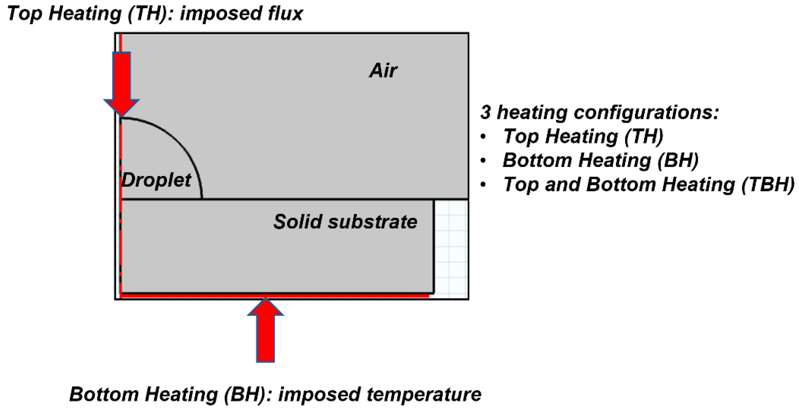
To further analyze and quantify the experimental works proposed in the literature, a comprehensive numerical study was proposed to investigate the influence of the heating regime on Marangoni circulation. We used a comprehensive physical formulation and developed a computational model in COMSOL Multiphysics to simulate the evaporation of a sessile droplet placed on a substrate and surrounded by ambient air. To reach this goal, we considered three different heating configurations. In the first one, the heat was simply supplied from the bottom of the drop support. The second one was inspired by the experimental work proposed in [46]—a heat flux was imposed at the top of the droplet. The third configuration was a combination of both (Figure 1). The balance between the two sources of heat was triggered by the nature (glass and PTFE) and the thickness of the substrate.
2. Mathematical Model
2.1. Physical Domain
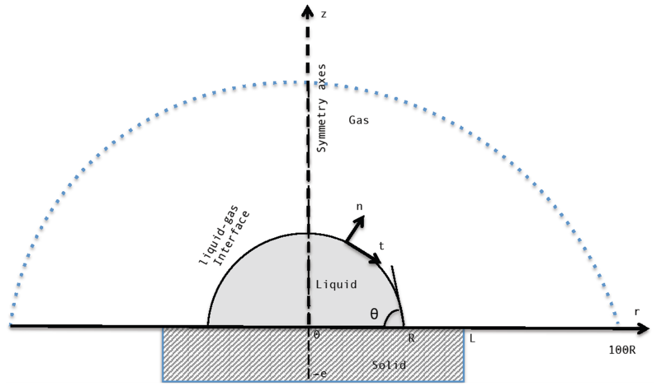
The simulated physical domain is shown in Figure 2. The liquid droplet of radius R, surrounded by air, was placed on a solid substrate. The substrate had a thickness, denoted as ‘e’, and the droplet formed an angle θ with the horizontal plane. In this study, we assumed a 2D geometry with the cylindrical coordinates r and z [20,52,53]. The droplet took the form of a spherical cap during evaporation and it was assumed to be pinned [22,24,25,31].
Viscous shear stresses caused by the outside air on the droplet were neglected. In the fluid zones, the thermophysical properties were assumed to be constant, and the surface tension was assumed to be dependent on the temperature (see Equation (13)).
The droplet size was less than the capillary length (Lc =), so gravity was neglected compared to the surface tension, and thus, the droplet took the form of a spherical cap during evaporation.
The low value of the Bond number (Bo = < 1) confirms that the thermocapillarity dominated the flow inside the droplet compared to the floatability.
2.2. ALE Formulation
In our study, we considered domain 1 (the droplet) that evaporated in domain 2 (the air), presenting a mobile liquid–gas interface. To manage the motion of the interface and the volume of the time-dependent domains, different techniques have been proposed in the literature, such as the Marker and Cell (MAC) method, the volume of fluid (VOF) method, the Level Set method (LS), and the ALE formulation (Arbitrary Lagrangian–Eulerian Method), the latter of which was adopted in this study to model the movement of the liquid–gas interface.
The ALE technique, based on the deformed mesh method [25,54,55], combines the advantages of the Lagrangian and Eulerian methods, allowing for mobile frontiers without moving the mesh. We introduced a third coordinate (linked to the mesh) to this method, and partial differential equations were formulated in the grid coordinate system.
Using the ALE technique, the computation mesh inside of the domains can move arbitrarily to optimize the shapes of the elements. In fact, the mesh nodes can:
- move with the materials (at the interface liquid–gas) to accurately reproduce the moving boundaries and interfaces of multi-domain systems;
- be fixed in space inside the material domain;
- be fixed in one direction and move with the material in other directions.
In the three-coordinate system, one is related to space (x), another is related to the domain (X), and the other is linked to the mesh (Xm) [25,31,56]. Therefore, the velocities are defined as U(X, t) in the area and U(Xm, t) in the mesh, as follows:
The Lagrangian formulation is defined by constant material coordinates, so the material derivative of the spatial coordinate x is
In the ALE formulation,
Combining Equations (3) and (4), we get the convective velocity Uc, as follows:
In the governing equations for droplet evaporation, U(Xm,t) is the flow velocity. In the advection term, the velocity is denoted as Uc. In the rest of the paper, for simple notations, the velocity U(Xm,t) is denoted as U. Consequently, the material derivative of each physical quantity φ is written as follows:
2.3. Governing Equations System
Several physical phenomena were combined in this study: the heat conduction equation in the solid substrate, the continuity (mass conservation), the Navier–Stokes and the energy equations inside the liquid droplet and in the gas phase, and the advection–diffusion equation in the gas phase. Indices l, s, and g used in the equations and in the boundary conditions refer respectively to the liquid, solid, and gas phases. Based on the assumptions considered and the ALE method described above, the equations are written, in the cylindrical coordinates (r,z), as follows [22,25,52]:
- Conduction equation in the solid substrate:
- Continuity, Navier–Stokes, and energy equations in the liquid droplet and gas domain:
- Advection-diffusion equation in the gas domain, with air surrounding the droplet:
- At the liquid–gas interface.
At the interface, the surface tension is a function of the temperature. It is expressed along the interface, its variation causes the Marangoni circulation, it is given by the following equation [52]:
The concentration of the saturated vapor at the droplet surface depends on the interface temperature field. The shape and position of the liquid–gas interface vary with the amount evaporated. The saturated vapor is considered at the liquid–gas interface.
For water, the saturation vapor pressure Pv,sat involving the saturation temperature Tsat is given by the following expression [25]:
The saturation concentration Csat is calculated based on the saturation pressure Pv,sat, such that:
The local evaporated flux is calculated at the liquid–gas interface according to the following equation:
Mw is the molar mass of liquid (water) and D is the diffusion coefficient.
The shape and position of the liquid–gas interface vary with the local evaporated flux mev. The thermal and dynamic conditions at the interface are as follows [25,31,52]:
Equations (17) and (18) respectively describe the balance between the amount of heat transferred by conduction at the interface with the rate of evaporation and the conservation of mass at the free surface, which results in the equality between the amount of fluid moving towards the interface and the amount of evaporated liquid.
2.4. Initial and Boundary Conditions
The fluid phases (air and water) are initially assumed at rest (u = w = 0) and at atmospheric temperature T0 and humidity H0. Initially, the substrate is also at temperature T0.
2.4.1. Boundary Conditions
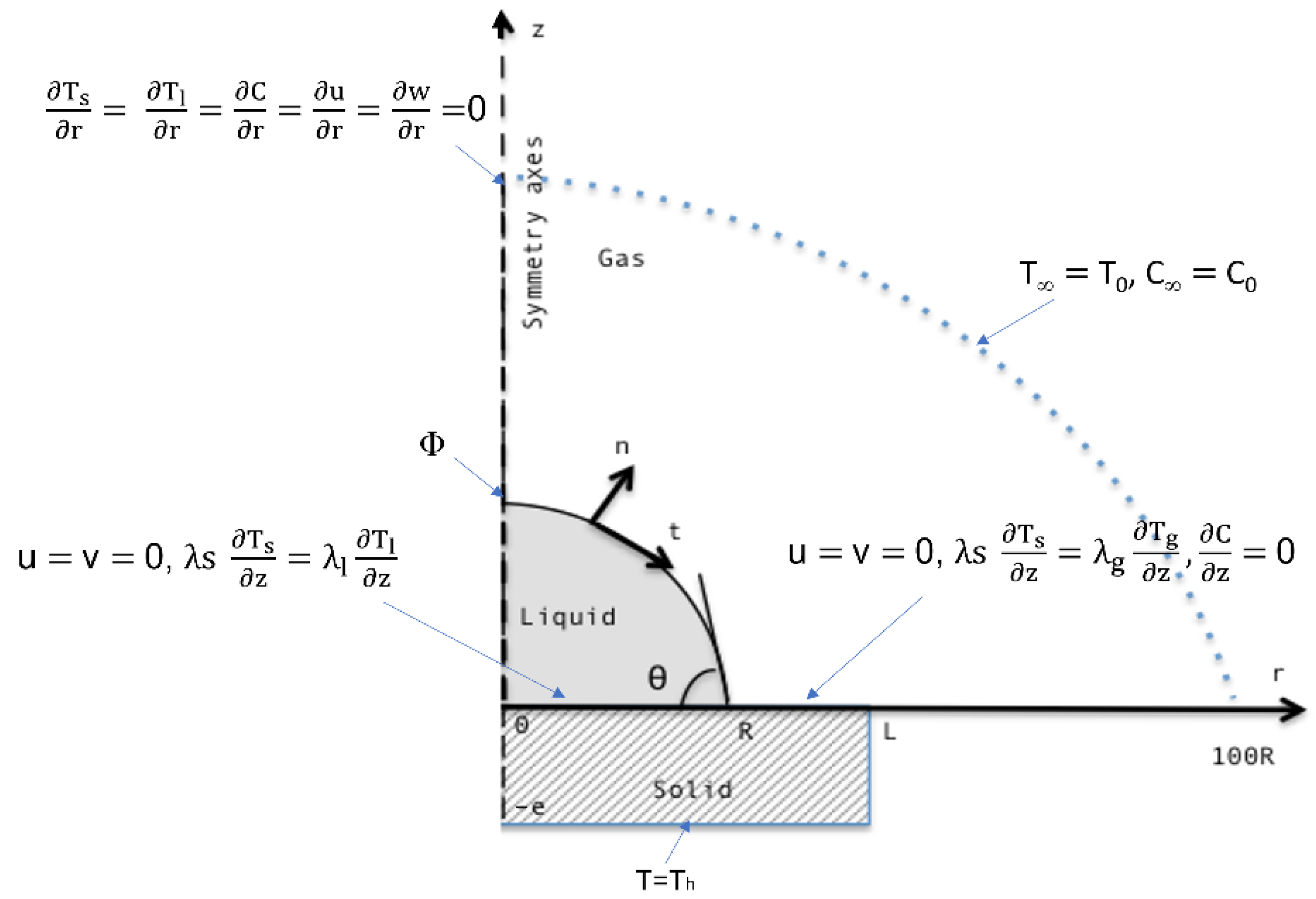
We applied the boundary conditions at the liquid–solid interface, solid–gas interface, symmetry axis, substrate base (heating temperature), top of the droplet (heating flux), and away from the droplet, as follows (Figure 3):
- At r = 0,
- At r = 0, z = h,
- At z = −e,
- At z = 0, 0 < r < R,
- At z = 0, R < r < L,
- At z = ∞,
2.4.2. Heating Configurations
Imposing a temperature value on the substrate is a classic case, widely investigated in the literature. On the other hand, imposing a heating flux on the top of the droplet is not frequent in the literature. Indeed, we found the case of [46], which exposed a laser beam on the top of the droplet.
In this section, we consider three heating configurations: heated substrate or bottom heating (BH) (classical configuration), heated droplet top or top heating (TH), and the combination between the previous two (TBH) (Figure 1). With the three situations, we compare the thermal and dynamic behavior inside the droplet, including the direction of the flow, the evaporated mass, as well as the variation in the temperature.
In the BH configuration, we imposed at the base of the substrate a temperature Th of 50 °C. On the other hand, when dealing with the TH configuration, we imposed at the top of the droplet (on a line of 50 μm) a heating flux Φ of 40 mW. The objective of choosing these boundary conditions was to qualitatively validate our numerical results with the experimental results of [46].
Concerning the TBH configuration, we kept the same value of the imposed temperature (Th = 50 °C) and we decreased the value of the flux (Φ = 3 mW) in order to highlight the two Marangoni circulations.
3. Numerical Simulation
3.1. Mesh Velocity and Balanced Stresses
Two extra equations were added to the thermal and dynamic modeling presented at the interface (Equations (17) and (18)). The first relates to the displacement of the grid and the second defines the stress equilibrium [25,31,52]:
where mev is the local evaporated flux defined by Equation (16), n presents the normal vector of the interface, is the total stress tensor, and fst represents the force per unit area due to the surface tension σ.
where ∇st is the surface gradient operator.
where I is the identity matrix.
The force fst is described by two components, normal and tangential, and we write the balance of the forces as follows:
where rc is the curvature radius and is the tangential vector of the interface.
3.2. Computer Code and Used Grid
The simulation of the evaporation phenomenon of the sessile droplet and the resolution of the system of equations presented with the boundary conditions, as well as the modeling of the displacement of the liquid–gas interface based on the ALE method described previously, were carried out at using the calculation code of the finite element method-based commercial software package COMSOL Multiphysics [25,31,55,56].
Indeed, the monitoring of the mobile interface during the evaporation process is managed by COMSOL’s “mobile mesh” interface. This interface implements the ALE technique for tracking moving boundaries (liquid–gas interface in our case).
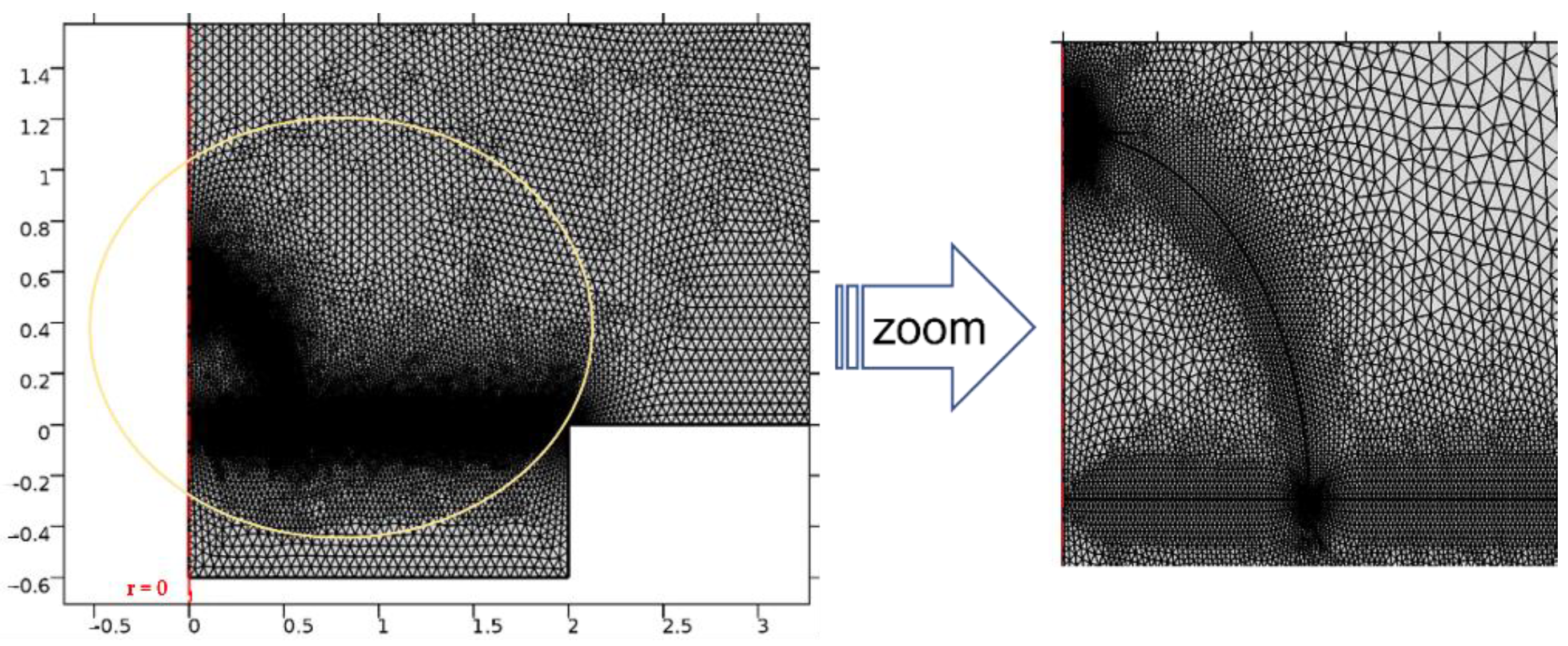
The mesh used for the simulations is shown in Figure 4. It is refined at the interfaces, at the top of the droplet, and at the triple point. The physical domains (air, liquid droplet, and solid substrate) are discretized using triangular elements. The discrete form of all of the PDEs (Equations (7)–(12)) and the boundary conditions (Equations (19)–(28)) yield a nonlinear system of coupled algebraic equations.
In order to make sure of the independence of the results towards a variation of the mesh, we performed a sensitivity analysis test of the mesh size. We considered three different grid sizes. In Table 1, we list the results of the simulation for the different meshes. We considered, at time t = 100 s, the average values of the temperature and the evaporated flow rate at the level of the interface, as well as the volume of the droplet, for the TH, BH, and TBH configurations. The maximum relative difference computed between grids 1 and 2 or grids 2 and 3 is calculated as follows:
where φ = (T, mev,V) and i represents the number of the grid, i = 1,2.
The values in this table show that the simulation results remained stable for the meshes considered. From grid 2 to grid 3, the maximum relative difference did not exceed 0.3% for the TH configuration, 0.45% for the BH configuration, and 1% for TBH. Consequently, in this study, we considered a mesh described by grid 2.
4. Results and Discussion
In Section 4.1, we validate the model and the computer code by comparing the results of the simulation with those of the literature. In Section 4.2, we present the TH and BH configurations (case of one single heat source) and examine their impact on the thermal and dynamic behavior of the evaporated droplet. Section 4.3 presents our study on the influence of the nature and the thickness of the substrate on the thermal and dynamic behavior of the droplet, for the TBH configuration (case of two heat sources). We considered two types—glass and polytetrafluoroethylene (PTFE).
4.1. Model Validation
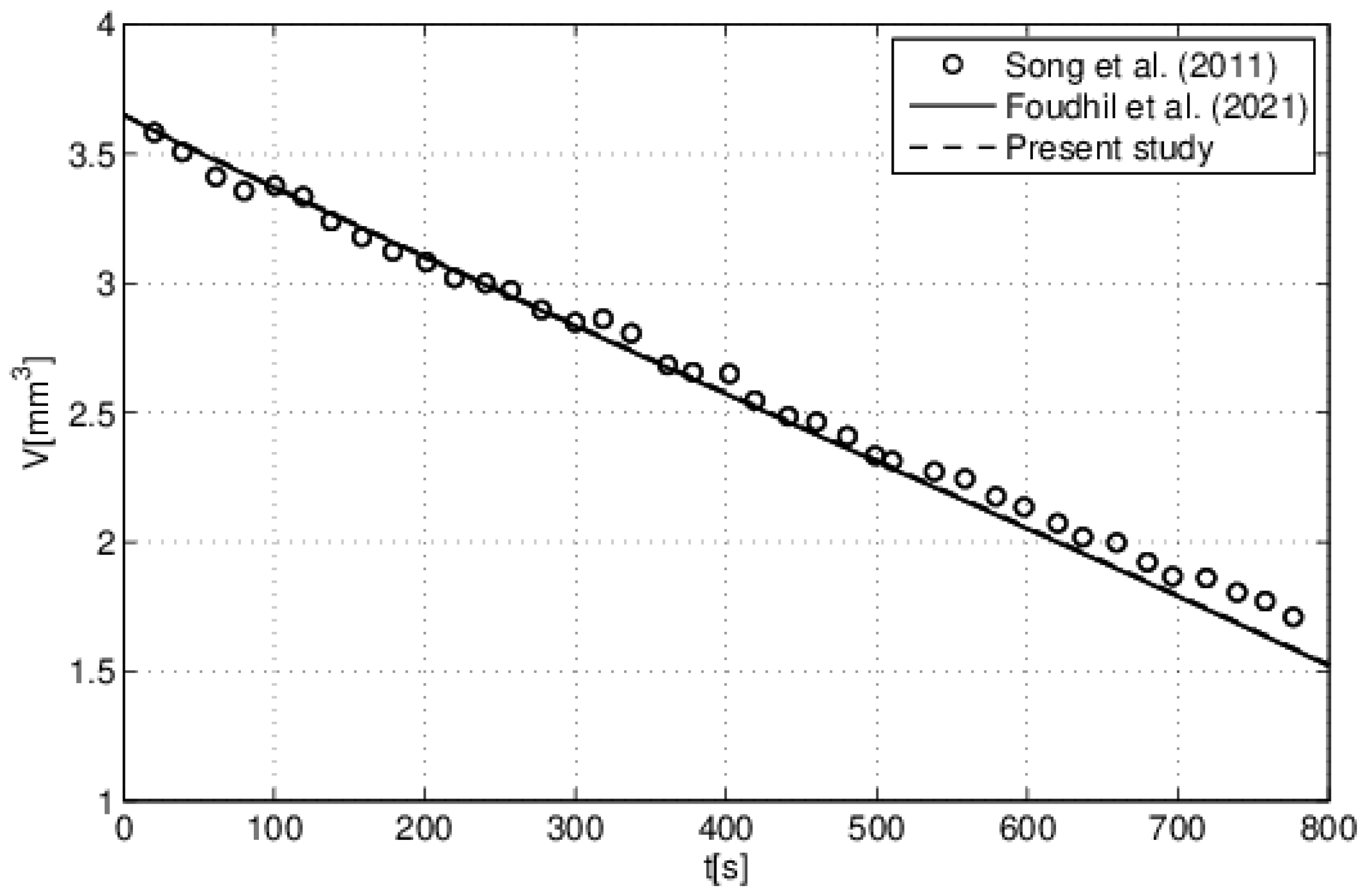
The validation of the mathematical model and the computer code was performed by comparing the results of the simulation with those in the literature. Figure 5 describes the time evolution of the droplet volume in the case of an unheated substrate. The comparison was made with the experimental work presented in [57] and the numerical study in [31].
In the experimental work [57], the authors considered the evaporation of a water droplet with an initial volume equal to 3.64 mm3 and an initial contact angle equal to 57.2°, deposited on a glass substrate. The environment surrounding the droplet (i.e., temperature and humidity) was controlled, and the droplet evaporated under ambient conditions (T = 25 °C and H = 40%). The numerical work in [31] and the present work have reproduced the same experimental conditions presented in [57].
Satisfactory agreement was observed between the results (see Figure 5). The reason for the small scatters could be due to the experimental measurement errors, as well as the pinned mode assumption adopted in our model.
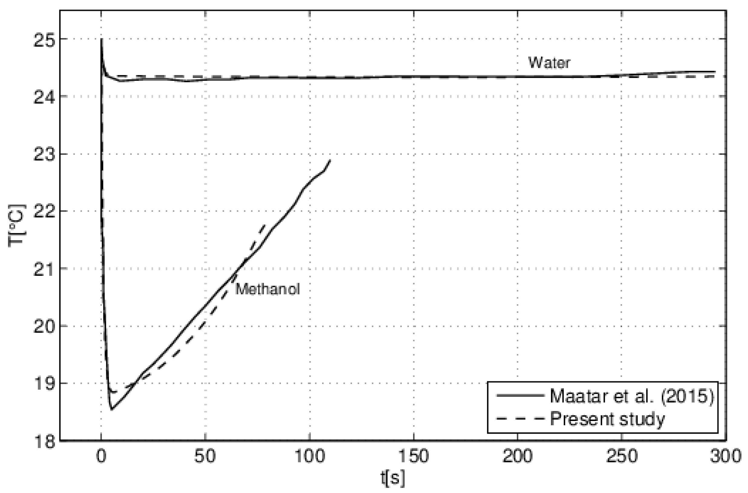
Another comparison is presented in Figure 6 regarding the time evolution of the droplet top temperature considering two different liquids: water and methanol. Indeed, we compared our results with the numerical results of [22], which studied the effect of droplet volatility on the evaporation process. In their study, [22] developed a Fortran computer code based on the finite volume method for solving equations describing the evaporation of a droplet (water or alcohol) deposited on a solid substrate. A satisfactory agreement is observed. In Figure 6, it can be observed the cooling of the droplet following evaporation. Indeed, the phase change by evaporation consumes energy and, therefore, cools the surrounding environment. We also observed that the degree of cooling depends on the nature of the droplet. In fact, the more volatile a droplet is, the more intense its cooling is.
4.2. Marangoni Circulation in the Case of One Single Heat Source (TH and BH Configurations)
In this section, we present our study on the two configurations involving one single source of heat, either from the top through a heat flux or from the bottom through the heated substrate. These simple and contrasted configurations are intended to analyze the main physical phenomena and to depict simple ways to trigger and inverse the Marangoni circulation.
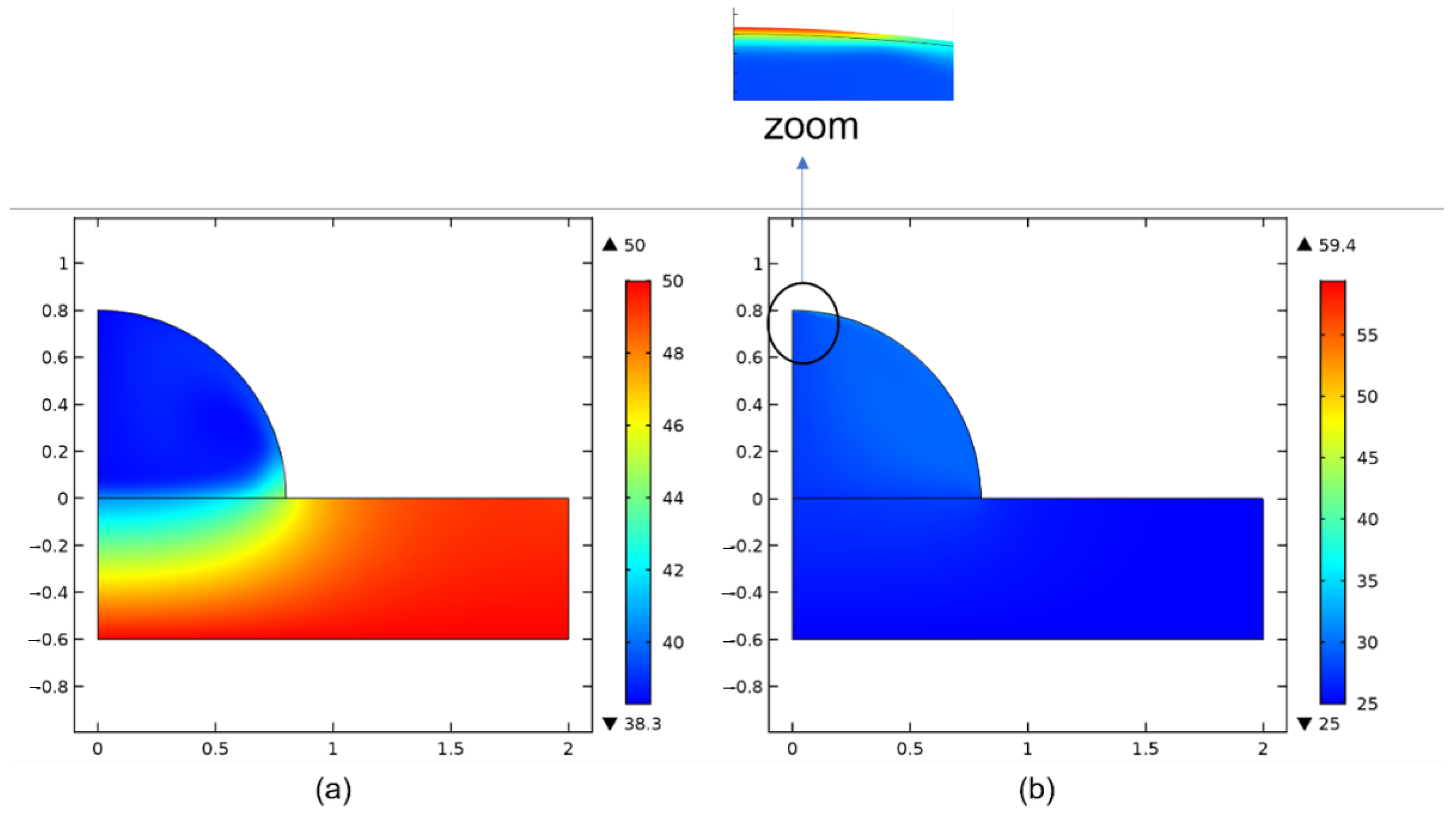
Figure 7 describes the temperature fields in the glass substrate and in the droplet for two different heating configurations (Figure 1): TH (heat flux imposed at the top of the droplet) and BH (temperature imposed at the base of the substrate). From the thermal fields, it can be observed that the TH shows a higher temperature profile at the top of the droplet.
Figure 8 describes the evolution of the temperature field along the liquid–gas interface at time t = 1 s. In this figure, r = 0 mm represents the triple point and r = 1.25 mm, the apex of the droplet. For the classic BH configuration, the temperature variation along the interface did not exceed 7–8 °C (mean value of 40 °C). Regarding the TH configuration, the temperature variation along the interface did not exceed 2 °C for over 80% of its length (average value close to 30 °C), then, approaching the top of the droplet, the temperature rise to 60 °C.
For the studied configurations, it was important to know the distribution of the temperature in the droplet, especially at the interface. Indeed, surface tension is a function of the temperature (see Equation (13)), and its variation is the driving force for the Marangoni circulation.
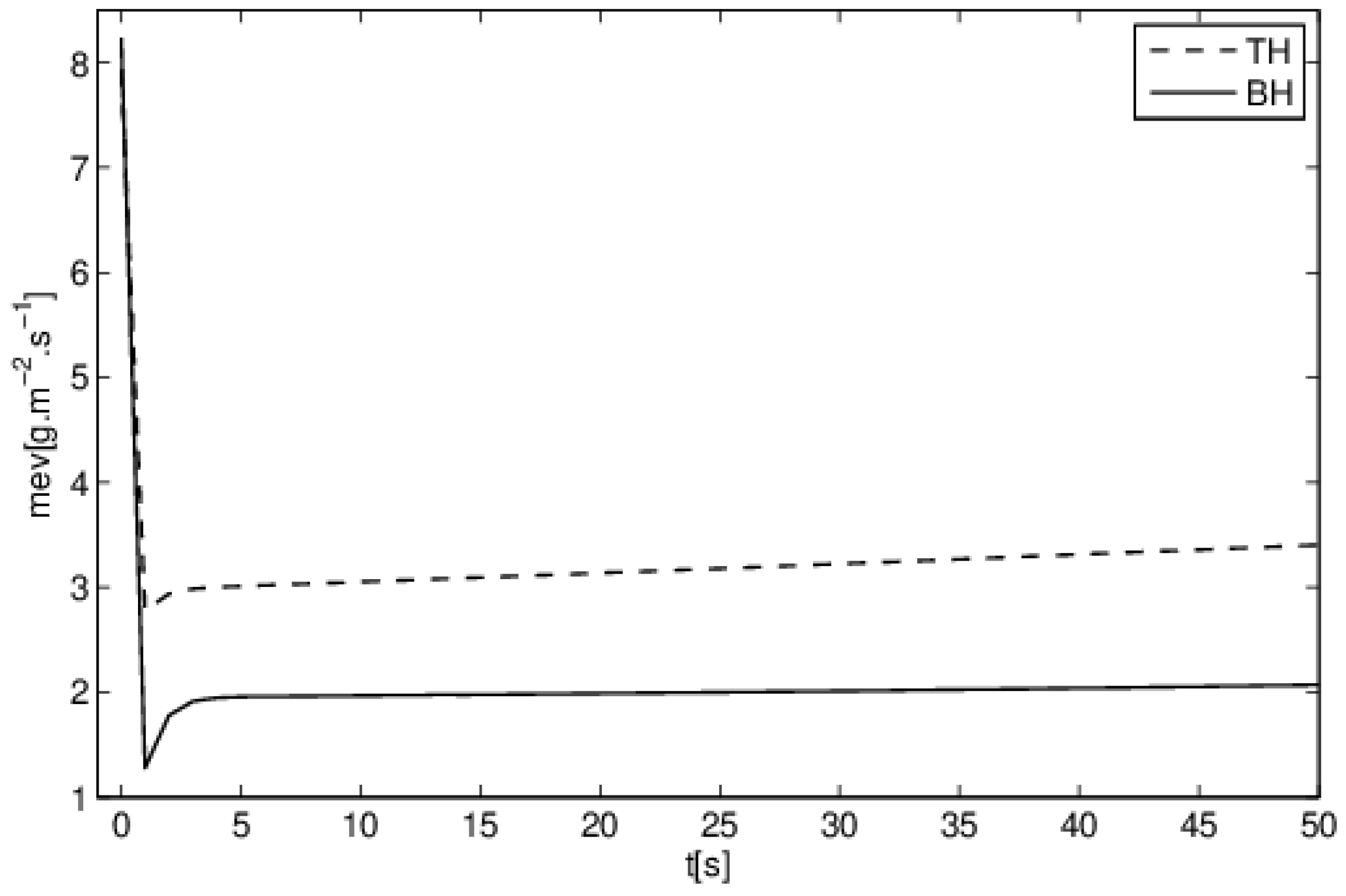
In Figure 9, we represent the temporal evolution of the average evaporated flux for the two studied configurations TH and BH. The evaporated flux presents the maximum values at the first moments, and then it evolves towards quasi-constant values. Indeed, at the beginning of evaporation, the concentration gradient is important, as it promotes evaporation, and then the air is enriched in vapor, and the values of the evaporated flow rate decrease.
These curves show that the average flux rate was important for the TH configuration, which had a very high local density near the top of the droplet. Overall, the evaporation rate was higher for the case of the BH configuration, since the average temperature was higher for this configuration (Figure 7 and Figure 8), which accelerated the evaporation of the droplet.
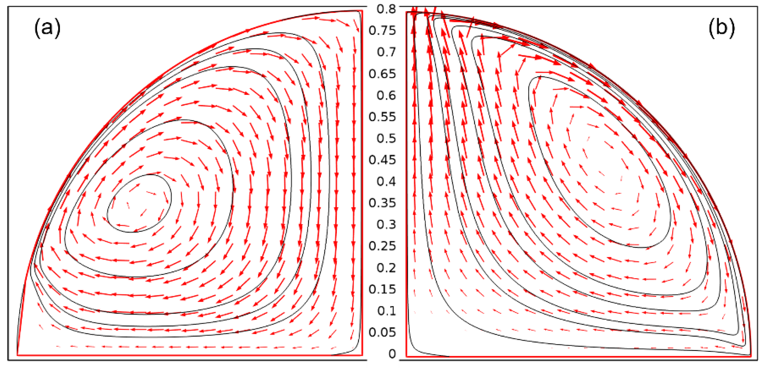
Figure 10 describes the direction of the flow in the droplet for the two configurations TH and BH. As Marangoni circulation is driven by the effect of temperature on the surface tension, it consistently obtained an inverted circulation between the two configurations.
When the heat came from the substrate (BH), the surface tension had low values at the contact line (high temperature) and high values at the top of the droplet (low temperature), and an upward movement of the fluid was observed along the droplet interface (Figure 10a). The water evaporation flux was highest at the edge of the droplets, so an internal flux had to be provided to replenish the water loss at the edge. As a consequence of this Marangoni circulation and in the case of droplets containing particles, radial outward flow carried the particles to the edge of the drop, causing the coffee ring effect.
The opposite case is observed in Figure 10b. Due to the variation in the surface tension, which had low values at the top of the droplet (high temperature) and high values at the triple point (low temperature), a downward motion of the fluid along the droplet interface was observed. Due to the heat flux imposed at the top of the droplets, the evaporation flux of the water was highest at the top of the droplet. An internal flow developed to replenish the volume of water lost at the top, producing a radial flow inward (center of the droplets) and reversing/avoiding the coffee ring effect.
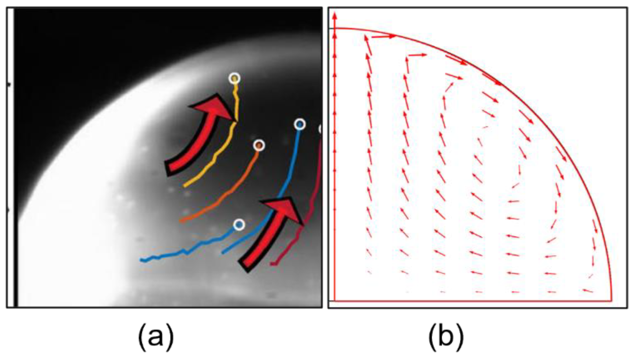
This result confirms the experimental work presented in [46], where a laser beam was applied to the top of a droplet deposited on an unheated substrate. Figure 11 presents a qualitative comparison between the experimental results of [46] and our simulation, showing the reversal of the coffee ring effect.
Moreover, in [46], the authors imposed a laser beam (40 mW) at the top of the droplet, which accelerated its evaporation compared to the case of a heated substrate (50 °C). This was not the case in our simulation since we imposed a flux at the top of the droplet. Indeed, the laser beam did not just heat the top of the droplet but crossed it and heated the entire droplet, which was not the case in our study.
4.3. TBH Configuration and Nature Substrate Effect
In this section, we present our study on the TBH configuration (see Figure 1), in which two sources of heat coexisted: the top flux and the heated bottom plate. In order to change the balance between the top and bottom fluxes, the heat flux supplied by the substrate was changed by the type of substrate and its thickness. We considered two types of substrates (see Table 2)—glass and polytetrafluoroethylene (PTFE).
4.3.1. Marangoni Circulation
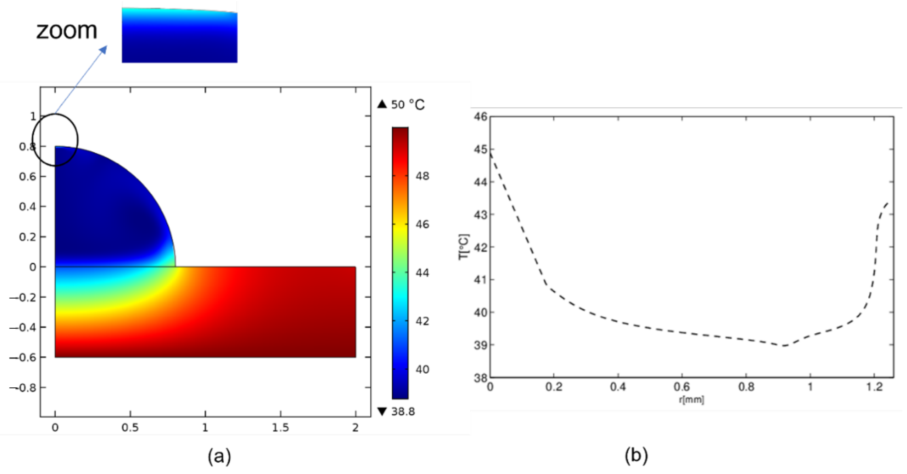
Figure 12a describes the temperature field in the droplet and in the substrate when a flux was imposed at the top of the droplet at the order of 3 mW and a temperature at the base of the substrate equal to 50 °C. Moving from the triple point, r = 0 mm, towards the top of the droplet, r = 1.25 mm, the temperature values along the interface decreased (temperature imposed on the substrate). Then, at a given position, these values increased (flux imposed on the top of the droplet). This non-homogeneity of the temperature along the interface (Figure 12b) resulted in non-homogeneity of the surface tension (which depended on the temperature). This double variation of the surface tension generated a double variation of the Marangoni circulation manifested by two vortices, describing an upward and downward flow along the interface (see Figure 13).
4.3.2. Substrate Type Effect
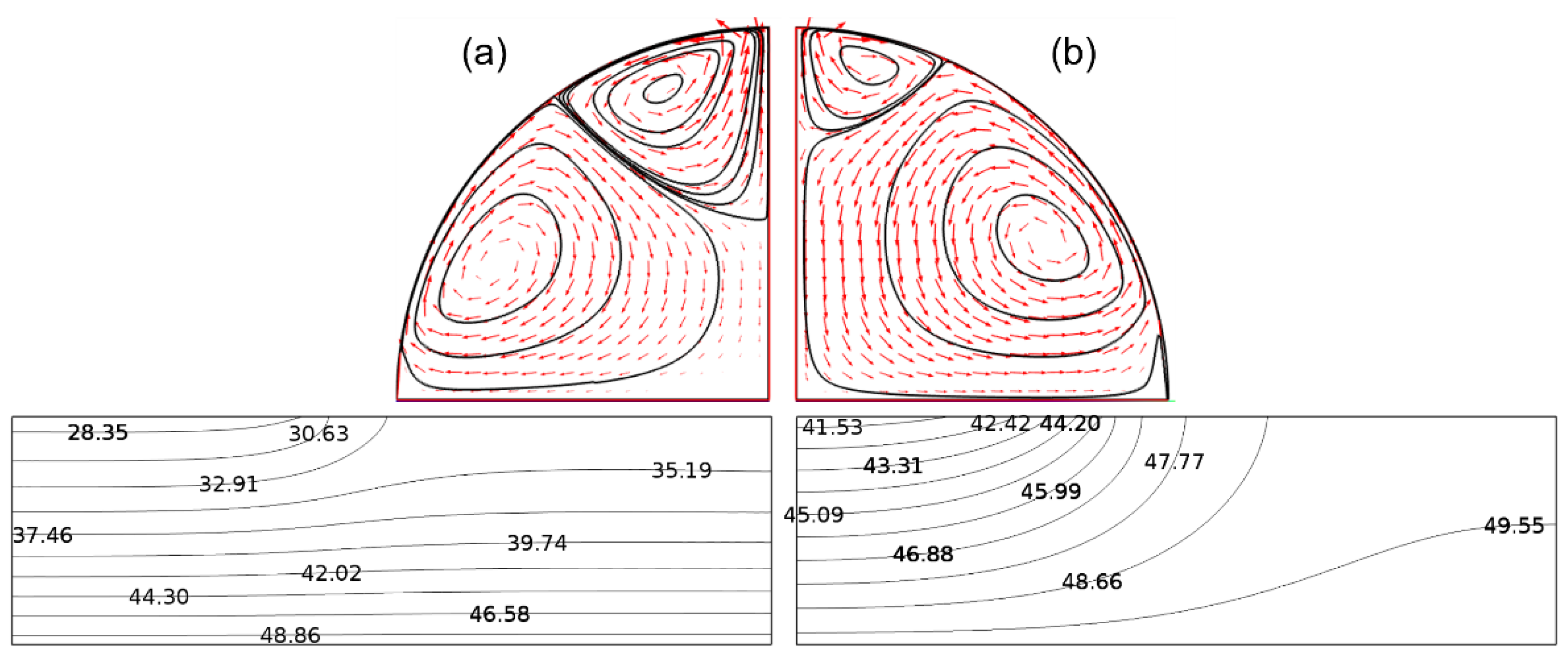
Figure 13 describes the direction of flow in the droplet for the TBH configuration and for the two types of substrates used—glass and PTFE (see Table 2).
In both cases, the global trend was the appearance of two vortices in the droplet. The first was an upward Marangoni flow along the interface, and the second was a downward Marangoni flow. Indeed, this double behavior was linked to the two thermal conditions used—a temperature imposed on the substrate (upward flow) and a flux imposed on the top of the droplet (a downward flow).
However, the effect of the type of substrate, due to its thermal conductivity, changed the conductive flux through its thickness, and hence, the intensity of the heat supplied to the droplet from the bottom.
The isotherms in the substrate, as plotted in Figure 13, also proved that, in the case of the glass, the most conductive substrate, a lateral thermal gradient also drove heat radially. Compared to the PTFE, the temperatures in the case of the glass were consistently higher at the liquid–solid interface: 44.2 °C for the glass versus 30.63 °C for the PTFE. Thus, the use of PTFE reduced the transfer of heat to the substrate and, therefore, to the droplet, which affected the partition of the two vortices. Compared to the case of the glass substrate, the size of the upward vortex was, therefore, reduced.
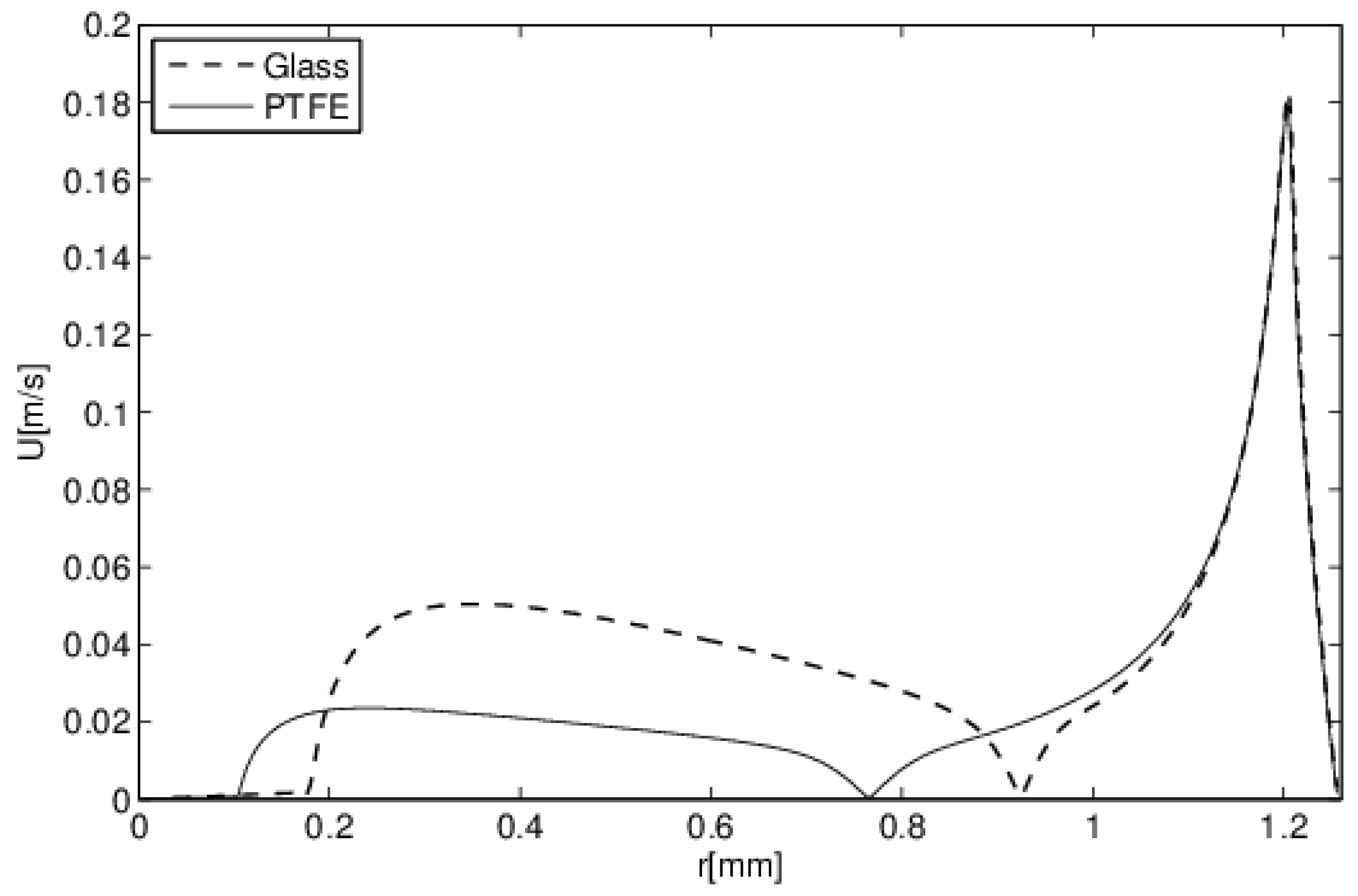
Figure 14 presents the evolution of the flow velocity along the interface for the TBH configuration and for the two types of substrates used, glass and PTFE. These curves show that along the interface, the flow velocity presents two maximum values (of different intensities) separated by a stagnation point (velocity equal to zero). The first increase in the velocity value was related to the upward Marangoni flow circulation, which occurred near the triple point. As explained above, the intensity of the velocity in this zone and its location depended on the nature of the substrate. The second velocity peak occurred near the top of the droplet exposed to a heat flux applied to the top. This peak did not depend on the substrate since it was directly related to the heat flux supplied at the top of the droplet.
4.3.3. Effect of the Substrate Thickness
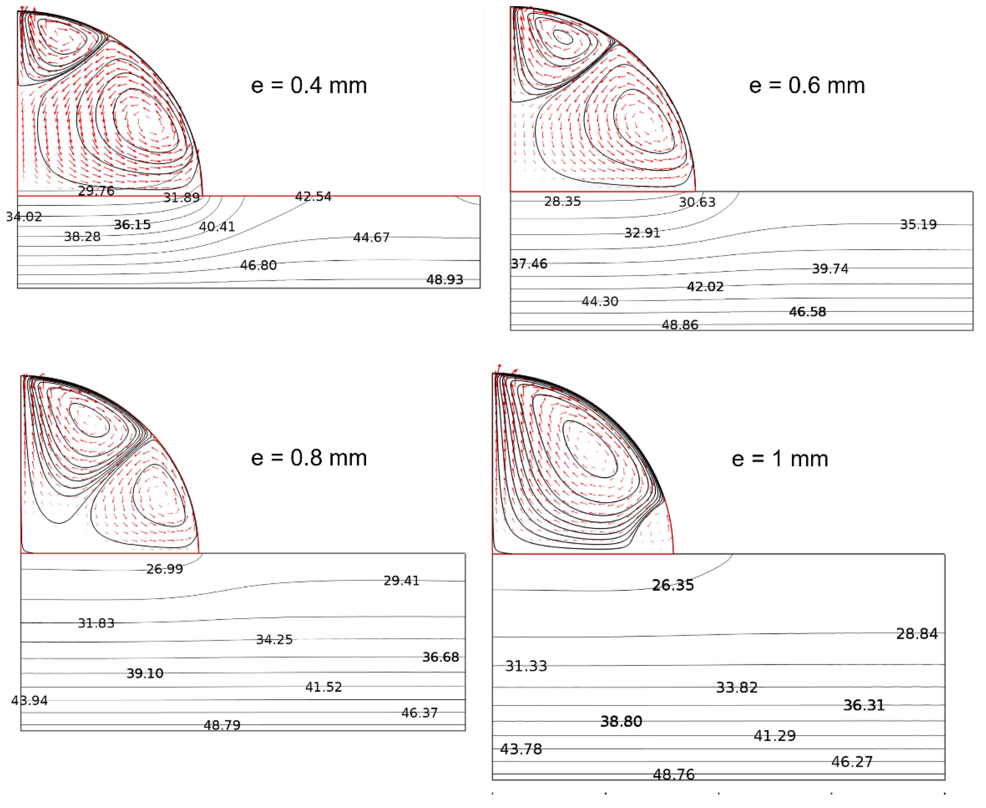
In Figure 15, we present the velocity fields and the Marangoni circulation at the beginning of the evaporation (t = 1 s) for different thicknesses of the PTFE substrate (from 0.4 to 1 mm). The thickness is another way to change the bottom flux supplied to the droplet. Figure 15 confirms that the size of the top vortex increased with the increasing substrate thickness. Obviously, the increase in the substrate thickness reduced the conductive flux, which, in turn, influenced the velocity field and sizes of the vortices.
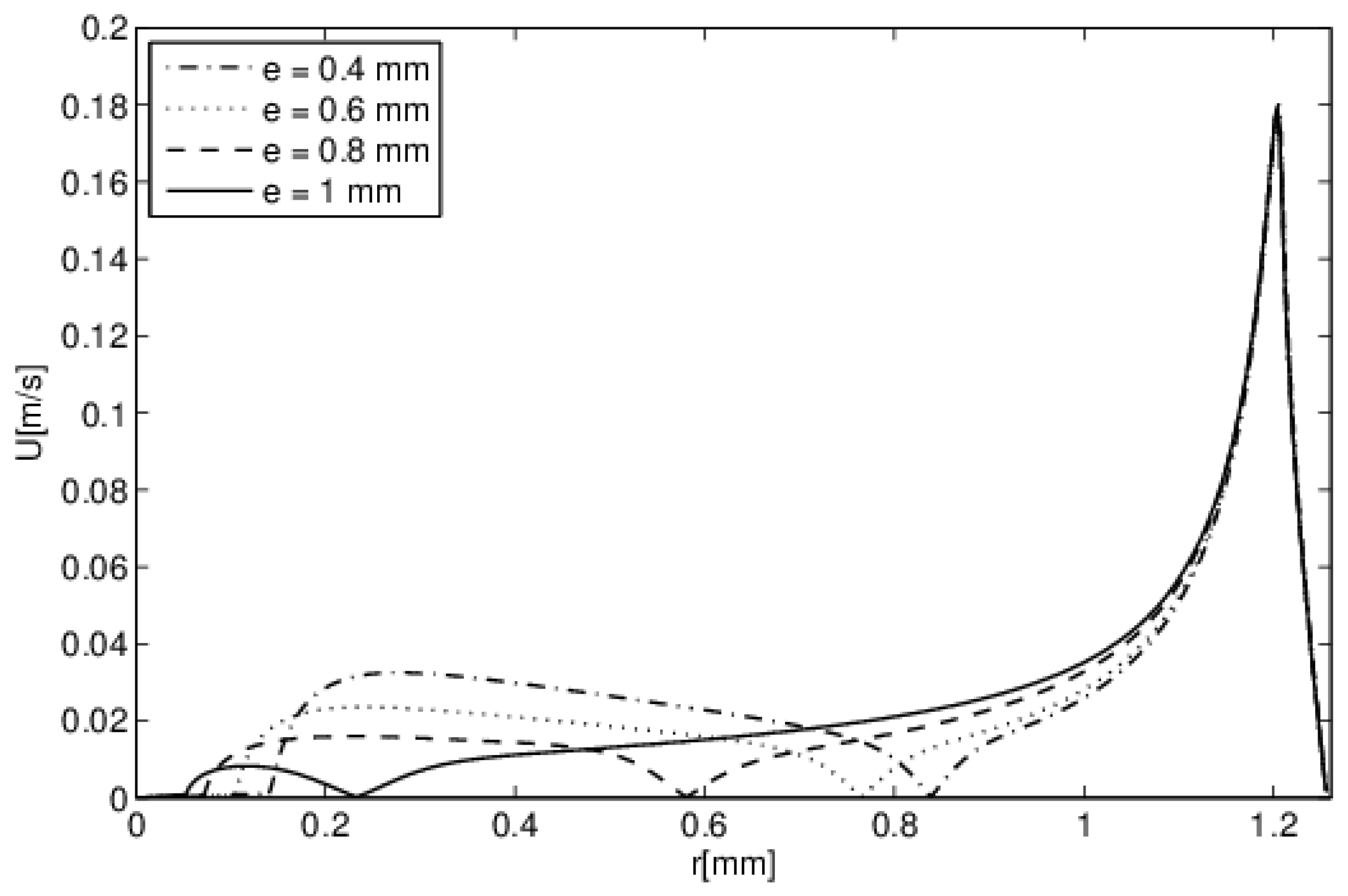
As mentioned before, the two vortices were separated by a stagnation zone. Figure 16 presents the evolution of the velocity of the flow along the interface at the beginning of the evaporation (t = 1 s) for the various thicknesses of PTFE considered. By increasing the thickness of the substrate, the stagnation zone approached the triple point (r = 0 mm). This result confirms the observations in Figure 15.
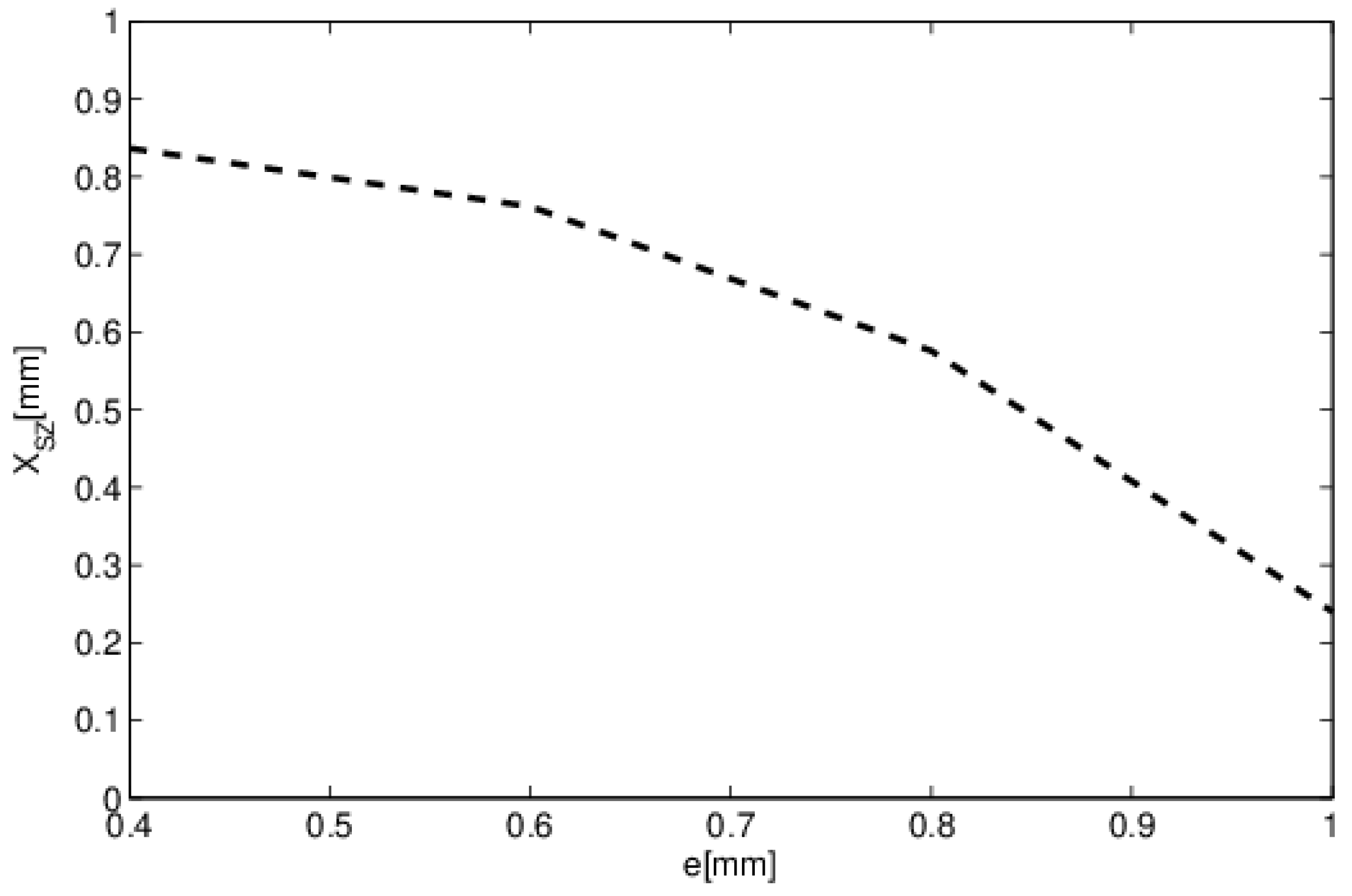
In Table 3, we list the evolution of the stagnation zone with the substrate thickness. The increase in the thickness of the substrate shifted the stagnation zone towards the triple point. These results are depicted in Figure 17, showing the nonlinear approach of the stagnation zone XSZ to the triple point as the thickness of the substrate increased.
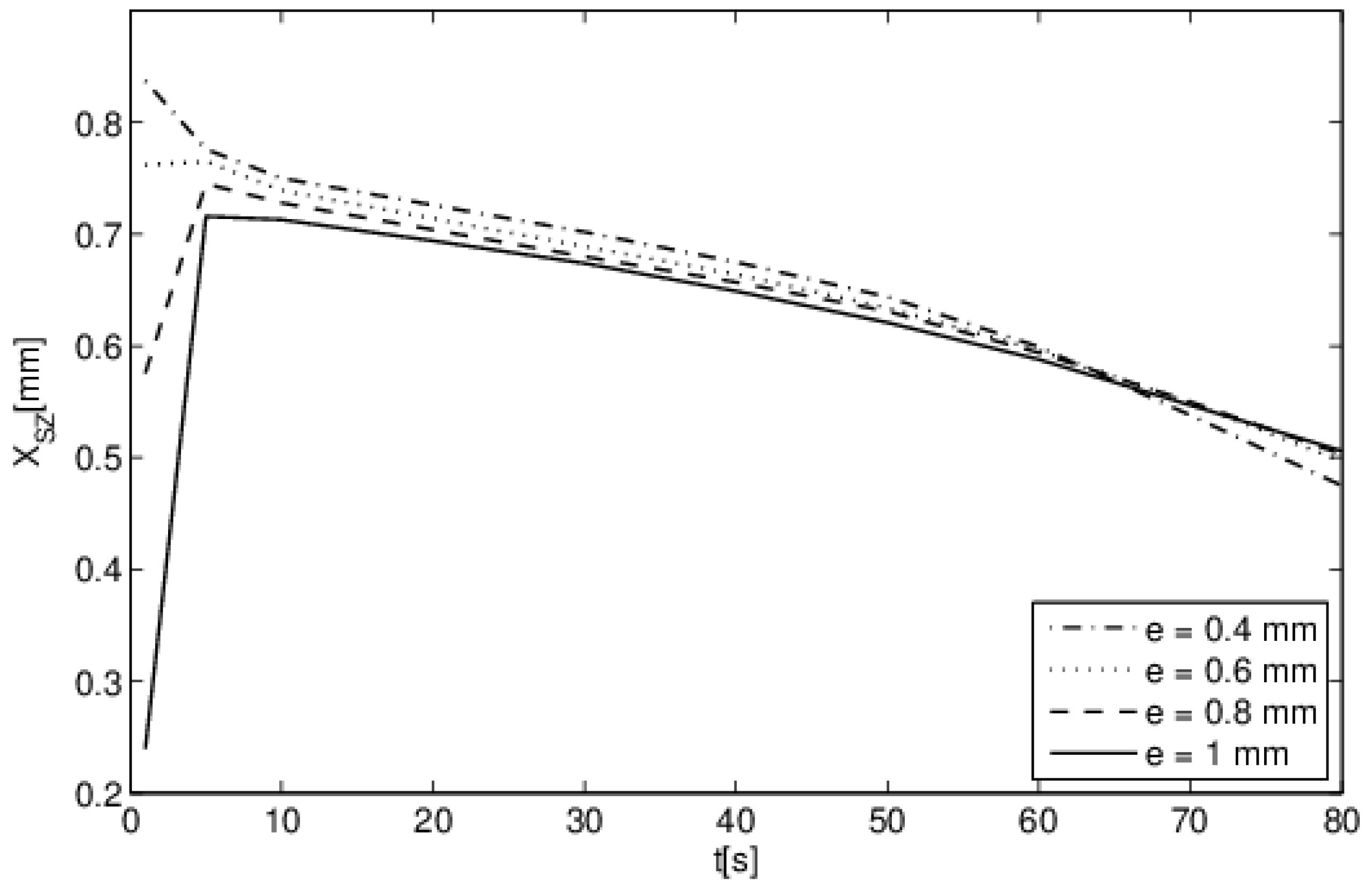
Figure 18 depicts the time evolution of the stagnation zone XSZ for different thicknesses of PTFE substrates. At the start of evaporation (t = 1 s), this zone approached the top of the droplet for small substrate thicknesses, which favored the upward Marangoni flow, and the opposite case was observed when the thickness was large. After t = 10 s, and when the heat propagated towards the liquid–solid interface, the position of the stagnation zone XZS was almost similar to all the thicknesses considered.
5. Conclusions
In this study, we used a comprehensive physical formulation and developed a numerical code to investigate the heat regime on the Marangoni circulation of a droplet evaporating on a substrate. The model considers a sessile liquid droplet deposited on a substrate and surrounded by ambient air. This droplet was subjected to three different heating configurations—heated substrate (BH), droplet top heated (TH), and a combination of both (TBH). The results obtained allow us to draw the following conclusions:
- Using one single source of heat, the direction of Marangoni circulation is monotonic and can be chosen; upward flow occurs when the substrate is heated (BH) and a downward flow occurs when heat is supplied at the top of the droplet (TH);
- The combination of the two types of heating (TBH) triggered a Marangoni flow with two vortices separated by a stagnation point;
- The balance between the magnitude of the two heat sources was changed by the nature and the thickness of the substrate. The results show that the respective importance of the two vortices and the position of the stagnation point can be controlled.
This computational study highlights the effect of a double heat source on Marangoni circulation and proves that the Marangoni circulation inside the droplet can be controlled by the heating regime. These results can be exploited to orient the formation of a deposit during the evaporation of droplets containing dissolved components or microparticles, which has an important impact on several industrial aspects.
Author Contributions
Conceptualization, W.F. and S.B.J.; methodology, W.F., C.A., P.P. and S.B.J.; software, P.P.; validation, W.F.; formal analysis, W.F. and C.A.; investigation, W.F. and S.B.J.; writing—original draft preparation, W.F., C.A., P.P. and S.B.J.; writing—review and editing, W.F., C.A., P.P. and S.B.J.; supervision, C.A., P.P. and S.B.J. All authors have read and agreed to the published version of the manuscript.
Funding
This research received no external funding.
Institutional Review Board Statement
Not applicable.
Informed Consent Statement
Not applicable.
Data Availability Statement
Not applicable.
Conflicts of Interest
The authors declare no conflict of interest.
Nomenclature
| Symbols | Abbreviation |
| ALE | Arbitrary Lagrangian–Eulerian (-) |
| BH | Bottom Heating (-) |
| Bo | Bond number (-) |
| C | concentration (mol·L−1 or g·L−1) |
| Cp | heat capacity (J·kg−1·K−1) |
| D | diffusion coefficient (m2·s−1) |
| e | substrate thickness (m) |
| fst | force per unit area (N·m−2) |
| g | gravity acceleration (m·s−2) |
| h | droplet height (m) |
| H | humidity (%) |
| L | substrate length (m) |
| Lc | capillary length (m) |
| Lv | latent heat (J·kg−1) |
| mev | local evaporation rate (kg·m−2·s−1) |
| Mw | molar Mass (kg·mol−1) |
| n | normal direction (-) |
| p | pressure (Pa) |
| rc | curvature radius (m) |
| R | contact radius (m) |
| Rm | universal gas constant (J·mol−1·K−1) |
| (r,z) | cylindrical coordinates (m) |
| SZ | Stagnation zone (-) |
| t | time (s) |
| tangential direction (-) | |
| T | temperature (K or °C) |
| TH | Top Heating (-) |
| TBH | Top and Bottom Heating (-) |
| (u,w) | velocity components (m·s−1) |
| U | norm of velocity (m·s−1) |
| V | droplet volume (mm3 or µL) |
| x | space coordinates (m) |
| X | domain coordinates (m) |
| Xm | mesh coordinates (m) |
| Greek symbols | |
| ε | relative difference (%) |
| θ | contact angle (°) |
| λ | thermal conductivity (W·m−1·K−1) |
| μ | dynamic viscosity (Pa·s) |
| ρ | density (kg·m−3) |
| σ | surface tension (N·m−1) |
| τ | total stress tensor (-) |
| Φ | heat flux (W) |
| Subscripts | |
| c | convective |
| g | gas (air) |
| h | hot |
| l | liquid (water) |
| ∝ | infinite |
| 0 | ambient, reference |
| s | solid (substrate) |
| sat | saturation |
References
- Leenaars, A.F.M.; Huethorst, J.A.M.; Van Oekel, J.J. Marangoni drying: A new extremely clean drying process. Langmuir 1990, 6, 1701–1703. [Google Scholar] [CrossRef]
- Kim, J. Spray cooling heat transfer: The state of the art. Int. J. Heat Fluid Flow 2007, 28, 753–767. [Google Scholar] [CrossRef]
- Park, J.; Moon, J. Control of Colloidal Particle Deposit Patterns within Picoliter Droplets Ejected by Ink-Jet Printing. Langmuir 2006, 22, 3506–3513. [Google Scholar] [CrossRef] [PubMed]
- Wu, L.; Dong, Z.; Kuang, M.; Li, Y.; Li, F.; Jiang, L.; Song, Y. Printing Patterned Fine 3D Structures by Manipulating the Three Phase Contact Line. Adv. Funct. Mater. 2015, 25, 2237–2242. [Google Scholar] [CrossRef]
- MacBeath, G.; Schreiber, S.L. Printing Proteins as Microarrays for High-Throughput Function Determination. Science 2000, 289, 1760–1763. [Google Scholar] [CrossRef]
- Dugas, V.; Broutin, A.J.; Souteyrand, E. Droplet Evaporation Study Applied to DNA Chip Manufacturing. Langmuir 2005, 21, 9130–9136. [Google Scholar] [CrossRef]
- Sempels, W.; De Dier, R.; Mizuno, H.; Hofkens, J.; Vermant, J. Auto-production of biosurfactants reverses the coffee ring effect in a bacterial system. Nat. Commun. 2013, 4, 1757. [Google Scholar] [CrossRef] [Green Version]
- Liu, H. Science and Engineering of Droplets—Fundamentals and Applications; Noyes Publications: Norwich, CT, USA, 2000. [Google Scholar]
- de Gennes, P.-G.; Brochard-Wyart, F.; Quere, D. Capillarity and Wetting Phenomena: Drops, Bubbles, Pearls, Waves; 2004th ed.; Springer: New York, NY, USA, 2013. [Google Scholar]
- Sirignano, W.A. Fluid Dynamics and Transport of Droplets and Sprays, 2nd ed; Cambridge University Press: Cambridge, UK, 2014. [Google Scholar]
- Brutin, D. (Ed.) Droplet Wetting and Evaporation: From Pure to Complex Fluids; Academic Press: San Diego, CA, USA, 2015. [Google Scholar]
- Murisic, N.; Kondic, L. On evaporation of sessile drops with moving contact lines. J. Fluid Mech. 2011, 679, 219–246. [Google Scholar] [CrossRef]
- Picknett, R.; Bexon, R. The evaporation of sessile or pendant drops in still air. J. Colloid Interface Sci. 1977, 61, 336–350. [Google Scholar] [CrossRef]
- Rowan, S.M.; Newton, M.I.; McHale, G. Evaporation of Microdroplets and the Wetting of Solid Surfaces. J. Phys. Chem. 1995, 99, 13268–13271. [Google Scholar] [CrossRef]
- Deegan, R.; Bakajin, O.; Dupont, T.F.; Huber, G.; Nagel, S.R.; Witten, T.A. Contact line deposits in an evaporating drop. Phys. Rev. E 2000, 62, 756–765. [Google Scholar] [CrossRef] [PubMed] [Green Version]
- Hu, H.; Larson, R.G. Evaporation of a Sessile Droplet on a Substrate. J. Phys. Chem. B 2002, 106, 1334–1344. [Google Scholar] [CrossRef]
- Erbil, H.Y. Evaporation of pure liquid sessile and spherical suspended drops: A review. Adv. Colloid Interface Sci. 2012, 170, 67–86. [Google Scholar] [CrossRef]
- Gelderblom, H.; Bloemen, O.; Snoeijer, J.H. Stokes flow near the contact line of an evaporating drop. J. Fluid Mech. 2012, 709, 69–84. [Google Scholar] [CrossRef] [Green Version]
- David, S.; Sefiane, K.; Tadrist, L. Experimental investigation of the effect of thermal properties of the substrate in the wetting and evaporation of sessile drops. Colloids Surf. A Physicochem. Eng. Asp. 2007, 298, 108–114. [Google Scholar] [CrossRef]
- Lu, G.; Duan, Y.-Y.; Wang, X.-D.; Lee, D.-J. Internal flow in evaporating droplet on heated solid surface. Int. J. Heat Mass Transf. 2011, 54, 4437–4447. [Google Scholar] [CrossRef]
- Lopes, M.C.; Bonaccurso, E.; Gambaryan-Roisman, T.; Stephan, P. Influence of the substrate thermal properties on sessile droplet evaporation: Effect of transient heat transport. Colloids Surfaces A Physicochem. Eng. Asp. 2013, 432, 64–70. [Google Scholar] [CrossRef]
- Maatar, A.; Chikh, S.; Saada, M.A.; Tadrist, L. Transient effects on sessile droplet evaporation of volatile liquids. Int. J. Heat Mass Transf. 2015, 86, 212–220. [Google Scholar] [CrossRef]
- Khilifi, D.; Foudhil, W.; Harmand, S.; Ben Jabrallah, S. Evaporation of a sessile oil drop in the Wenzel-like regime. Int. J. Therm. Sci. 2020, 151, 106236. [Google Scholar] [CrossRef]
- Saada, M.A.; Chikh, S.; Tadrist, L. Numerical investigation of heat and mass transfer of an evaporating sessile drop on a horizontal surface. Phys. Fluids 2010, 22, 112115. [Google Scholar] [CrossRef]
- Yang, K.; Hong, F.; Cheng, P. A fully coupled numerical simulation of sessile droplet evaporation using Arbitrary Lagrangian–Eulerian formulation. Int. J. Heat Mass Transf. 2013, 70, 409–420. [Google Scholar] [CrossRef]
- Askounis, A.; Sefiane, K.; Koutsos, V.; Shanahan, M.E. Effect of particle geometry on triple line motion of nano-fluid drops and deposit nano-structuring. Adv. Colloid Interface Sci. 2015, 222, 44–57. [Google Scholar] [CrossRef] [PubMed]
- Girard, F.; Antoni, M.; Faure, S.; Steinchen, A. Influence of heating temperature and relative humidity in the evaporation of pinned droplets. Colloids Surfaces A Physicochem. Eng. Asp. 2008, 323, 36–49. [Google Scholar] [CrossRef]
- Diddens, C. Detailed finite element method modeling of evaporating multi-component droplets. J. Comput. Phys. 2017, 340, 670–687. [Google Scholar] [CrossRef]
- Diddens, C.; Tan, H.; Lv, P.; Versluis, M.; Kuerten, J.G.M.; Zhang, X.; Lohse, D. Evaporating pure, binary and ternary droplets: Thermal effects and axial symmetry breaking. J. Fluid Mech. 2017, 823, 470–497. [Google Scholar] [CrossRef] [Green Version]
- Diddens, C.; Kuerten, J.; van der Geld, C.; Wijshoff, H. Modeling the evaporation of sessile multi-component droplets. J. Colloid Interface Sci. 2017, 487, 426–436. [Google Scholar] [CrossRef]
- Foudhil, W.; Chen, P.; Fahem, K.; Harmand, S.; Ben Jabrallah, S. Study of the evaporation kinetics of pure and binary droplets: Volatility effect. Heat Mass Transf. 2021, 57, 1773–1790. [Google Scholar] [CrossRef]
- Hu, H.; Larson, R.G. Analysis of the Microfluid Flow in an Evaporating Sessile Droplet. Langmuir 2005, 21, 3963–3971. [Google Scholar] [CrossRef]
- Ristenpart, W.D.; Kim, P.G.; Domingues, C.; Wan, J.; Stone, H.A. Influence of Substrate Conductivity on Circulation Reversal in Evaporating Drops. Phys. Rev. Lett. 2007, 99, 234502. [Google Scholar] [CrossRef] [Green Version]
- Xu, X.; Luo, J.; Guo, D. Criterion for Reversal of Thermal Marangoni Flow in Drying Drops. Langmuir 2009, 26, 1918–1922. [Google Scholar] [CrossRef]
- Shi, W.-Y.; Tang, K.-Y.; Ma, J.-N.; Jia, Y.-W.; Li, H.-M.; Feng, L. Marangoni convection instability in a sessile droplet with low volatility on heated substrate. Int. J. Therm. Sci. 2017, 117, 274–286. [Google Scholar] [CrossRef]
- Tan, H.; Diddens, C.; Lv, P.; Kuerten, J.G.M.; Zhang, X.; Lohse, D. Evaporation-triggered microdroplet nucleation and the four life phases of an evaporating Ouzo drop. Proc. Natl. Acad. Sci. USA 2016, 113, 8642–8647. [Google Scholar] [CrossRef] [PubMed] [Green Version]
- Karapetsas, G.; Sahu, K.C.; Matar, O.K. Evaporation of Sessile Droplets Laden with Particles and Insoluble Surfactants. Langmuir 2016, 32, 6871–6881. [Google Scholar] [CrossRef] [PubMed]
- Deegan, R.D.; Bakajin, O.; Dupont, T.F.; Huber, G.; Nagel, S.R.; Witten, T.A. Capillary flow as the cause of ring stains from dried liquid drops. Nature 1997, 389, 827–829. [Google Scholar] [CrossRef]
- Mampallil, D.; Eral, H.B. A review on suppression and utilization of the coffee-ring effect. Adv. Colloid Interface Sci. 2018, 252, 38–54. [Google Scholar] [CrossRef] [PubMed]
- Hu, A.H.; Larson, R.G. Marangoni Effect Reverses Coffee-Ring Depositions. J. Phys. Chem. B 2006, 110, 7090–7094. [Google Scholar] [CrossRef]
- Zhang, Z.; Zhang, X.; Xin, Z.; Deng, M.; Wen, Y.; Song, Y. Controlled Inkjetting of a Conductive Pattern of Silver Nanoparticles Based on the Coffee-Ring Effect. Adv. Mater. 2013, 25, 6714–6718. [Google Scholar] [CrossRef]
- Lee, K.-H.; Kim, S.-M.; Jeong, H.; Jung, G.-Y. Spontaneous nanoscale polymer solution patterning using solvent evaporation driven double-dewetting edge lithography. Soft Matter 2011, 8, 465–471. [Google Scholar] [CrossRef]
- Cui, L.; Zhang, J.; Zhang, X.; Li, Y.; Wang, Z.; Gao, H.; Wang, T.; Zhu, S.; Yu, H.; Yang, B. Avoiding coffee ring structure based on hydrophobic silicon pillar arrays during single-drop evaporation. Soft Matter 2012, 8, 10448–10456. [Google Scholar] [CrossRef]
- Huang, Y.; Zhou, J.; Su, B.; Shi, L.; Wang, J.; Chen, S.; Wang, L.; Zi, J.; Song, Y.; Jiang, L. Colloidal Photonic Crystals with Narrow Stopbands Assembled from Low-Adhesive Superhydrophobic Substrates. J. Am. Chem. Soc. 2012, 134, 17053–17058. [Google Scholar] [CrossRef]
- Crivoi, A.; Duan, F. Three-dimensional Monte Carlo model of the coffee-ring effect in evaporating colloidal droplets. Sci. Rep. 2014, 4, 4310. [Google Scholar] [CrossRef] [PubMed] [Green Version]
- Yen, T.M.; Fu, X.; Wei, T.; Nayak, R.U.; Shi, Y.; Lo, Y.-H. Reversing Coffee-Ring Effect by Laser-Induced Differential Evaporation. Sci. Rep. 2018, 8, 1–11. [Google Scholar] [CrossRef] [PubMed] [Green Version]
- van Gaalen, R.; Diddens, C.; Wijshoff, H.; Kuerten, J. Marangoni circulation in evaporating droplets in the presence of soluble surfactants. J. Colloid Interface Sci. 2020, 584, 622–633. [Google Scholar] [CrossRef] [PubMed]
- Legros, J.; Limbourg-Fontaine, M.; Petre, G. Influence of a surface tension minimum as a function of temperature on the marangoni convection. Acta Astronaut. 1984, 11, 143–147. [Google Scholar] [CrossRef]
- Limbourg-Fontaine, M.C.; Pétré, G.; Legros, J.C. Thermocapillary movements under microgravity at a minimum of surface tension. Sci. Nat. 1986, 73, 360–362. [Google Scholar] [CrossRef]
- Savino, R.; Cecere, A.; Di Paola, R. Surface tension-driven flow in wickless heat pipes with self-rewetting fluids. Int. J. Heat Fluid Flow 2009, 30, 380–388. [Google Scholar] [CrossRef]
- Ouenzerfi, S.; Harmand, S. Experimental Droplet Study of Inverted Marangoni Effect of a Binary Liquid Mixture on a Nonuniform Heated Substrate. Langmuir 2016, 32, 2378–2388. [Google Scholar] [CrossRef]
- Ruiz, O.E.; Black, W.Z. Evaporation of Water Droplets Placed on a Heated Horizontal Surface. J. Heat Transf. 2002, 124, 854–863. [Google Scholar] [CrossRef]
- Mollaret, R.; Sefiane, K.; Christy, J.R.; Veyret, D. Experimental and Numerical Investigation of the Evaporation into Air of a Drop on a Heated Surface. Chem. Eng. Res. Des. 2004, 82, 471–480. [Google Scholar] [CrossRef]
- Ganesan, S.; Tobiska, L.U.T.Z. Finite element simulation of a droplet impinging a horizontal surface. Proc. Algoritm. 2005, 2005, 1–11. [Google Scholar]
- Bozorgmehr, B.; Murray, B.T. Numerical Simulation of Evaporation of Ethanol–Water Mixture Droplets on Isothermal and Heated Substrates. ACS Omega 2021, 6, 12577–12590. [Google Scholar] [CrossRef] [PubMed]
- Comsol Multiphysics. Micro-Fluidics Module, User’s Guide, Theory for the Two Phase Flow, Moving Mesh User Interface; Comsol Multiphysics: Kingston, Australia, 2012; pp. 113–121. [Google Scholar]
- Song, H.; Lee, Y.; Jin, S.; Kim, H.-Y.; Yoo, J.Y. Prediction of sessile drop evaporation considering surface wettability. Microelectron. Eng. 2011, 88, 3249–3255. [Google Scholar] [CrossRef]
Figure 1.
Heating configurations (The red arrows designate the heating direction (top or bottom)).

Figure 2.
Physical domain.

Figure 3.
Boundary conditions.

Figure 4.
Computational domain and grid.

Figure 5.
Model validation: volume variation vs. time. Comparison with the numerical study of [31] and the experimental study of [57]. (V0 = 3.64 mm3, θ = 57.2°, T0 = 25 °C, H = 40%).

Figure 6.
Time evolution of the apex temperature: comparison with the numerical study of [22]. (V0 = 3.64 mm3, θ = 57.2°, T0 = 25 °C, H = 40%).
Figure 6.
Time evolution of the apex temperature: comparison with the numerical study of [22]. (V0 = 3.64 mm3, θ = 57.2°, T0 = 25 °C, H = 40%).

Figure 7.
Temperature field for two configurations. (t = 1 s, θ = 90°, V0 = 1 mm3) (a): BH (Th = 50 °C) (b): TH (Φ = 40 mW).
Figure 7.
Temperature field for two configurations. (t = 1 s, θ = 90°, V0 = 1 mm3) (a): BH (Th = 50 °C) (b): TH (Φ = 40 mW).

Figure 8.
Temperature evolution along the interface for two configurations. (t = 1 s, θ = 90°, V0 = 1 mm3, Th = 50 °C, Φ = 40 mW).
Figure 8.
Temperature evolution along the interface for two configurations. (t = 1 s, θ = 90°, V0 = 1 mm3, Th = 50 °C, Φ = 40 mW).

Figure 9.
Average flux rate evolution vs time for two configurations. (t = 1 s, θ = 90°, V0 = 1 mm3, Th = 50 °C, Φ = 40 mW).
Figure 9.
Average flux rate evolution vs time for two configurations. (t = 1 s, θ = 90°, V0 = 1 mm3, Th = 50 °C, Φ = 40 mW).

Figure 10.
Streamlines and flow direction inside water droplet for two configurations. (t = 1 s, V0 = 1 mm3, θ = 90°) (a): BH (T = 50 °C) (b): TH (Φ = 40 mW).
Figure 10.
Streamlines and flow direction inside water droplet for two configurations. (t = 1 s, V0 = 1 mm3, θ = 90°) (a): BH (T = 50 °C) (b): TH (Φ = 40 mW).

Figure 11.
Droplet internal flow: reversing coffee ring effect. (a): Experimental results: [46] (laser apex heating), (b): present simulation (TH configuration Φ = 0.04 W).
Figure 11.
Droplet internal flow: reversing coffee ring effect. (a): Experimental results: [46] (laser apex heating), (b): present simulation (TH configuration Φ = 0.04 W).

Figure 12.
TBH configuration on glass substrate (t = 1 s, θ = 90°, V0 = 1 mm3, Th = 50 °C, Φ = 3 mW). (a) Temperature field, (b) temperature along the interface.
Figure 12.
TBH configuration on glass substrate (t = 1 s, θ = 90°, V0 = 1 mm3, Th = 50 °C, Φ = 3 mW). (a) Temperature field, (b) temperature along the interface.

Figure 13.
TBH configuration: streamlines and flow direction. Influence of the substrate nature (t = 1 s, θ = 90°, V0 = 1 mm3, Th = 50 °C, Φ = 3 mW). (a): PTFE, (b) glass.
Figure 13.
TBH configuration: streamlines and flow direction. Influence of the substrate nature (t = 1 s, θ = 90°, V0 = 1 mm3, Th = 50 °C, Φ = 3 mW). (a): PTFE, (b) glass.

Figure 14.
TBH configuration: velocity evolution along the interface. Influence of the substrate nature (t = 1 s, θ = 90°, V0 = 1 mm3, Th = 50 °C, Φ = 3 mW).
Figure 14.
TBH configuration: velocity evolution along the interface. Influence of the substrate nature (t = 1 s, θ = 90°, V0 = 1 mm3, Th = 50 °C, Φ = 3 mW).

Figure 15.
TBH configuration: streamlines and flow direction on PTFE substrate. Influence of the substrate thickness (t = 1 s, θ = 90°, V0 = 1 mm3, Th = 50 °C, Φ = 3 mW).
Figure 15.
TBH configuration: streamlines and flow direction on PTFE substrate. Influence of the substrate thickness (t = 1 s, θ = 90°, V0 = 1 mm3, Th = 50 °C, Φ = 3 mW).

Figure 16.
TBH configuration: velocity evolution along the interface. Influence of the PTFE substrate thickness (t = 1 s, θ = 90°, V0 = 1 mm3, Th = 50 °C, Φ = 3 mW).
Figure 16.
TBH configuration: velocity evolution along the interface. Influence of the PTFE substrate thickness (t = 1 s, θ = 90°, V0 = 1 mm3, Th = 50 °C, Φ = 3 mW).

Figure 17.
Evolution of stagnation zone with PTFE substrate thickness. (t = 1 s, θ = 90°, V0 = 1 mm3, Th = 50 °C, Φ = 3 mW).
Figure 17.
Evolution of stagnation zone with PTFE substrate thickness. (t = 1 s, θ = 90°, V0 = 1 mm3, Th = 50 °C, Φ = 3 mW).

Figure 18.
Temporal evolution of stagnation zone for PTFE substrate thickness. (Th = 50 °C, Φ = 3 mW, t = 1 s, θ = 90°).
Figure 18.
Temporal evolution of stagnation zone for PTFE substrate thickness. (Th = 50 °C, Φ = 3 mW, t = 1 s, θ = 90°).


Table 1.
Mesh stability (V0 = 1 mm3, θ = 90°, t = 100 s).
| Grid 1 29,261 Elements | Grid 2 35,557 Elements | Grid 3 41,034 Elements | |
|---|---|---|---|
| TH (Φ = 40 mW) | |||
| V (mm3) | 0.7239 | 0.7219 | 0.7235 |
| T (°C) | 33.061 | 33.161 | 33.080 |
| mev (g·m−2·s−1) | 3.9119 | 3.9045 | 3.8955 |
| BH (Th = 50 °C) | |||
| V (mm3) | 0.3211 | 0.3282 | 0.3271 |
| T (°C) | 45.532 | 45.738 | 45.732 |
| mev (g·m−2·s−1) | 2.3767 | 2.2721 | 2.2824 |
| TBH (Th = 50 °C, Φ = 3 mW) | |||
| V (mm3) | 0.3193 | 0.3151 | 0.3184 |
| T (°C) | 47.683 | 47.708 | 47.692 |
| mev (g·m−2·s−1) | 3.2700 | 3.2499 | 3.2213 |
Table 2.
Thermophysical characteristics of different substrates.
| λ (W·m−1·K−1) | ρ (kg·m−3) | Cp (J·kg−1·K−1) | |
|---|---|---|---|
| Glass | 1.38 | 2203 | 703 |
| PTFE | 0.25 | 2200 | 1010 |
Table 3.
Evolution of stagnation zone with substrate thickness (t = 1 s, θ = 90°, V0 = 1 mm3, Th = 50 °C, Φ = 3 mW).
Table 3.
Evolution of stagnation zone with substrate thickness (t = 1 s, θ = 90°, V0 = 1 mm3, Th = 50 °C, Φ = 3 mW).
| e (mm) | 0.4 | 0.6 | 0.8 | 1 |
| XSZ (mm) | 0.837 | 0.762 | 0.576 | 0.240 |
| (Xi+1 − Xi)/Xi+1 | - | 8.96% | 24.41% | 58.33% |
Publisher’s Note: MDPI stays neutral with regard to jurisdictional claims in published maps and institutional affiliations. |
© 2022 by the authors. Licensee MDPI, Basel, Switzerland. This article is an open access article distributed under the terms and conditions of the Creative Commons Attribution (CC BY) license (https://creativecommons.org/licenses/by/4.0/).
Share and Cite
MDPI and ACS Style
Foudhil, W.; Aricò, C.; Perré, P.; Ben Jabrallah, S. Use of Heating Configuration to Control Marangoni Circulation during Droplet Evaporation. Water 2022, 14, 1653. https://0-doi-org.brum.beds.ac.uk/10.3390/w14101653
AMA Style
Foudhil W, Aricò C, Perré P, Ben Jabrallah S. Use of Heating Configuration to Control Marangoni Circulation during Droplet Evaporation. Water. 2022; 14(10):1653. https://0-doi-org.brum.beds.ac.uk/10.3390/w14101653
Chicago/Turabian StyleFoudhil, Walid, Costanza Aricò, Patrick Perré, and Sadok Ben Jabrallah. 2022. "Use of Heating Configuration to Control Marangoni Circulation during Droplet Evaporation" Water 14, no. 10: 1653. https://0-doi-org.brum.beds.ac.uk/10.3390/w14101653
Note that from the first issue of 2016, this journal uses article numbers instead of page numbers. See further details here.