Article

A Water Consumption Forecasting Model by Using a Nonlinear Autoregressive Network with Exogenous Inputs Based on Rough Attributes

1
College of Architecture, Anhui Science and Technology University, Bengbu 233100, China
2
College of Economics & Management, Northwest A&F University, Yangling 712100, China
3
Chongqing Academy of Big Data, Chongqing 401123, China
*
Author to whom correspondence should be addressed.
Submission received: 12 December 2021 / Revised: 20 January 2022 / Accepted: 20 January 2022 / Published: 23 January 2022

Abstract

:
Scientific prediction of water consumption is beneficial for the management of water resources. In practice, many factors affect water consumption, and the various impact mechanisms are complex and uncertain. Meanwhile, the water consumption time series has a nonlinear dynamic feature. Therefore, this paper proposes a nonlinear autoregressive model with an exogenous input (NARX) neural network model based on rough set (RS) theory. First, the RS theory was used to analyze the importance of each attribute in water consumption. Then, the main influencing factor was selected as the input of the NARX neural network model, which was applied to predict water consumption. The proposed model is proved to give better results of a single NARX model and a back propagation neural network. The experimental results indicate that the proposed model has higher prediction accuracy in terms of the mean absolute error, mean absolute percentage error and root mean square error.

1. Introduction

Water consumption prediction plays an important role in the supply of urban water, the reduction in water resources waste and sustainable development of water resources. Therefore, it has attracted many domestic and foreign scholars to conduct research on water resource prediction.
A variety of methods have been developed for water consumption prediction. Many methods are based on time-series models, which focus on past behaviors of water consumption, and can be complemented by some exogenous variables, such as the statistical regression model [1,2]. This type of method mainly used techniques such as statistics to analyze the data, that is, it relies on the historical data to predict water consumption. However, the general regression model performs poorly for the analysis of non-stationary time series. The autoregressive-integrated moving average (ARIMA) model [3] has a great advantage for the processing of non-stationary time series. However, the ARIMA model supports the prediction of univariate problems, and it is difficult to establish multivariate predictive models. As an intelligent prediction method, artificial neural network (ANN) provides a quick and flexible means of creating models for time-series prediction [4]. In recent years, the ANN has attracted much research interest in various fields due to its strong self-organization, self-learning ability, and good fault tolerance [5]. The ANNs can learn from patterns and capture hidden functional relationships in given data, even if the functional relationships are unknown or difficult to identify. This kind of ability makes them applicable to nonlinear time-series prediction with satisfactory prediction results. Studies have indicated that neural networks are effective in predicting water resources [6,7]. The back propagation neural network (BPNN) is a multi-layer feedforward neural network trained according to the error back-propagation algorithm, which has a powerful problem-solving ability [8]. The wavelet neural network is an improved BP network, which replaces the original sigmoid activation function of the hidden layer with a wavelet function, which makes the network converge fast and avoids falling into local optimum [9]. Multilayer perceptron (MLP) is also one of the most popular neural networks with the ability to draw complex maps between input and output, which allows the model to approximate nonlinear functions [10]. In the previous study, forward networks have frequently been used for nonlinear time-series prediction. On the contrary, recurrent neural networks (RNNs) are modeled using feedback connections [11]. It is a feedback dynamic system, which reflects dynamic characteristics in the calculation process and has stronger dynamic behavior and computational ability than that of the feedforward neural network. Long short-term memory network (LSTM), is a special kind of RNN that can learn long-term dependencies [12]. The gated recurrent unit (GRU) neural network is a variant of the LSTM model, which solves the long dependency problem in RNNs, and the model predicts well [13]. As a special feedback dynamic neural network, a nonlinear autoregressive model with an exogenous input (NARX) neural network is a global feedback dynamic neural network [14]. It is based on the BPNN and introduces time-series delay blocks, so the NARX neural network has higher accuracy for predicting nonlinear dynamic time series [15]. Additionally, it has good nonlinear mapping capabilities that can be used to approximate any nonlinear dynamic system. At present, in the prediction of daily water consumption, the model based on the ARIMA-NARX neural network [16] and the Continuous Deep Belief Neural Network [17] have also achieved good prediction results.
Water consumption is affected by many factors, such as water price [18], climate [19] and economic factors [20], which increase the difficulty of water consumption prediction. Eliminating redundant information can improve prediction efficiency and bring down the error rate. The data can be pre-processed by many methods, such as grey relational analysis (GRA) [21], principal component analysis [22], fuzzy theory [23] and rough set (RS) theory [24]. Among these methods, the RS theory has been widely used due to its powerful data-processing function for an uncertain information system [25]. This theory can fill in the missing data and perform attribute reduction on the data and reduce the dimensionality of the data set. At the same time, rough sets can also be used to discover classification rules.
Based on the above analysis, the RS theory is good at dealing with the uncertainty system and the NARX neural network can adequately approximate any dynamic nonlinear relationship. Hence a RS–NARX neural network model is proposed to predict water consumption. First, the RS is used to reduce the attributes of water consumption. Then, the selected main influencing factors of water consumption are used as inputs of the NARX neural network. After establishing the NARX neural network model, the predictions for water consumption are generated. In the proposed RS-NARX model, (1) the RS theory can remove the redundant information and improve the interpretability of input variables, and (2) the NARX neural network can better fit the nonlinear dynamic sequence in macroscale (i.e., annual water consumption). Hence this study can offer a recommendation for the allocation of water resources.
The rest of this paper is organized as follows: Section 2 briefly introduces the RS theory and the NARX neural network; In Section 3, the related data and evaluation indexes are described; In Section 4, the experiments and results of the RS-NARX neural model are analyzed; Section 5 summarizes this paper.

2. Methodologies

2.1. Rough Set Theory

The rough set theory can effectively analyze and deal with uncertain information, find hidden knowledge from it, and reveal the potential law. This theory is mainly used in the analysis of incomplete information and uncertain information analysis [26]. It identifies partial and full dependencies and facilitates the handling of missing data, non-numeric data and dynamic data.
The knowledge expression system (decision system) should be in the form of a set K = (U, B, V, g), where U is a non-empty finite set of all objects, B is a non-empty finite property of the attribute set, V is a set of attribute values, and g is an information function for determining the attribute value of each object xn in U. The rough set theory believes that some uncertain knowledge cannot be accurately represented, so it uses upper and lower approximation sets to represent these concepts. There are object subset XU and attribute subset QB. Let Q(X) be the set of objects that definitely belong to X according to Q and be called X’s lower approximation of Q:
Q _ ( X ) = { x U | [ x ] Q X }
Let Q ¯ ( X ) be the set of objects that may belong to X according to Q and be called X’s lower approximation of Q:
Q ¯ ( X ) = { x U | [ x ] Q X }
where X≠Ø, and Ø is an empty set sign.
Let EB, xi, and xjU and then define IND(E) as the equivalence relation. The equivalence relation means that in each equivalence set, the objects are indistinguishable and recorded as U/Q:
IND ( E ) = { ( x i , x j ) U × U , e E , E ( x i ) = E ( x j ) }
In the decision system K = (U, CD, V, g), C is a set of conditional attributes, and D is a set of decision attributes. The equivalence class U/D is defined as the positive region of the condition attribute C. It is defined as POSC(X):
POS C ( X ) = U x U / D C _ ( X )
The dependence of D on C is defined as γC(D):
γ C ( D ) = | P O S C ( D ) | | U |
where |.| indicates the number of elements in the set.
For attribute aC, let ε be the importance of the attribute. The calculation formula for the importance of attribute a is as follows:
ε ( C , D ) ( a ) = γ C ( D ) γ C a ( D ) γ C ( D )
The rough set theory does not require prior knowledge. It relies on the information provided by the data itself to perform effective data analysis. It can simplify the data while preserving the key information and reduce the dimension of the knowledge expression space.

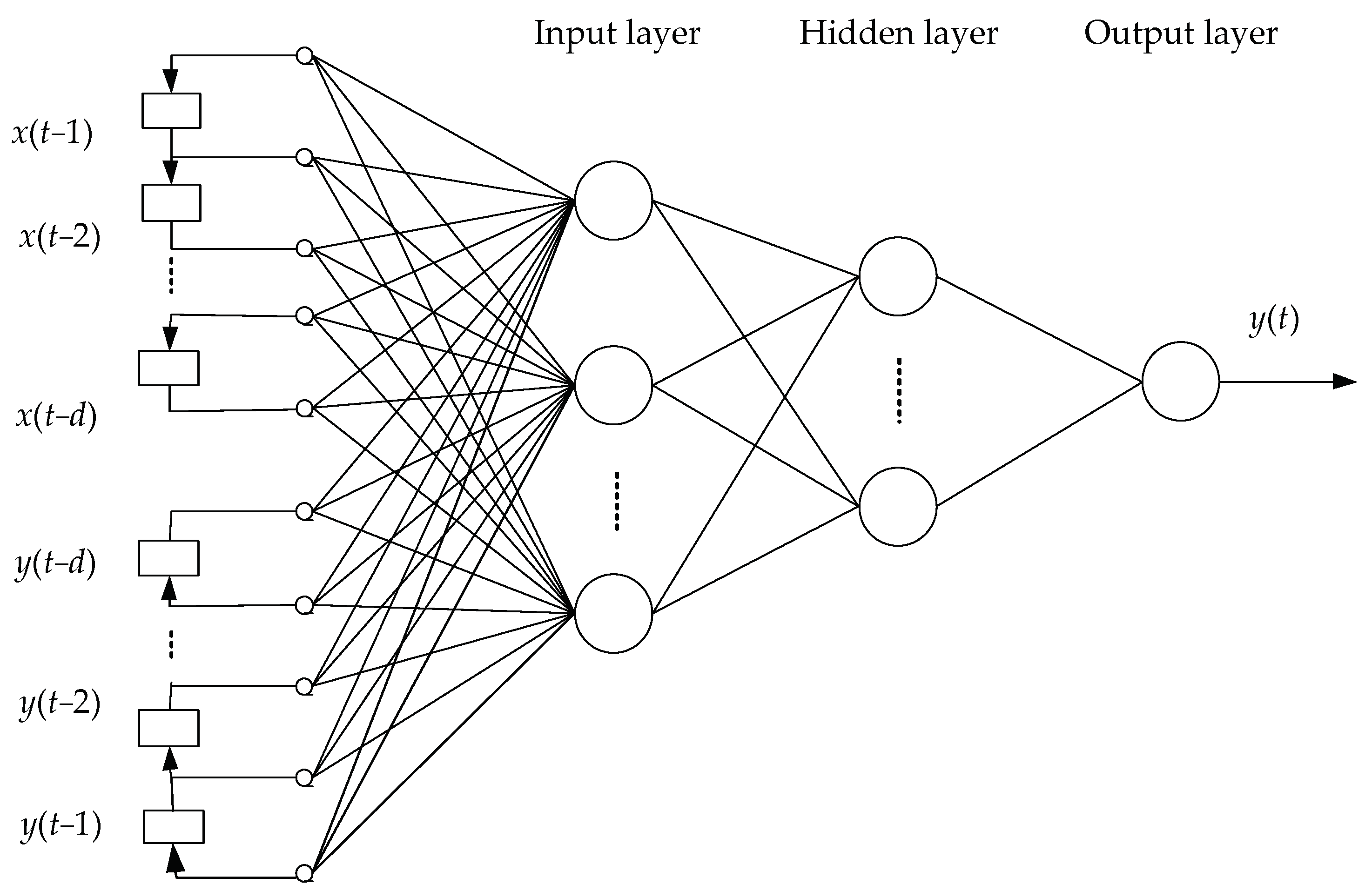
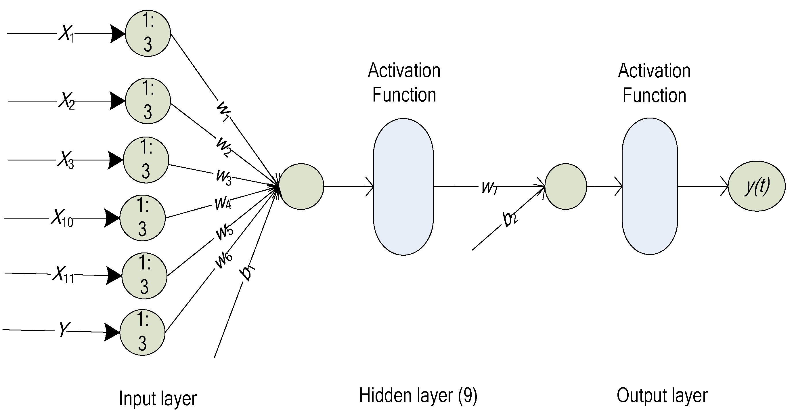
2.2. NARX Neural Network

The water consumption sequence is a dynamic nonlinear sequence. The NARX neural network is a kind of dynamic RNN. It introduces the concept of time series, which makes the NARX model have good dynamic characteristics and high anti-interference ability. The basic network structure of the NARX neural network is the same as that of the ANN. The ANN is a mathematical model that imitates the structure and function of biological neural networks [27]. In general, an ANN consists of an input layer, one or more hidden layers, and an output layer, through which the results are provided [28]. It is noted that each layer has several neurons.
Neural networks that use feedback connections, enabling lateral or backward information flow within the network, are called RNNs. The NARX neural network model is a special type of RNN that uses global feedback connection between the output layer and the input layer. This makes the NARX neural network have good dynamic characteristics and strong anti-interference ability [29]. The NARX neural network is a neural network with the memory function. The output of this network depends on the current input and past output, which greatly improves the generalization ability of the network.
The NARX model not only has the advantages of the traditional time-series model but also can improve adaptability of the model’s nonlinear data through training. It introduces the output vector’s delay feedback into the network training to form a new input vector [30]. The NARX model (open loop) is defined as follows:
y ( t ) = f [ y ( t 1 ) , y ( t 2 ) , ... , y ( t d ) , x ( t 1 ) , x ( t 2 ) , ... , x ( t d ) ]
where y(.) refers to water consumption and x(.) refers to an external factor in this paper. The x(t) indicates the value of x at time t, and d is the number of delays.
The model structure of NARX neural network is shown in Figure 1.
The activation function g(.) (sigmoid function [31] selected in this paper) can amplify the output of the neuron or limit it to a suitable range. Hence Equation (7) can be re-written as:
y ( t ) = g ( i = t d t 1 w i x ( i ) + i = t d t 1 w ¯ i y ( i ) + b )
where wi and w ¯ i are weights, and b represents the bias.
The sigmoid function is:
g ( u ) = 1 1 + e u
where u is the neuron input.

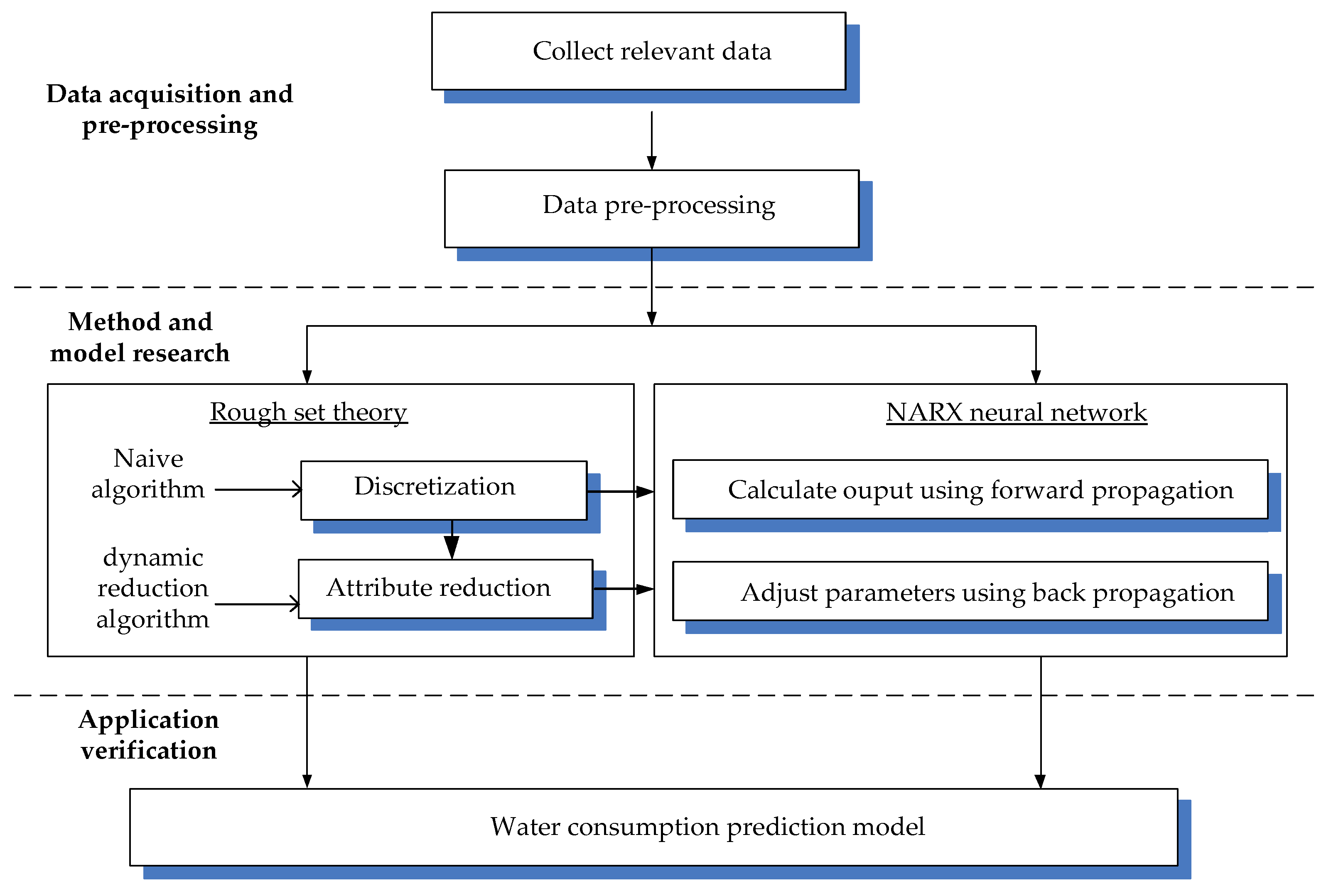
2.3. A Water Consumption Prediction Model Based on the RS–NARX Neural Network

In this section, the prediction model incorporating RS and NARX neural networks is constructed. The main process of the proposed model is illustrated in Figure 2.
The main steps of the process of the RS–NARX neural network are described as follows:
Step 1:
Data preparation. Collect relevant data.
Step 2:
Data discretization. The continuous data is discretized using the Naive algorithm [32].
Step 3:
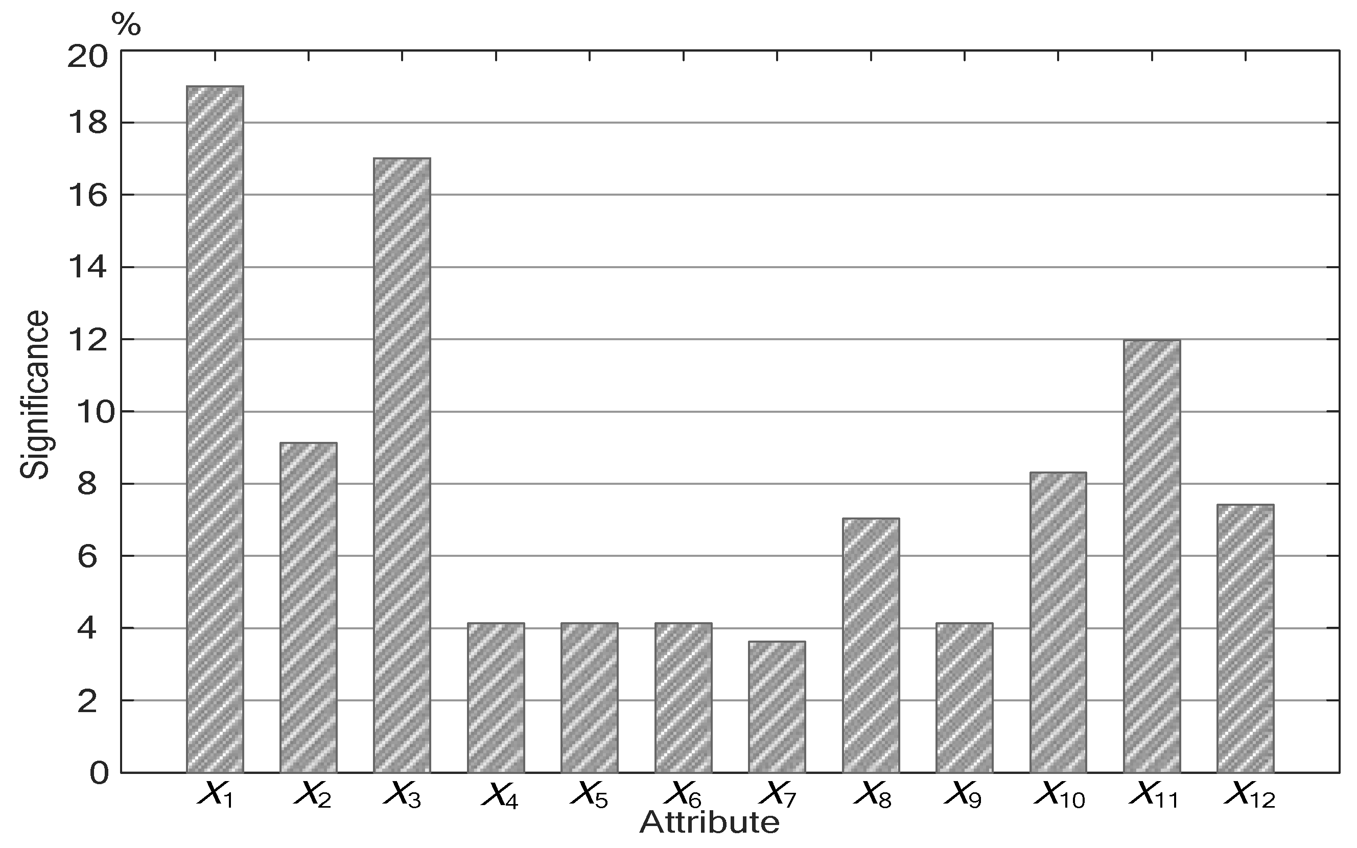
Attribute reduction. The dynamic reduction algorithm [33] is used to perform attribute reduction, and the importance of each attribute is obtained.
Step 4:
Train the NARX neural network.
(1)
Establish a NARX network structure.
(2)
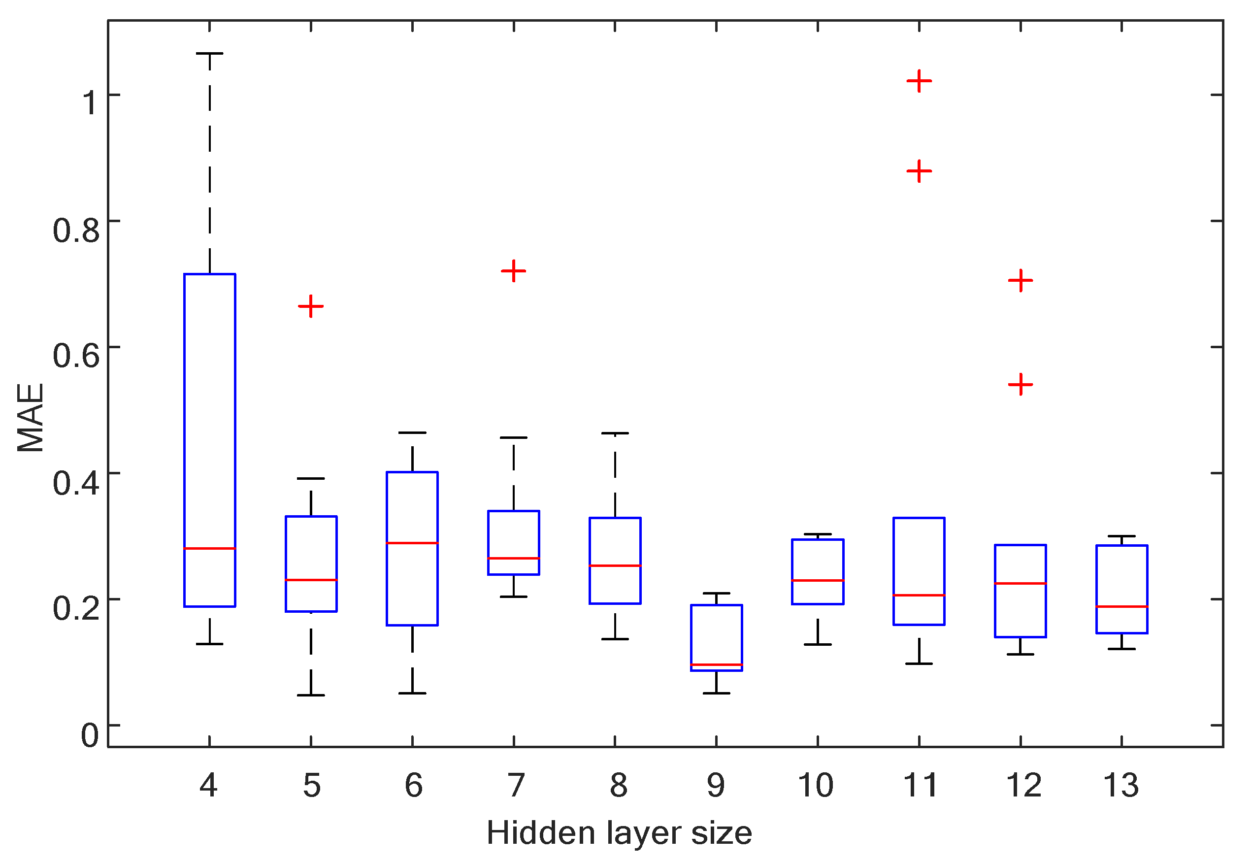
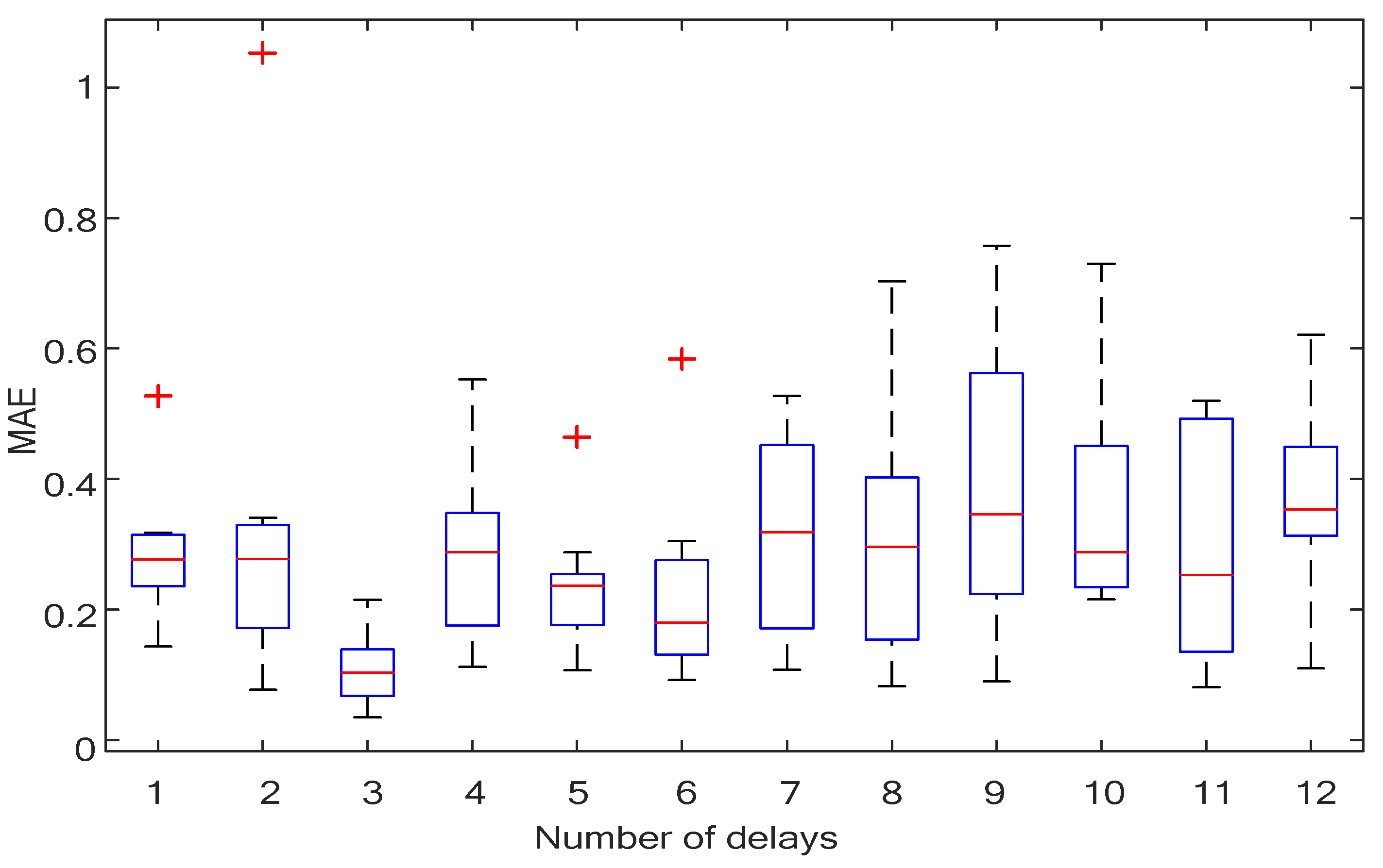
Determine the parameters (the number of hidden layers and the number of delays) in the NARX neural network.
(3)
Train the NARX neural network.
Step 5:
Obtain the predicted value.

3. Data Description and Evaluation Indexes

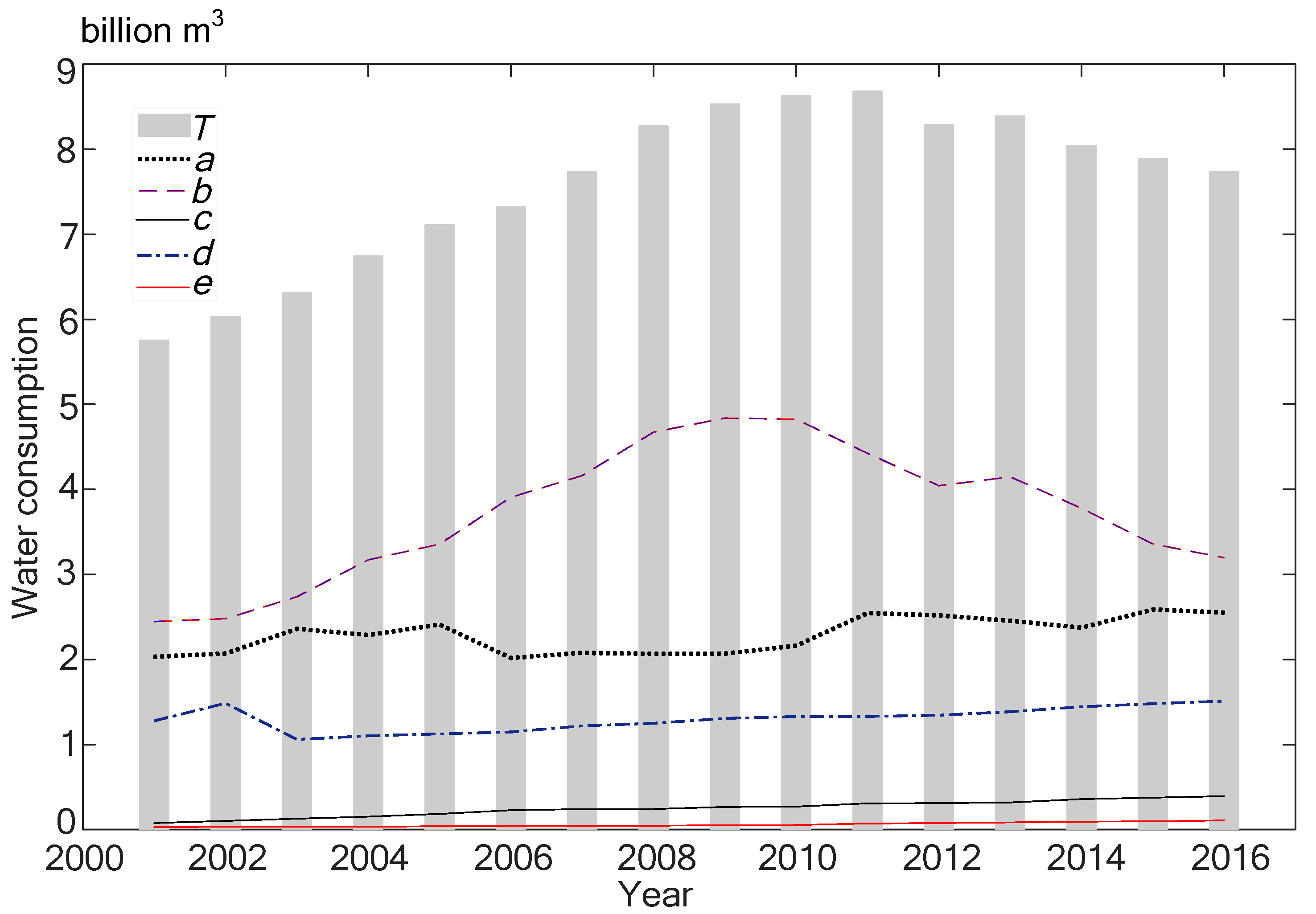
3.1. Data Description

Chongqing is one of the four municipalities under direct control of the central government of China. As the largest heavy industrial and commercial city in the southwest of China, Chongqing is an important link between “the Belt and Road” and the Yangtze River economic belt. Chongqing is a serious water shortage area. In recent years, water waste, water pollution and other problems are widespread in Chongqing, which has become the main bottleneck restricting the sustainable development of the economy and society. Therefore, Chongqing is used as a case study to provide advice on water resources management in the country. The study collected annual data including total water consumption and condition attributes (social and economic factors) including the effective irrigation area (103 hectares), agricultural GDP (108 RMB), precipitation (billion m3), industrial GDP (108 RMB), urbanization rate (%), service industry GDP (108 RMB), residential water price (ton/RMB), population (104 persons), residential consumption level (RMB), agricultural output ratio (%),industrial output ratio (%) and service industrial output ratio (%). The water consumption and socio-economic data of Chongqing from 2001 to 2016 were collected from Chongqing Water Resources Bulletin [34] and the Statistical Yearbook of Chongqing [35], respectively. Table 1 presents the values of socio-economic indicators of Chongqing in 2001–2016.
The total water consumption (billion m3) is divided into agricultural water consumption (billion m3), industrial water consumption (billion m3), service industry water consumption (billion m3), domestic water consumption (billion m3) and eco-environmental water consumption (billion m3). The water consumption in each sector in Chongqing from 2001 to 2016 is illustrated in Figure 3. The total water consumption has gradually increased from 2001 to 2011 and has had a gradual downward trend since 2012. In May 2012, the Ministry of Water Resources convened the national work conference on water resources, assigning the tasks for implementing the strictest water resources management system. According to the instructions of the State Council, Chongqing Municipality has also begun to implement the strictest water resources management system in Chongqing. As shown in Figure 4, industrial water consumption began to decrease in 2010. During the “Twelfth Five-Year Plan” period, the Chongqing Municipal Government completed the task of industrial restructuring and eliminating the outdated production capacity. This is the main reason for the decline of water use in the secondary industry during the period 2010–2015 (the “12th Five-Year Plan” period). The water consumption has decreased, however GDP has been increasing year by year. This indicates that various industries have increased the utilization of water resources and reduced unnecessary water use. Of course, the most stringent water resources management system is indispensable. The strictest water resources management system emphasizes strict control of water consumption, optimization of water resources allocation, and overall improvement of water use efficiency. Therefore, under the premise of controlling the total water consumption, it is necessary to coordinate the water resources allocation of each sector. Agriculture and industry are the main sectors in terms of water consumption. Agricultural and industrial water consumption accounts for 79% of total water consumption. Third is residential water consumption, which accounts for 17% of total water consumption.

3.2. Evaluation Indexes

In this paper, the following evaluation indicators are selected: mean absolute error (MAE), mean absolute percent error (MAPE) and root mean square error (RMSE). The MAE, MAPE and RMSE are all common measures of forecasting error in time-series analysis. The formulas are as follows:
E MAE = 1 n t = 1 n | y o , ( t ) y m , ( t ) | ,
E MAPE = 100 n t = 1 n | ( y o , ( t ) y m , ( t ) ) y o , ( t ) | ,
E RMSE = 1 n t = 1 n ( y o , ( t ) y m , ( t ) ) 2 ,
where yo,(t) represents the observed value of y at time t and ym,(t) represents the predicted value of y at time t.

4. Experimental Results and Analysis

4.1. The Attribute Reduction in Water Consumption Based on the Rough Set

Since the RS lacks direct and efficient processing for continuous data, the continuity data need to be discretized before the attribute reduction (discrete data do not need to be discretized). First, the width discretization method [36] was used to discretize the decision attributes. The formula for the breaking point interval I is provided below:
I = ( x max x min ) / k ,
where xmax is the maximum value in the series, xmin is the minimum value in the series, and k is the given parameter, which is the number of intervals.
The total water consumption fluctuates from approximately 5.5 billion m3 to 9 billion m3 with the interval length 3.5 billion m3. Hence it is divided into seven equidistant intervals. The discretization method is presented in Table 2.
According to the interval and assignment given in Table 2, the discretization results of decision attributes (water consumption) were obtained. The results are provided in Table 3.
The equal width discretization method is a division of the continuous variable value and does not need to consider the variable value of the decision table. Naive Bayes has a solid mathematical foundation and it is a heuristic algorithm that discretizes the continuous condition attributes based on decision attributes. Due to the indistinguishable relationship between condition attributes and decision attributes, the Naive algorithm is used to discretize the continuous condition attributes to obtain a better discretization effect. The results of the discretization are presented in Table 4.
After the data were discretized, the rough set theory was used for attribute reduction. X1 to X12 are condition attributes, and total water consumption is a decision attribute. There are many algorithms for condition attribute reduction, and the dynamic reduction algorithm can be said to be a very stable reduction algorithm. The principle of dynamic reduction is to randomly sample a sub-table from a given decision table and then determine the reduction. It adds or removes the condition attribute to the sampled sub-table to correct the reduction result, which effectively enhance the anti-noise ability of the reduction. This article uses dynamic reduction algorithms for attribute reduction. The number of the sampling level is five. The weighted average is based on the frequency of occurrence of the attribute, and the importance of the influencing factors on the water consumption is obtained. The result is illustrated in Figure 4.
As shown in Figure 4, X1 is the most important influencing factor on the decision attribute. X1 reflected drought resistance of cultivated land indirectly, that is, when X1 expands, the water use efficiency increases and the water consumption decreases. In addition, X1 directly affects the water consumption of the primary industry. As shown in Figure 3, the primary industry and the secondary industry are the main water sectors. Furthermore, X2, X10 and X11 are the key factors that cannot be omitted. The X3 in the condition attributes is also highly important. Rainwater can replenish cultivated land and forest land. People can also recycle water resources through rainwater harvesting systems. In summary, based on the combination of qualitative and quantitative analyses, condition attributes with an importance greater than 8% should be selected, that is, X1 (effective irrigation area), X2 (agricultural GDP), X3 (precipitation), X10 (agricultural output ratio) and X11 (industrial output ratio). The selected condition attribute is used as a factor for predicting water consumption and input into the prediction model.

4.2. The RS-NARX Neural Network
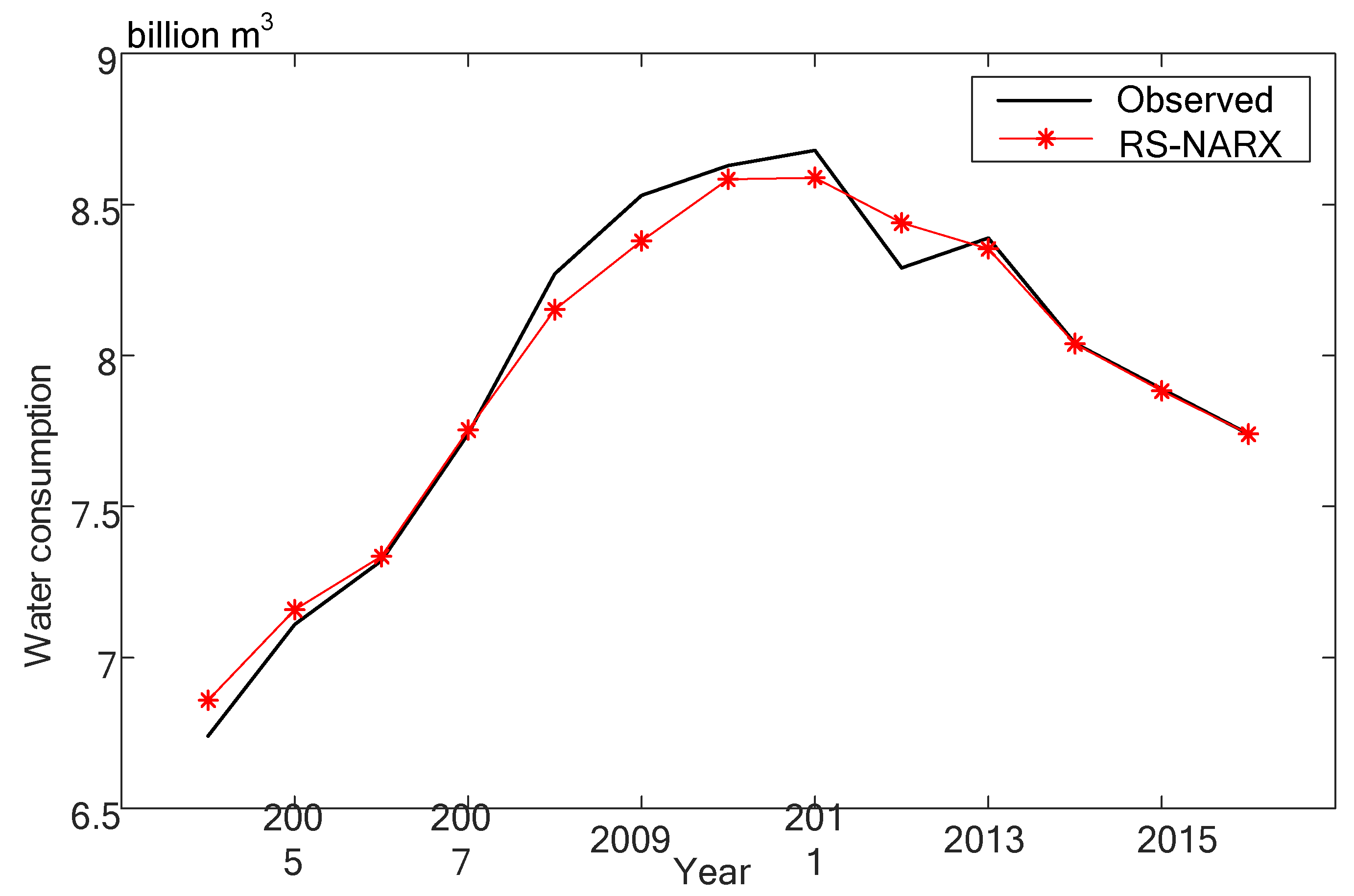
For the NARX modeling, the data from 2001 to 2013 were used to train the model, and the data from 2014 to 2016 were used to test the model. The commonly used empirical formula was used to determine the range of hidden layer neurons [37]. The formula is as follows:
H = m + n + a
where H represents the number of hidden neurons, m represents the number of input neurons, n represents the number of output neurons, and a is a constant between 1 and 10.
As such, the range of hidden neurons is 4–13. To get the optimal parameters, each value was tested 10 times. Thus, the prediction error range corresponding to each parameter value was obtained. The MAE was used to measure the error. The smaller the MAE value was, the smaller the prediction error was. The more dispersed the distribution of MAE was, the more unstable the prediction results were, and vice versa. Here, a box plot is used to show the results of the experiment, which is shown in Figure 5. The choice of the number of neurons in the hidden layer directly affects the prediction result of water consumption. When the number of neurons in the hidden layer is 4, the experimental error is large, and the result is unstable. As the number of neurons in the shadow layer increases, the prediction results become better. When the number of hidden layer neurons is 9, the prediction result is the best. Therefore, the number of hidden neurons in the NARX neural network is set to nine.
The number of delays d is a parameter that determines the input delay and the output feedback delay. A reasonable use of delay parameters can make full use of the inherent law of time series and thus better predict water consumption. The range of d is determined by the length of the training set (length = 13, i.e., values in 2001–2013), so d is set as 1–12 for modeling investigation. Similarly, to select the best number of delays, the d was found through experiments. Each value was repeated 10 times, and all the results are illustrated in Figure 6. It can be seen from the box plot that when the delay order is three, the prediction performance is the best and is more stable.
Based on the above tests, it is found that when the number of delays is three (that is, using the data for the first three years to predict the water consumption in the following year as a cycle), the prediction result is good. Therefore, y(t) is determined by the following variables:
y ( t ) = f [ y ( t 1 ) , y ( t 2 ) , y ( t 3 ) , x ( t 1 ) , x ( t 2 ) , x ( t 3 ) ] .
After all of the parameters determined, the trained NARX neural network framework is illustrated in Figure 7. In Figure 7, Y = [y(t − 1), y(t − 2), y(t − 3)] refers to the delayed feedback vector.
After setting up the neural network structure, the RS–NARX neural network model is trained. The Nested Cross-Validation (NCV) method is used to test the model [38]. A method based on Forward-Chaining is used to cross-validate time series data to avoid data leakage. The triennial data is taken as the test set, and all the previous data is assigned to the training set. In this experiment, the delay number d is three. The average results are illustrated in Figure 8. The proposed RS–NARX neural network model predicts the trend of water consumption accurately. However, the prediction of the abrupt nodes in water consumption needs to be improved. At the beginning, the total water consumption used has been increasing year by year. With the development of the population and the economy, the demand for water has also increased. Since 2010, water consumption has started to decrease, which contradicts the growth in the population and the economy. This is mainly a result of the guiding policies of the government during the Twelfth Five-Year Plan period, during which the government vigorously promoted the water conservation policy. The most stringent water management system was introduced in 2012, which led to a sharp drop in water consumption in 2012. Overall, the prediction of the RS–NARX neural network model is very good. The following is a detailed analysis of the prediction results from the error of each year.
The error of the prediction results are illustrated in Figure 9. There are large errors in several nodes of the training set (i.e., values in year 2009 and 2012). Unpredictable policy impacts occurred in 2012, which led to a major bias in water consumption forecasting. Additionally, the forecasting error of 2013–2016 decreased year by year. Driven by strong policies, the gradual reduction in water consumption has stabilized. This is the main reason for the high prediction accuracy. Overall, the error of all predicted nodes is controlled within 0.2. The predicted results are acceptable.

4.3. Comparison

To prove the superiority of the RS–NARX neural network model, a single NARX neural network model (without RS) and the BPNN model were chosen as references. Similarly, the parameters of the comparison model were obtained experimentally (repeat the experiment 10 times for each value to obtain the best parameters). Table 5 shows the parameter settings of the comparison models. Among them, “Hidden layer size” represents the number of neurons in hidden layer.
Similarly, the comparison model is tested using the NCV method. The results of the compared models are illustrated in Figure 10. The prediction results of the comparison model are not as accurate as those of the RS–NARX model. The prediction results of the NARX model are more accurate than those of the BPNN. The single NARX neural network model performed poorly on the prediction of the mutated node. Therefore, the use of rough set theory makes the input data set more streamlined, which removes redundant information, and successfully improves the prediction accuracy of the NARX neural network model. This is the reason why NARX neural network model is better adapted to the mutation nodes of nonlinear dynamic data. As can be seen from the prediction results of the BPNN model, a certain node change from the original data causes a change in the overall prediction trend. This is disadvantageous for the prediction of nonlinear dynamic data.
To analyze the error distribution of the comparison models more easily, the error of each node of the two comparison models is provided. The prediction errors of the comparison models are illustrated in Figure 11. The error of the comparison model is large. At some nodes, the BPNN model has greater error results than a single NARX neural model. The prediction errors of the single NARX neural network model in 2011 and 2015 exceed 0.2. In the prediction results of the BPNN model, the prediction errors of six nodes are all above 0.2. The prediction errors in 2006 even exceed 0.4.
Table 6 lists the errors of the different models. As shown in Table 6, the RS–NARX neural network model has higher accuracy. The RS theory is used to pre-process the data set, thus reducing the interference of unnecessary data to the model. In addition, the NARX neural network has the memory function of the dynamic neural network, so nonlinear dynamic data can be better fitted. Hence the proposed framework improves the prediction accuracy of the model. In short, the rank of these models is RS–NARX (best), NARX, and BPNN (worst). Therefore, the proposed RS–NARX neural network model is effective in forecasting water consumption.

5. Conclusions

In this paper, the proposed RS–NARX neural network model is reported to predict the water consumption of Chongqing. First, the RS theory is used to reduce the attribute, and the key influence factors of water consumption are obtained. The reduction results are used as the inputs of the predictive model, and the NARX neural network model is used to predict water consumption. The results indicate that the proposed model is more accurate than a single NARX model and a BPNN model.
The proposed RS–NARX neural network model combines the advantages of the RS theory with those of NARX neural networks. The RS theory removes information redundancy and improves the prediction efficiency and accuracy of NARX neural networks, so that the NARX neural network model can better fit the nonlinear dynamic sequence. The results of predicting water consumption using the RS–NARX model are satisfactory. The results can provide recommendations for the allocation of water resources.

Author Contributions

Writing—original draft preparation, Y.Z.; conceptualization, J.X.; data curation, W.Z.; funding acquisition, Q.L. and J.X.; writing—review and editing, W.Z. All authors have read and agreed to the published version of the manuscript.

Funding

This work is supported by the Open Fund of Chongqing Technology and Business University with No. KFJJ2018106.

Institutional Review Board Statement

Not applicable.

Informed Consent Statement

Not applicable.

Data Availability Statement

Chongqing Water Resources Bulletin. Available online: http://slj.cq.gov.cn (accessed on 30 September 2020); Statistical Yearbook of Chongqing. Available online: http://tjj.cq.gov.cn (accessed on 3 April 2020).

Acknowledgments

The authors would like to thank precious suggestions by all anonymous reviewers and LetPub editing (https://www.letpub.com.cn/), which have greatly helped with the improvement of the paper.

Conflicts of Interest

The authors declare no conflict of interest.

References

  1. Brentan, B.M.; Luvizotto, E., Jr.; Herrera, M.; Izquierdo, J.; Rafael, P.G. Hybrid regression model for near real-time urban water demand forecasting. J. Comput. Appl. Math. 2017, 309, 532–541. [Google Scholar] [CrossRef]
  2. Bai, Y.; Wang, P.; Li, C.; Xie, J.; Wang, Y. A multi-scale relevance vector regression approach for daily urban water demand forecasting. J. Hydrol. 2014, 517, 236–245. [Google Scholar] [CrossRef]
  3. Kang, H.S.; Kim, H.; Lee, J.; Lee, L.; Kwak, B.Y.; Lm, H. Optimization of pumping schedule based on water demand forecasting using combined model of autoregressive integrated moving average and exponential smoothing. Water Sci. Technol. Water Supply 2015, 15, 188–195. [Google Scholar] [CrossRef]
  4. Cheng, Z.W.; Li, X.; Bai, Y.; Li, C. Multi-scale fuzzy inference system for influent characteristics prediction of wastewater treatment. CLEAN-Soil Air Water 2018, 46, 1700343. [Google Scholar] [CrossRef]
  5. Al-Zahrani, M.A.; Abo-Monasar, A. Urban residential water demand prediction based on artificial neural networks and time series models. Water Resour. Manag. 2015, 29, 3651–3662. [Google Scholar] [CrossRef]
  6. Chen, G.; Long, T.; Bai, Y.; Zhang, J. A forecasting framework based on Kalman filter integrated multivariate local polynomial regression and relevance vector regression method: Application to urban water demand. Neural Process. Lett. 2019, 50, 497–513. [Google Scholar] [CrossRef]
  7. Suh, D.; Ham, S. A water demand forecasting model using BPNN for residential building. Contemp. Eng. Sci. 2016, 9, 1–10. [Google Scholar] [CrossRef]
  8. Zubaidi, S.L.; Dooley, J.; Alkhaddar, R.M.; Abdellatif, M.; AL-Bugharbee, H.; Martorell-Ortega, S. A novel approach for predicting monthly water demand by combining singular spectrum analysis with neural networks. J. Hydrol. 2018, 561, 136–145. [Google Scholar] [CrossRef]
  9. Rezaali, M.; Quilty, J.; Karimi, A. Probabilistic urban water demand forecasting using wavelet-based machine learning models. J. Hydrol. 2021, 600, 126358. [Google Scholar] [CrossRef]
  10. Altunkaynak, A.; Nigussie, T.A. Monthly water demand prediction using wavelet transform, first-order differencing and linear detrending techniques based on multilayer perceptron models. Urban Water J. 2018, 15, 177–181. [Google Scholar] [CrossRef]
  11. Chen, P.A.; Chang, L.C.; Chang, F.J. Reinforced recurrent neural networks for multi-step-ahead flood forecasts. J. Hydrol. 2013, 497, 71–79. [Google Scholar] [CrossRef]
  12. Bai, Y.; Bezak, N.; Zeng, B.; Li, C. Sapač, K.; Zhang, J. Daily runoff forecasting using a cascade long short-term memory model that considers different variables. Water Resour. Manag. 2021, 35, 1167–1181. [Google Scholar] [CrossRef]
  13. Salloom, T.; Kaynak, O.; He, W. A novel deep neural network architecture for real-time water demand forecasting. J. Hydrol. 2021, 599, 126353. [Google Scholar] [CrossRef]
  14. Peronaci, S.; Taravat, A.; Frate, F.D.; Oppelt, N. Use of NARX neural networks for Meteosat Second Generation SEVIRI very short-term cloud mask forecasting. Int. J. Remote Sens. 2016, 37, 6205–6215. [Google Scholar] [CrossRef]
  15. Wunsch, A.; Liesch, T.; Broda, S. Forecasting groundwater levels using nonlinear autoregressive networks with exogenous input (NARX). J. Hydrol. 2017, 1–16. [Google Scholar] [CrossRef]
  16. Mousavi-Mirkalaei, P.; Banihabib, M. An ARIMA-NARX hybrid model for forecasting urban water consumption (case study: Tehran metropolis). Urban Water J. 2019, 16, 1–12. [Google Scholar] [CrossRef]
  17. Xu, Y.B.; Zhang, J.; Long, Z.; Lv, M. Daily urban water demand forecasting based on chaotic theory and continuous deep belief neural network. Neural Process. Lett. 2019, 50, 1173–1189. [Google Scholar] [CrossRef]
  18. Howe, C.W. Getting western municipal water prices right: Reflecting the scarcity value of water. J. Am. Water Work. Assoc. 2017, 109, 47–49. [Google Scholar] [CrossRef]
  19. Slavíková, L.; Malý, V.; Rost, M.; Petružela, L.; Vojáček, O. Impacts of climate variables on residential water consumption in the Czech Republic. Water Resour. Manag. 2013, 27, 365–379. [Google Scholar] [CrossRef]
  20. Angulo, A.; Atwi, M.; Barberán, R.; Mur, J. Economic analysis of the water demand in the hotels and restaurants sector: Shadow prices and elasticities. Water Resour. Res. 2015, 50, 6577–6591. [Google Scholar] [CrossRef]
  21. Zhang, W.J.; Yu, Y.; Zhou, X.Y.; Yang, S.; Li, C. Evaluating water consumption based on water hierarchy structure for sustainable development using grey relational analysis: Case study in Chongqing, China. Sustainability 2018, 10, 1538. [Google Scholar] [CrossRef] [Green Version]
  22. Yu, T.T.; Yang, S.; Bai, Y.; Gao, X.; Li, C. Inlet water quality forecasting of wastewater treatment based on kernel principal component analysis and an extreme learning machine. Water 2018, 10, 873. [Google Scholar] [CrossRef] [Green Version]
  23. Li, C.; Cerrada, M.; Cabrera, D.; Sanchez, R.V.; Pacheco, F.; Ulutagay, G.; Oliveira, J.V. A comparison of fuzzy clustering algorithms for bearing fault diagnosis. J. Intell. Fuzzy Syst. 2018, 34, 3565–3580. [Google Scholar] [CrossRef]
  24. Liu, J.Q.; Cheng, W.P.; Zhang, T.Q. Principal factor analysis for forecasting diurnal water-demand pattern using combined rough-set and fuzzy-clustering technique. J. Water Resour. Plan. Manag. 2013, 139, 23–33. [Google Scholar] [CrossRef]
  25. Hu, J.; Li, T.; Luo, C.; Fujita, H.; Yang, Y. Incremental fuzzy cluster ensemble learning based on rough set theory. Knowl.-Based Syst. 2017, 132, 144–155. [Google Scholar] [CrossRef]
  26. Vidhya, K.A.; Geetha, T.V. Rough set theory for document clustering: A review. J. Intell. Fuzzy Syst. 2017, 32, 2165–2185. [Google Scholar] [CrossRef]
  27. Gebler, D.; Wiegleb, G.; Szoszkiewicz, K. Integrating river hydromorphology and water quality into ecological status modelling by artificial neural networks. Water Res. 2018, 139, 395. [Google Scholar] [CrossRef]
  28. Cutore, P.; Campisano, A.; Kapelan, Z.; Modica, C.; Savic, D. Probabilistic prediction of urban water consumption using the SCEM-UA algorithm. Urban Water J. 2008, 5, 125–132. [Google Scholar] [CrossRef]
  29. Matkovskyy, R.; Bouraoui, T. Application of neural networks to short time series composite indexes: Evidence from the nonlinear autoregressive with exogenous inputs (NARX) model. J. Quant. Econ. 2018, 1, 1–14. [Google Scholar] [CrossRef]
  30. Chatterjee, S.; Nigam, S.; Singh, J.B.; Upadhyaya, L.N. Software fault prediction using Nonlinear Autoregressive with eXogenous Inputs (NARX) network. Appl. Intell. 2012, 37, 121–129. [Google Scholar] [CrossRef]
  31. Yoshifusa, I. Approximation of functions on a compact set by finite sums of a sigmoid function without scaling. Neural Netw. 1991, 4, 817–826. [Google Scholar] [CrossRef]
  32. Li, J.F.; Xu, E. Improvement of Naive Scaler. Comput. Eng. Des. 2009, 30. Available online: https://en.cnki.com.cn/Article_en/CJFDTotal-SJSJ200913035.htm (accessed on 30 September 2020).
  33. Moudani, W.; Chahine, A.; Chakik, F.; Mora-Camino, F. Dynamic rough sets features reduction. Int. J. Comput. Sci. Inf. Secur. 2014, 9, 355–358. [Google Scholar] [CrossRef]
  34. Chongqing Water Resources Bulletin. Available online: http://slj.cq.gov.cn (accessed on 30 September 2020).
  35. Statistical Yearbook of Chongqing. Available online: http://tjj.cq.gov.cn (accessed on 3 April 2020).
  36. Orhan, U.; Hekim, M.; Özer, M. Epileptic seizure detection using artificial neural network and a new feature extraction approach based on equal width discretization. J. Fac. Eng. Archit. Gazi Univ. 2011, 26, 575–580. [Google Scholar]
  37. Li, X.L.; Yuan, J.M. Research classification of Jujube based on BP artificial neural network. J. Chem. Pharm. Res. 2015, 7, 486–489. [Google Scholar]
  38. Varma, S.; Simon, R. Bias in error estimation when using cross-validation for model selection. BMC Bioinform. 2006, 7, 91. [Google Scholar] [CrossRef] [Green Version]
Figure 1. Architecture of the NARX neural network.
Water 14 00329 g001
Figure 2. Process of NARX neural network with RS.
Water 14 00329 g002
Figure 3. Water consumption of each water sectors in Chongqing from 2001 to 2016, where T is total water consumption (billion m3), a is agricultural water consumption (billion m3), b is industrial water consumption (billion m3), c is service industry water consumption (billion m3), d is domestic water consumption (billion m3) and e is eco-environmental water consumption (billion m3).
Water 14 00329 g003
Figure 4. Importance of condition attributes.
Water 14 00329 g004
Figure 5. Calculate the dependence of the MAE on the size of the hidden layer.
Water 14 00329 g005
Figure 6. Calculate the dependence of the MAE on the number of delays.
Water 14 00329 g006
Figure 7. Structure of NARX neural network.
Water 14 00329 g007
Figure 8. Result of RS-NARX neural network.
Water 14 00329 g008
Figure 9. Error analysis using RS-NARX neural network.
Water 14 00329 g009
Figure 10. Results of the comparison models.
Water 14 00329 g010
Figure 11. Error analysis using comparison models.
Water 14 00329 g011
Table 1. Statistics on water consumption and socio-economic indicators for Chongqing in 2001–2016.
YearX1X2X3X4X5X6X7X8X9X10X11X12
2001631.93294.9057.40841.9537.40840.011.672829.212937154342
2002641.16317.8797.49958.8739.90956.122.422814.833204144343
2003649.69339.06101.331135.3141.901081.352.462803.193591134442
2004616.79428.0598.591376.9143.501229.622.482793.324155144541
2005618.09463.4093.201564.0045.201440.322.662798.004702134542
2006621.32386.3876.581871.6546.701649.202.662808.005323104842
2007633.67482.39104.562368.5348.301825.212.802816.006453105139
2008658.86575.4097.873057.7850.002160.482.802839.007637105337
2009672.02606.8084.833448.7751.602474.442.802859.00849495338
2010685.25685.3887.204359.1253.002881.082.902884.62972395536
2011692.88844.5289.965543.0455.003623.813.102919.0011,83285536
2012702.97940.0189.045975.1856.984494.413.502945.0013,65585239
2013675.181002.6887.645812.2958.345968.293.502970.0015,42384547
2014677.261061.03104.656529.0659.606672.513.502991.4017,26274647
2015687.191150.1586.387069.3760.947497.753.503016.5518,86074548
2016690.601303.24101.917898.9262.598538.433.503048.0021,03274548
Note: X1 represents effective irrigation area (103 hectares), X2 represents agricultural GDP (108 Yuan), X3 represents precipitation (billion m3), X4 represents industrial GDP (108 RMB), X5 represents urbanization rate (%), X6 represents service industry GDP (108 RMB), X7 represents residential water price (ton/RMB), X8 represents population (104 persons), X9 represents residential consumption level (RMB), X10 represents agricultural output ratio (%), X11 represents industrial output ratio (%), and X12 represents service industrial output ratio (%).
Table 2. Discretization interval assignment of total water consumption.
IntervalValueIntervalValue
[5.5, 6)1[6, 6.5)2
[6.5, 7)3[7, 7.5)4
[7.5, 8)5[8, 8.5)6
[8.5, 9)7
Table 3. Results of decision attribute discretization.
Year20012002200320042005200620072008
Value12234456
Year20092010201120122013201420152016
Value77766655
Table 4. Result of condition attribute discretization.
UX1X2X3X4X5X6X7X8X9X10X11X12
2001111111121112
2002212111111113
2003213111111112
2004113111111122
2005122111111122
2006111222112222
2007123222222231
2008222222222231
2009221222222231
2010321222222231
2011322222222331
2012332333333331
2013232333333323
2014233333333323
2015331333333323
2016333333333323
Table 5. Parameter setting of the comparison models.
ParameterNARXBPNN
Hidden layer size1010
Number of delays3None
Table 6. Comparison of the training and testing errors of the three models.
ModelMAE (Billion m3)MAPE (%)RMSE (Billion m3)
BPNN0.1856 ± 0.16652.3855 ± 0.02210.2451 ± 0.0980
NARX0.1135 ± 0.14711.4253 ± 0.01840.1813 ± 0.0798
RS-NARX0.0611 ± 0.05470.7636 ± 0.20220.0821 ± 0.0218
Publisher’s Note: MDPI stays neutral with regard to jurisdictional claims in published maps and institutional affiliations.

