Analytical Solution for Fractional Well Flow in a Double-Porosity Aquifer with Fractional Transient Exchange between Matrix and Fractures

Abstract

An analytical solution is presented for groundwater flow to a well in an aquifer with double-porosity behavior and transient transfer between fractures and matrix. The solution is valid for fractional flow dimensions including linear, cylindrical or spherical flow to the well and for fractional inter-porosity diffusive transfer including release from storage in infinite slabs, infinite cylinders or spherical matrix blocks. Approximations are also presented for small and large times that are easy to evaluate in practice. The solution can be used to analyze pumping tests via coupling with a parameter estimation code. The utility of the method is demonstrated by a practical example using data from a pumping test performed in a fractured chalk aquifer. The analytical solution allows the accurate modeling of pumping tests and the estimation of aquifer parameters that are statistically significant and physically relevant.

1. Introduction

The concept of double (or dual) porosity explains groundwater flow in fractured aquifers, by considering the matrix as a primary porous system with low hydraulic conductivity and high storage capacity and the fractures as a secondary porous system with high hydraulic conductivity and low storage capacity [1]. Groundwater thus mainly flows through the fractures while the rock matrix releases fluid to the fractures at a limited rate due to its low permeability. In a pumping test, the drawdown in the fractures shows typical characteristics inherent in double-porosity behavior. Initially, the flow to the well consists of fluid released from storage in the fractures as if the rock matrix were non-existing, but gradually water is also released from storage in the matrix and eventually the aquifer acts as a homogeneous system with the storage capacity of the fractures and matrix combined.

Two approaches have been proposed to quantify the exchange of water between the fractures and the matrix: (1) pseudo-steady-state flow assuming an exchange rate proportional to the difference in hydraulic head between the fractures and the matrix [1,2,3], and (2) transient flow where the exchange rate is determined by diffusive flow in the matrix blocks to the fractures [4,5,6]. Applications show that both approaches have their merits [6,7,8], as the pseudo-steady-state approach has the advantage of mathematical simplicity, while the transient approach is superior from a theoretical and physical point of view.

In the transient flow approach, the geometry of the matrix blocks is schematized in regular basic shapes such as slabs, cylinders, cubes or spheres. Kazemi [4] considered infinite parallel slabs and presented a numerical solution using a finite difference technique. This problem was later solved analytically by Boulton and Streltsova [5]. An approximate solution for cubic matrix blocks was presented by de Swaan [9]. Bourdet and Gringarten [6] derived approximate solutions for matrix slabs and for spherical matrix blocks, which also include wellbore storage and skin effects. Moench [8] developed semi-analytical solutions for slabs and for spherical matrix blocks with skin resistance that impedes the exchange between fractures and matrix. Barker and Black [10] presented a semi-analytical solution for flow to a large diameter well in a fractured aquifer with slab matrix blocks; this solution was extended by Barker [11] to matrix blocks in the form of cylinders or spheres. Barker [12] presented matrix block geometry functions for several shapes and mixtures and concluded that the long-time asymptotic behaviour is independent of the block geometry and accords with the pseudo-steady-state approach.

Barker [13] presented an analytical solution for well flow in single-porosity systems characterized by fractional flow dimensions. Hamm and Bidaux [14] extended this approach and presented a semi-analytical solution for fractional flow to wells in double-porosity systems with transient inter-porosity exchange, including matrix block skin resistance. Lods and Gouze [15] presented software for well test analysis in double-porosity reservoirs considering all previous aspects, by means of the numerical inversion of the solution in the Laplace domain. Lods and Gouze [16] derived an analytical solution in the Laplace domain for well flow in multi-porosity aquifers displaying hierarchical fractal fracture networks and fractal transient exchange flow in planar, cylindrical or spherical matrix blocks, including interface skin effects and well storage effects. Dejam et al. [17] presented a semi-analytical solution using the Laplace and modified finite Fourier sine transforms for flow to a partially penetrated well in a double-porosity system with a constant pressure at the top boundary and both pseudo-steady-state and transient formulations for the matrix-fracture exchange. Sedghi and Samani [18] presented a semi-analytical solution of flow to a well in an unconfined single porosity aquifer underlain by a fractured double-porosity aquifer with transient exchange in slabs or spherical matrix blocks.

Most of the studies presented in the literature yielded approximate solutions for well flow in double-porosity media in the form of semi-analytical solutions in the Laplace domain that need to be inverted numerically; a notable exception is Boulton and Streltsova [5], who presented an exact analytical solution for well flow in a double-porosity medium with transient transfer in slab-shaped matrix blocks. Semi-analytical solutions are useful in practice, but from a theoretical point of view, analytical solutions are preferred because they are exact and provide a clear understanding of how variables and interactions between variables affect the result. Therefore, the aim of this paper is to derive an exact analytical solution for fractional well flow in double-porosity media with fractional transient exchange between matrix blocks and fractures. The utility of the method is demonstrated by a typical case study, and relationships with other well flow equations are discussed.

2. Materials and Methods

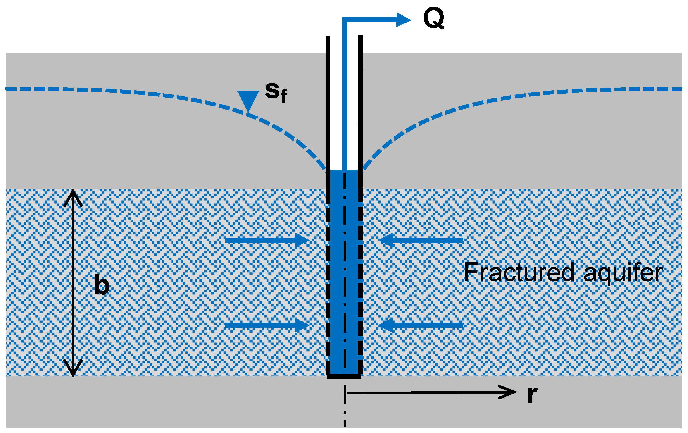
Consider a confined, fractured aquifer, horizontal and infinite in extent with a uniform thickness, as shown schematically in Figure 1.

Groundwater flow to a fully penetrating well is considered n-dimensional as described by Barker [13]

$$S_{sf}\frac{\partial s_f\left(r,t\right)}{\partial t}=\frac{K_f}{r^{n-1}}\frac{\partial }{\partial r}\left[r^{n-1}\frac{\partial s_f\left(r,t\right)}{\partial r}\right]-q\left(r,t\right),$$

(1)

where $s_f$ is the drawdown in the fractures [L], $S_{sf}$ is the specific storage of the fractures [L⁻¹], $K_f$ is the hydraulic conductivity of the fractures [L·T⁻¹], $q$ is the discharge from the matrix to the fractures per unit volume [T⁻¹], $r$ is the radial distance measured from the center of the well [L] and $t$ is the time since pumping started [T]. The initial condition is zero drawdown

$$s_f\left(r,0\right) =0,$$

(2)

and the boundary conditions are zero drawdown infinitely far from the well

$$s_f\left(\infty ,t\right) =0,$$

(3)

and a uniform constant pumping rate, taken in the limit for the well radius going to zero, and ignoring wellbore skin and storage effects

$$\underset{r\to 0}{\lim }\left[r^{n-1}\frac{\partial s_f\left(r,t\right)}{\partial r}\right] =-\frac{Q}{{\alpha }_n{K}_f{b}^{3-n}},$$

(4)

where $Q$ is the pumping rate [L³·T⁻¹], ${\alpha }_n$ is the area of a unit sphere in $n$ dimensions [-] and $b$ is the extent of the flow region [L] [13].

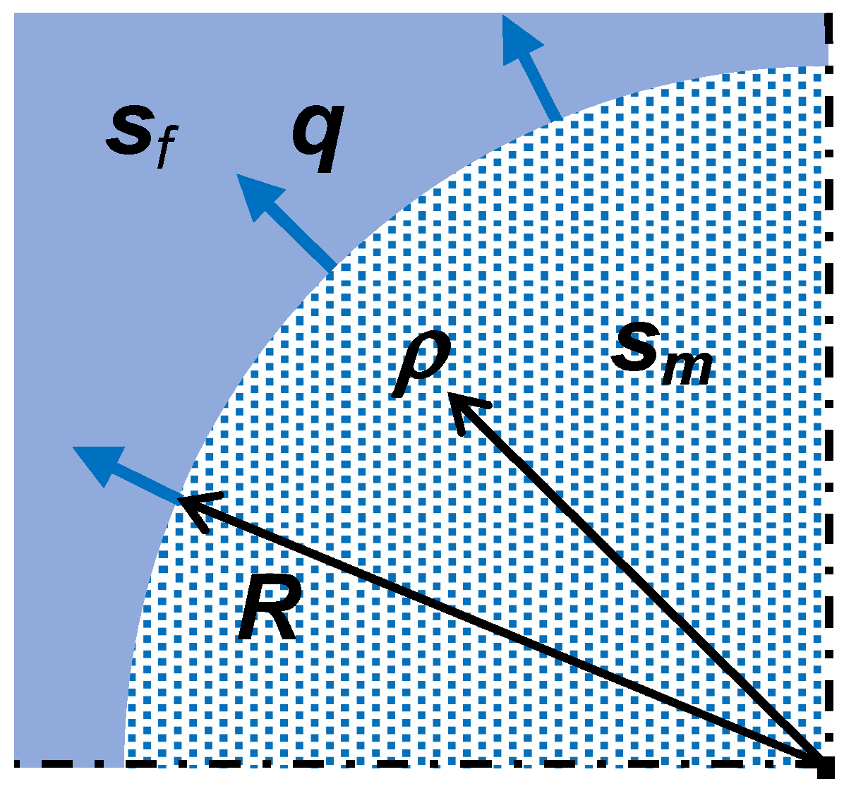
Exchange between matrix blocks and fractures is considered to be governed by $k$-dimensional diffusive transport in hyperspherical matrix blocks (Figure 2)

$$S_{sm}\frac{\partial s_m\left(r,\rho ,t\right)}{\partial t}=\frac{K_m}{{\rho }^{k-1}}\frac{\partial }{\partial \rho }\left[{\rho }^{k-1}\frac{\partial s_m\left(r,\rho ,t\right)}{\partial \rho }\right],$$

(5)

where $s_m$ is the drawdown in a matrix block [L], $S_{sm}$ is the specific storage of the matrix [L⁻¹], $K_m$ is the hydraulic conductivity of the matrix [L·T⁻¹] and $\rho$ is the radial coordinate of a $k$-dimensional spherical matrix block [L]. In case $k=1$ matrix blocks are infinite slabs, $k=2$ indicates infinite cylinders and $k=3$ spherical matrix blocks; non-integer values can be thought of as forms of matrix blocks that lie between slabs and cylinders (1 < k < 2) or between cylinders and spheres (2 < k < 3).

The initial condition in the matrix blocks is zero drawdown

$$s_m\left(r,\rho ,0\right) =0,$$

(6)

and the boundary conditions are symmetry at the origin (center of the matrix blocks)

$$\frac{\partial s_m\left(r,0,t\right)}{\partial \rho }=0,$$

(7)

and continuity at the interface with the fractures

$$s_m\left(r,R,t\right) =s_f\left(r,t\right),$$

(8)

where $R$ is the radius of the $k$-dimensional hyper-spherical matrix blocks [L]. Transport from the matrix to the fractures is obtained as

$$q\left(r,t\right) =-\frac{k{K}_m}{R}\frac{\partial s_m\left(r,R,t\right)}{\partial \rho },$$

(9)

where $k/R$ is the ratio between area and volume of a matrix block [L⁻¹].

3. Results

3.1. Analytical Solution

The solution is obtained by taking Laplace transforms; Barker [13] derived the solution in the Laplace domain as

$$\begin{array}{c}\mathcal{L}\left\{s_f\left(r,t\right);t\to p\right\} ={\tilde{s}}_f\left(r,p\right) =\frac{Q{r}^{\nu }{\mathrm{K}}_{\nu }\left(\lambda r\right)}{p{\alpha }_n{K}_f{b}^{3-n}{2}^{-\nu }\mathsf{\Gamma }\left(1-\nu \right){\lambda }^{\nu }}\\ \lambda =\sqrt{\frac{S_{sf}}{K_f}\left(p+k\frac{S_{sm}}{S_{sf}}\sqrt{\frac{p}{t_m}}\frac{{\mathrm{I}}_{\mu }\left(\sqrt{p{t}_m}\right)}{{\mathrm{I}}_{\mu -1}\left(\sqrt{p{t}_m}\right)}\right)}\end{array},$$

(10)

where $\mathcal{L}$ is the Laplace transform operator, $p$ is the Laplace transform variable [T⁻¹], $\widetilde{ }$ denotes a Laplace transformed variable, ${\mathrm{K}}_{\nu }$ and ${\mathrm{I}}_{\mu }$ are modified Bessel functions, $\nu =1-n/2$, $\mu =k/2$, $\mathsf{\Gamma }$ is the gamma function and $t_m=S_{sm}{R}^2/K_m$ is the characteristic time of transfer in the matrix blocks [T] (adapted after Barker [11]).

The convolution theorem of the iterated Laplace transform is used to derive the inverse Laplace transform [19] (p. 228)

$$\mathcal{L}\left\{{{\displaystyle \int }}_0^{t}f\left(\tau ,t-\tau \right)d\tau ;t\to p\right\} =\mathcal{L}\left\{\mathcal{L}\left\{f\left(t_1,t_2\right);t_1\to p\right\};t_2\to p\right\}.$$

(11)

Equation (10) is inverted in two steps by writing it as

$$\begin{array}{c}{\tilde{s}}_f\left(r,p_1,p_2\right) =\frac{Q{r}^{\nu }{\mathrm{K}}_{\nu }\left(\lambda r\right)}{p_2{\alpha }_n{K}_f{b}^{3-n}{2}^{-\nu }\mathsf{\Gamma }\left(1-\nu \right){\lambda }^{\nu }}\\ \lambda =\sqrt{\frac{S_{sf}}{K_f}\left(p_1+k\frac{S_{sm}}{S_{sf}}\sqrt{\frac{p_2}{t_m}}\frac{{\mathrm{I}}_{\mu }\left(\sqrt{p_2{t}_m}\right)}{{\mathrm{I}}_{\mu -1}\left(\sqrt{p_2{t}_m}\right)}\right)}\end{array}.$$

(12)

First it is inverted with respect to $p_1\to t_1$

$$\begin{array}{c}{\mathcal{L}}^{-1}\left\{{\tilde{s}}_f\left(r,p_1,p_2\right);p_1\to t_1\right\} =\frac{Q{r}^{2\nu }}{p_{2}4{\pi }^{1-\nu }{K}_f{b}^{3-n}{t}_1}{\left(\frac{S_{sf}{r}^2}{4K_f{t}_1}\right)}^{-\nu }\exp \left(\frac{-S_{sf}{r}^2}{4K_f{t}_1}\right)\times \\ \exp \left(-k\frac{S_{sm}}{S_{sf}}\frac{t_1}{t_m}\frac{\sqrt{p_2{t}_m} {\mathrm{I}}_{\mu }\left(\sqrt{p_2{t}_m}\right)}{{\mathrm{I}}_{\mu -1}\left(\sqrt{p_2{t}_m}\right)}\right),\end{array}$$

(13)

and next with respect to $p_2\to t_2$

$$\begin{array}{c}{\mathcal{L}}^{-1}\left\{{\mathcal{L}}^{-1}\left\{{\tilde{s}}_f\left(r,p_1,p_2\right);p_1\to t_1\right\};p_2\to t_2\right\} =\frac{Q{r}^{2\nu }}{4{\pi }^{1-\nu }{K}_f{b}^{3-n}{t}_1}{\left(\frac{S_{sf}{r}^2}{4K_f{t}_1}\right)}^{-\nu }\exp \left(\frac{-S_{sf}{r}^2}{4K_f{t}_1}\right)\times \\ {\mathcal{L}}^{-1}\left\{\frac{1}{p_2}\exp \left(-k\frac{S_{sm}}{S_{sf}}\frac{t_1}{t_m}\frac{\sqrt{p_2{t}_m} {\mathrm{I}}_{\mu }\left(\sqrt{p_2{t}_m}\right)}{{\mathrm{I}}_{\mu -1}\left(\sqrt{p_2{t}_m}\right)}\right);p_2\to t_2\right\},\end{array}$$

(14)

which, given Equation (11), leads to the following solution

$$s_f\left(r,t\right) =\frac{Q{r}^{2\nu }}{4{\pi }^{1-\nu }{K}_f{b}^{3-n}}{{\displaystyle \int }}_0^t{\left(\frac{S_{sf}{r}^2}{4K_f\tau }\right)}^{-\nu }\exp \left(\frac{-S_{sf}{r}^2}{4K_f\tau }\right)F_k\left[\frac{k{S}_{sm}\tau }{S_{sf}{t}_m},\frac{t-\tau }{t_m}\right]\frac{\mathrm{d}\tau }{\tau },$$

(15)

where

$$F_k\left(x,y\right) ={\mathcal{L}}^{-1}\left\{\frac{1}{p}\exp \left(-x\frac{\sqrt{p}{ \mathrm{I}}_{\mu }\left(\sqrt{p}\right)}{{\mathrm{I}}_{\mu -1}\left(\sqrt{p}\right)}\right);p\to y\right\}.$$

(16)

The solution in the form of a dimensionless well function is presented in Appendix A.

The inverse Laplace transform in Equation (16) is obtained by using an inversion theorem for the Fourier cosine transform [20] (Equation (1.6)). The derivation is lengthy but straightforward and yields

$$\begin{array}{c}{F}_k\left(x,y\right) =\frac{4}{\pi }{{\displaystyle \int }}_0^{\infty }\exp \left[-x\left(f_1+f_2\right)\right]\cos \left[x\left(f_1-f_2\right)\right]\sin \left(y{\lambda }^2\right){\lambda }^{-1}\mathrm{d}\lambda \\ f_1=\frac{\lambda }{\sqrt{2}}\left[\frac{{\mathrm{bei}}_{\mu }\left(\lambda \right){\mathrm{ber}}_{\mu -1}\left(\lambda \right)-{\mathrm{ber}}_{\mu }\left(\lambda \right){\mathrm{bei}}_{\mu -1}\left(\lambda \right)}{{\mathrm{ber}}_{\mu -1}^2\left(\lambda \right)+{\mathrm{bei}}_{\mu -1}^2\left(\lambda \right)}\right]\\ f_2=\frac{\lambda }{\sqrt{2}}\left[\frac{{\mathrm{ber}}_{\mu }\left(\lambda \right){\mathrm{ber}}_{\mu -1}\left(\lambda \right)+{\mathrm{bei}}_{\mu }\left(\lambda \right){\mathrm{bei}}_{\mu -1}\left(\lambda \right)}{{\mathrm{ber}}_{\mu -1}^2\left(\lambda \right)+{\mathrm{bei}}_{\mu -1}^2\left(\lambda \right)}\right]\end{array},$$

(17)

where ${\mathrm{ber}}_{\mu }$ and ${\mathrm{bei}}_{\mu }$ are Kelvin functions. Equation (17) can be simplified in case $k=1$ (slab matrix blocks) as

$$\begin{array}{c}{f}_1=\frac{\lambda }{\sqrt{2}}\left[\frac{\sinh \left(\sqrt{2}\lambda \right)}{\cosh \left(\sqrt{2}\lambda \right)+\cos \left(\sqrt{2}\lambda \right)}\right]\\ f_2=-\frac{\lambda }{\sqrt{2}}\left[\frac{\sin \left(\sqrt{2}\lambda \right)}{\cosh \left(\sqrt{2}\lambda \right)+\cos \left(\sqrt{2}\lambda \right)}\right]\end{array},$$

(18)

or in case $k=3$ (spherical matrix blocks) as

$$\begin{array}{c}{f}_1=\frac{\lambda }{\sqrt{2}}\left[\frac{\sinh \left(\sqrt{2}\lambda \right)}{\cosh \left(\sqrt{2}\lambda \right)-\cos \left(\sqrt{2}\lambda \right)}\right]-\frac{1}{2}\\ f_2=\frac{\lambda }{\sqrt{2}}\left[\frac{\sin \left(\sqrt{2}\lambda \right)}{\cosh \left(\sqrt{2}\lambda \right)-\cos \left(\sqrt{2}\lambda \right)}\right]-\frac{1}{2}\end{array}.$$

(19)

3.2. Approximations for Small and Large Times

The application of the solution given by Equations (15) and (17) can be cumbersome in practice, depending on the capabilities of the user. Therefore, we also present approximations for small and large times that are much easier to apply.

A small time implies $p\to \infty$ or $\sqrt{p}{\mathrm{I}}_{\mu }\left(\sqrt{p}\right)/{\mathrm{I}}_{\mu -1}\left(\sqrt{p}\right) \approx \sqrt{p}-\left(\mu -\frac{1}{2}\right)$, so that Equation (16) can be approximated as

$$F_k\left(x,y\right) \approx {\mathcal{L}}^{-1}\{p^{-1}\exp (-x\sqrt{p}+\frac{1}{2}\left(k-1\right)x);p\to y\},$$

(20)

which can be inverted as

$$F_k\left(x,y\right) \approx \exp \left[\frac{1}{2}\left(k-1\right)x\right]\mathrm{erfc}\left[\frac{x}{2\sqrt{y}}\right],$$

(21)

where erfc is the complementary error function. When Equation (21) is inserted in Equation (15), we obtain an approximate solution for small times. In case of cylindrical flow to the well ($n=2$) and slab matrix blocks ($k=1$), the small-time approximation becomes

$$s_f\left(r,t\right) \approx \frac{Q}{4\pi K_{f}b}{{\displaystyle \int }}_0^t\exp \left(\frac{-S_{sf}{r}^2}{4K_f\tau }\right)\mathrm{erfc}\left(\frac{S_{sm}}{2S_{sf}\sqrt{t_m}}\frac{\tau }{\sqrt{t-\tau }}\right)\frac{\mathrm{d}\tau }{\tau },$$

(22)

which is mathematically equivalent to the solution of Hantush [21] for well flow in a leaky aquifer with storage released from an infinitely thick aquitard.

Large time implies $p\to 0$ or $\sqrt{p}{\mathrm{I}}_{\mu }\left(\sqrt{p}\right)/{\mathrm{I}}_{\mu -1}\left(\sqrt{p}\right) \approx \left(k+2\right)p/\left[k\left(k+2\right)+p\right]$, so that Equation (16) can be approximated as

$$F_k\left(x,y\right) \approx {\mathcal{L}}^{-1}\left\{p^{-1}\exp \left(-x\frac{\left(k+2\right)p}{k\left(k+2\right)+p}\right);p\to y\right\},$$

(23)

which can be inverted as

$$F_k\left(x,y\right) \approx \mathrm{J}\left[\left(k+2\right)x,k\left(k+2\right)y\right],$$

(24)

where J is the Bessel integral [3,22]. When this equation is inserted in Equation (15), we obtain an approximate solution for large times. In case of cylindrical flow to the well ($n=2$), the large-time approximation becomes

$$s_f\left(r,t\right) \approx \frac{Q}{4\pi K_{f}b}{{\displaystyle \int }}_0^t\exp \left(\frac{-S_{sf}{r}^2}{4K_f\tau }\right)\mathrm{J}\left[\frac{k\left(k+2\right)S_{sm}\tau }{S_{sf}{t}_m},\frac{k\left(k+2\right)\left(t-\tau \right)}{t_m}\right]\frac{\mathrm{d}\tau }{\tau },$$

(25)

which is mathematically equivalent to the solution of De Smedt [3] for well flow in a double-porosity aquifer with steady state exchange between matrix and fractures. The similarity between transient and steady state exchange for large times has also been reported in other studies, e.g., [12]. Because $p\to 0$ implies $y\to \infty$, Equation (24) can be further simplified by an asymptotic expansion adapted from Goldstein [22] as

$$F_k\left(x,y\right) \approx \frac{1}{2} \mathrm{erfc}\left\{\sqrt{\left(k+2\right)x}-\sqrt{k\left(k+2\right)y}-\frac{1}{4}{\left[k{\left(k+2\right)}^{2}xy)\right]}^{-1/4}\right\}.$$

(26)

4. Discussion

The solution presented in this study extends the work of previous studies by deriving an analytical solution for groundwater flow to a pumping well in a fractured aquifer with transient exchange between matrix blocks and fractures. The solution is mainly based on the work of Baker [13] who introduced fractional flow dimensions but used the numerical inversion of a semi-analytical solution in the Laplace domain. The current solution differs from other approaches such as Moench [8], Baker [11,12], Hamm and Bidaux [14], Lods and Gouze [15], Dejam et al. [17] and Sedghi and Samani [18], which presented semi-analytical solutions, while the current fully analytic solution is theoretically more attractive and gives the user more flexibility to compute and apply in practice. The analytical solution also differs from other analytical solutions as presented by Boulton and Streltsova [5], Swaan [9] and Bourdet and Gringarten [6], in that it is more general because it takes into account different and intermediate shapes of matrix blocks and different and fractional flow dimensions. Moreover, the derived asymptotic approximations for small and large times are new, original contributions that are easy to compute and apply in practice.

The practical application of the model, given by Equations (15) and (17), requires some arithmetic skills of the user and/or the availability of appropriate numerical codes to evaluate the integrals and special functions that appears in the equations. In particular, the improper integral in Equation (17) must be computed with some care due to the oscillating nature of the trigonometric functions in the integrand. However, the integral in Equation (15) is definite, while the improper integral in Equation (17) has an integrand that tends to zero quickly because of the negative argument in the exponential term. Alternatively, one can also use Equation (15) in combination with Equation (16) and the numerical inversion of the Laplace transform for the latter. On the other hand, the approximate solutions for small and large times, given by Equations (15), (21) and (26), contain only definite integrals with integrands consisting of well-known and easily computable continuous functions.

The analytical solution can be used to analyze pumping tests and estimate aquifer parameters considering the following assumptions:

• The aquifer is homogeneous, isotropic and confined.
• The aquifer is infinite in horizontal extent with uniform thickness.
• The aquifer consists of fractures and matrix blocks; flow mainly takes place in the fractures and water storage mainly in the matrix blocks.
• The flow in the aquifer is described by Darcy’s law.
• The well fully penetrates the aquifer and has an infinitely small diameter; well-bore storage and skin effects are negligible.
• The well is pumped at a constant rate.

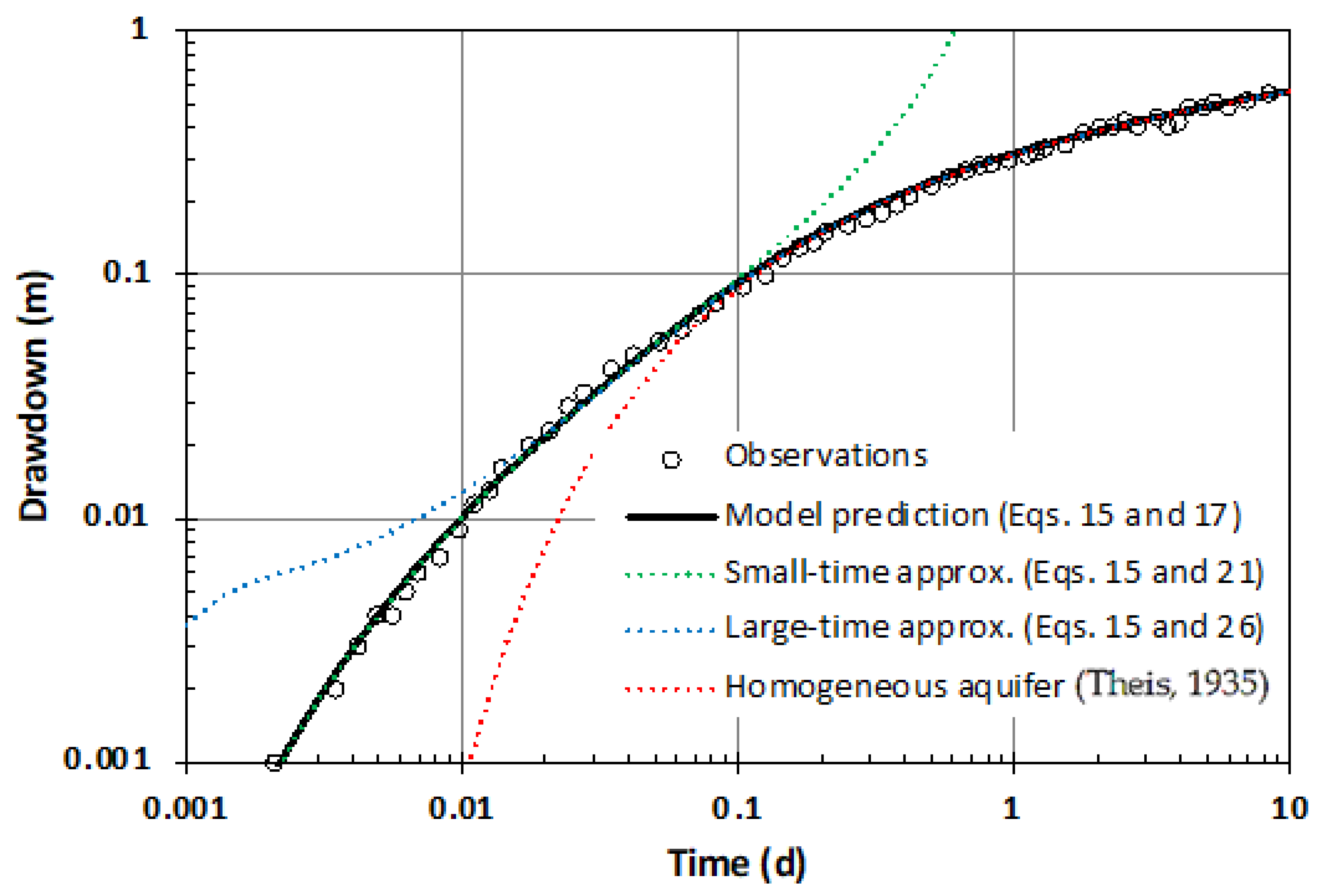
In order to facilitate the discussion, the solution is applied to a field example presented by Nielsen [23]. The pumping test was performed in a fractured chalk aquifer in central Sjælland, Denmark and lasted for about 8 days. The pumping rate was 1836 m³/d and drawdown was recorded in an observation well at a distance of 1213 m from the pumping well. The pumping well and monitoring well fully penetrate the aquifer to a depth of about 60 m. The chalk layer has a thickness of about 40 m and is confined by an overlying clay layer of about 20 m thickness. Observed drawdown, shown in Figure 3, ranged from 1 mm to 0.55 m. Although the variation was quite smooth, the observations cannot be fitted with a Theis well function [24] as shown by the solid red curve in Figure 3, indicating that the aquifer did not respond to well flow as a homogenous porous medium.

The solution given by Equations (15) and (17) depends on six parameters: $K_f$ the hydraulic conductivity of the fractures, $S_{sf}$ the specific storage of the fractures, $n$ the well flow dimensions, $t_m$ the characteristic time of transfer in the matrix blocks, $S_{sm}$ the specific storage of the matrix and $k$ the dimensions of the interactive flow from the matrix blocks to the fractures. However, it is impossible to estimate all six parameters with confidence because the observations are too limited as there are only 56 drawdown observations were obtained in a single observation well. If more observation wells with large series of accurate drawdown recordings were available, more parameters could likely be estimated, but we have not been able to find such data in the literature. Therefore, in this case, some parameters should be determined by expert opinion. We chose to apply two-dimensional cylindrical flow to the well (n = 2) and three-dimensional spherical flow in the matrix blocks (k = 3). The analytical solution is coupled with a parameter optimization algorithm and the remaining parameters are estimated to obtain the best match between observed and simulated drawdowns by minimizing the sum of squared residuals between the observations and model predictions. To give equal importance to small drawdown values at the beginning of the pumping test as to larger values at the end, logarithms of the observations are used in the fitting procedure. The results are shown in

Table 1. Model optimization results for the pumping test performed in a fractured chalk aquifer in central Sjælland, Denmark [22]; given are mean fitted aquifer parameter values, 95 % confidence intervals (CI) of the estimated parameter values and Student’s t-test (t-value) which should be larger than 1.96 to be significant.

Parameter	Estimate	± 95% CI	t-Value
$K_f$ (m2/d)	32.8	1.7	39.4
$S_{sf}$ (m−1)	1.38 × 10−7	0.57 × 10−7	4.9
$t_m$ (d)	0.189	0.051	7.4
$S_{sm}$ (m−1)	2.98 × 10−6	0.21 × 10−6	28.9

. Given in the table are estimated values of the model parameters, ±95% confidence intervals of the estimates and the corresponding Student’s t-test value. All estimated values for the aquifer parameters are relevant and acceptable from a physical point of view. The t-values also show that all parameters are estimated with confidence (t-value > 1.96). In particular, the hydraulic conductivity of the fractures and the specific storage of the matrix are estimated with large confidence; these are usually the most important aquifer parameters that one wants to identify for groundwater management or groundwater flow modelling. Note also that it is possible to estimate the hydraulic conductivity of the matrix if the size of the matrix blocks is known ($K_m=S_{sm}{R}^2/t_m$). For example, assuming spherical matrix blocks with a radius of 0.2 m, this would give a hydraulic conductivity of the matrix of 6.2 × 10⁻⁵ m·d⁻¹.

The predicted drawdown in the fractures is represented by the black line in Figure 3 (note that the curve is completely covered by the other curves) and the fit with the observations appears to be very good. These results are also verified by numerical inversion of the solution in the Laplace domain given by Equation (10); differences with the analytical solution are less than 10⁻⁴.

The drawdown predicted by the approximate solution for small times, given by Equations (15) and (21), is shown in Figure 3 by the green line, which closely matches the observations and completely overlaps the full analytical solution for small times. The drawdown predicted by the approximate solution for large times, given by Equations (15) and (26), is shown in Figure 3 by the blue line, which closely matches the observations and completely overlaps the full analytical solution for large times. Note that it is possible to describe the drawdown for all times by combining the small-time and large-time approximations, which are easy to calculate in practice. A suitable break point between the small-time and large-time approximations is given by $t=t_m/3$. The differences with the full solution are less than 10⁻⁵.

If the aquifer were a single porosity system with the storage capacity of the fractures and matrix combined, the drawdown over time would follow a Theis curve [24] in case of cylindrical flow to the well (n = 2) as shown by the red line in Figure 3, which only matches the observations for very large times, as expected for double-porosity media.

5. Conclusions

An analytical solution for well flow in fractured porous media was presented based on the double-porosity approach with transient exchange between fractures and matrix. The solution takes into account fractional flow dimensions including linear, cylindrical or spherical flow to the well and fractional inter-porosity transfer dimensions including release from storage in infinite slabs, infinite cylinders or spherical matrix blocks.

The usefulness of the model was demonstrated with a practical example consisting of a pumping test performed in a fractured chalk aquifer. The results show that all observations can be reproduced very well by the model with estimated parameter values that are physically relevant and statistically reliable. It was also shown how this solution compares to other pumping test solutions, such as the Theis and Hantush well functions and the solution for well flow in double-porosity media assuming steady state exchange between matrix and fractures. Small-time and large-time approximations were presented that are easy to apply in practice. Therefore, this study provides new and practical tools for analyzing pumping tests in fractured porous media characterized by double-porosity effects.

The analytical solution does not account for wellbore storage and skin effects and therefore cannot be applied to analyze drawdown in the well or close to the well until wellbore storage and skin effects become insignificant.

References

- Barenblatt, G.I.; Zheltov, I.P.; Kochina, I.N. Basic concepts in the theory of seepage of homogeneous liquids in fissured rocks [strata]. J. Appl. Math. Mech. 1960, 24, 1286–1303. [Google Scholar] [CrossRef]
- Warren, J.E.; Root, P.J. The behavior of naturally fractured reservoirs. Soc. Pet. Eng. J. 1963, 3, 245–255. [Google Scholar] [CrossRef] [Green Version]
- De Smedt, F. Analytical solution for constant-rate pumping test in fissured porous media with double-porosity behaviour. Transp. Porous Media 2011, 88, 479–489. [Google Scholar] [CrossRef]
- Kazemi, H. Pressure transient analysis of naturally fractured reservoirs with uniform fracture distribution. Soc. Pet. Eng. J. 1969, 9, 451–462. [Google Scholar] [CrossRef]
- Boulton, N.S.; Streltsova, T.D. Unsteady flow to a pumped well in a fissured water-bearing formation. J. Hydrol. 1977, 35, 257–269. [Google Scholar] [CrossRef]
- Bourdet, D.; Gringarten, A.C. Determination of fissure volume and block size in fractured reservoirs by type-curve analysis. In Proceedings of the SPE Annual Technical Conference and Exhibition, Dallas, TX, USA, 21–24 September 1980. [Google Scholar] [CrossRef]
- Streltsova, T.D. Hydrodynamics of groundwater flow in a fractured formation. Water Resour. Res. 1976, 12, 405–414. [Google Scholar] [CrossRef]
- Moench, A.F. Double-porosity models for a fissured groundwater reservoir with fracture skin. Water Resour. Res. 1984, 20, 831–846. [Google Scholar] [CrossRef]
- De Swaan, A. Analytic solutions for determining naturally fractured reservoir properties by well testing. Soc. Pet. Eng. J. 1876, 16, 117–122. [Google Scholar] [CrossRef] [Green Version]
- Barker, J.A.; Black, J.H. Slug tests in fissured aquifers. Water Resour. Res. 1983, 19, 1558–1564. [Google Scholar] [CrossRef]
- Barker, J.A. Generalized well function evaluation for homogeneous and fissured aquifers. J. Hydrol. 1985, 76, 143–154. [Google Scholar] [CrossRef]
- Barker, J.A. Block-geometry functions characterizing transport in densely fissured media. J. Hydrol. 1985, 77, 263–279. [Google Scholar] [CrossRef]
- Barker, J.A. A generalized radial flow model for hydraulic tests in fractured rock. Water Resour. Res. 1988, 24, 1796–1804. [Google Scholar] [CrossRef] [Green Version]
- Hamm, S.; Bidaux, P. Dual-porosity fractal models for transient flow analysis in fissured rocks. Water Resour. Res. 1996, 32, 2733–2745. [Google Scholar] [CrossRef]
- Lods, G.; Gouze, P. WTFM, Software for well test analysis in fractured media combining fractional flow with double porosity and leakance approaches. Comput. Geosci. 2004, 30, 937–947. [Google Scholar] [CrossRef]
- Lods, G.; Gouze, P. A generalized solution for transient radial flow in hierarchical multifractal fractured aquifers. Water Resour. Res. 2008, 44, W12405. [Google Scholar] [CrossRef]
- Dejam, M.; Hassanzadeh, H.; Chen, Z. Semi-Analytical solutions for a partially penetrated well with wellbore storage and skin effects in a double-porosity system with a gas cap. Transp. Porous Media 2013, 100, 159–192. [Google Scholar] [CrossRef]
- Sedghi, M.M.; Samani, N. Semi-analytical solutions for flow to a well in an unconfined-fractured aquifer system. Adv. Water Resour. 2015, 83, 89–101. [Google Scholar] [CrossRef]
- Sneddon, I.N. The Use of Integral Transforms; Tata McGraw-Hill Publishing, Co. Ltd.: Noida, India, 1974. [Google Scholar]
- Davies, B.; Martin, B. Numerical inversion of the Laplace transform: A survey and comparison of methods. J. Comput. Phys. 1979, 33, 1–32. [Google Scholar] [CrossRef]
- Hantush, M.S. Hydraulics of wells. Adv. Hydrosci. 1964, 1, 281–432. [Google Scholar] [CrossRef]
- Goldstein, F.R.S. On the mathematics of exchange processes in fixed columns I: Mathematical solutions and asymptotic expansions. Proc. R. Soc. Lond. 1953, 219, 151–185. [Google Scholar] [CrossRef]
- Nielsen, K.A. Fractured Aquifers—Formation Evaluation by Well Testing; Trafford Publishing: Victoria, BC, Canada, 2007. [Google Scholar]
- Theis, C.V. The relation between the lowering of the piezometric surface and the rate and duration of discharge of a well using groundwater storage. Eos Trans. Am. Geophys. Union 1935, 16, 519–524. [Google Scholar] [CrossRef]
Figure 1.
Schematic cross-section of groundwater flow to a well in a fractured aquifer.
Figure 2.
Schematic cross-section of groundwater flow from matrix blocks to fractures.
Figure 3.
Results of the pumping test analysis showing the drawdown in the fractures over time; given are: observed values, model predictions (Equations (15) and (17)), small-time approximation (Equations (15) and (21)), large-time approximation (Equations (15) and (26)), and in case the aquifer is homogeneous (Theis [24]). Note that the black curve is completely covered by the other curves.