Article

Assessing Performances of Multivariate Data Assimilation Algorithms with SMOS, SMAP, and GRACE Observations for Improved Soil Moisture and Groundwater Analyses

by
Natthachet Tangdamrongsub
1,2,*,
Jianzhi Dong
3 and
Peter Shellito
4
1
Earth System Science Interdisciplinary Center, University of Maryland, College Park, MD 20742, USA
2
Hydrological Sciences Laboratory, NASA Goddard Space Flight Center, Greenbelt, MD 20771, USA
3
Department of Civil and Environmental Engineering, Massachusetts Institute of Technology, Cambridge, MA 02139, USA
4
Oxbow Science, LLC, Seattle, WA 98103, USA
*
Author to whom correspondence should be addressed.
Submission received: 30 December 2021 / Revised: 14 February 2022 / Accepted: 15 February 2022 / Published: 17 February 2022
(This article belongs to the Special Issue Remote Sensing for Water Storage and Soil Moisture Estimates)

Abstract

:
Multivariate data assimilation (DA) of satellite soil moisture (SM) and terrestrial water storage (TWS) observations has recently been used to improve SM and groundwater storage (GWS) simulations. Previous studies employed the ensemble Kalman approach in multivariate DA schemes, which assumes that model and observation errors have a Gaussian distribution. Despite the success of the Kalman approaches, SM and GWS estimates can be suboptimal when the Gaussian assumption is violated. Other DA approaches, such as particle smoother (PS), ensemble Gaussian particle smoother (EnGPS), and evolutionary smoother (EvS), do not rely on the Gaussian assumption and may be better suited to non-Gaussian error systems. The objective of this paper is to evaluate the performance of these four DA approaches (EnKS, PS, EnGPS, and EvS) in multivariate DA systems by assimilating satellite data from the Soil Moisture and Ocean Salinity (SMOS), Soil Moisture Active Passive (SMAP), and Gravity Recovery And Climate Experiment (GRACE) missions into the Community Atmosphere and Biosphere Land Exchange (CABLE) land surface model. The analyses are carried out in Australia’s Goulburn River catchment, where in situ SM and groundwater data are available to comprehensively validate the DA performance. Results show that all four DA approaches have outstanding performances and improve correlation coefficients of SM and GWS estimates by ~20% and 100%, respectively. The EvS outperforms the others, but its benefit is relatively marginal compared to Gaussian approaches (e.g., EnKS). This is due to the fact that SM and TWS error distributions in this study are close to Gaussian: a suitable condition for, e.g., EnKS, EnGPS. The robust performance of EvS appears to be the optimal approach for jointly assimilating multi-source hydrological observations to improve regional hydrological analyses.

1. Introduction

The accurate estimation of terrestrial water storage (TWS) is critical for regional water resource analyses. TWS can be calculated using a land surface model (LSM), which incorporates complex land–surface processes into simulations of a wide range of hydrologic variables [1]. However, the performance of LSMs is frequently constrained by factors such as insufficient model physics representation, simplified model parameters, or inaccurate meteorological forcing, resulting in significant uncertainty of simulation results [2]. Data assimilation (DA) is an important technique for correcting model state variables with satellite data, resulting in more robust hydrologic variables [3].
Advanced DA systems are capable of incorporating univariate and multivariate data into models. Univariate DA is an approach for updating model states using only one type of satellite observation [4]. Despite its success, univariate DA usually improves only one state variable associated with the assimilated observation, while the effect on other variables can be insignificant or negative. For example, Yan and Moradkhani [5] discovered that assimilating streamflow could lead to biased estimates of soil moisture (SM). Similarly, Tian et al. [6] reported a reduction in the accuracy of groundwater storage (GWS) estimates after assimilating satellite SM observations. Multivariate DA, as compared to univariate DA, uses a suite of satellite observations to simultaneously constrain multiple model states, resulting in a better overall representation of hydrologic systems [7,8].
Previous studies developed TWS/SM multivariate DA based on ensemble Kalman approaches such as ensemble Kalman filter (EnKF [9]) and ensemble Kalman smoother (EnKS [6,10]). Ensemble Kalman algorithms determine solutions based on random samples associated with Gaussian error distributions. Although EnKF and EnKS have been useful for many environmental modeling problems [11,12,13,14], they are potentially sub-optimal given that error distributions of models or measurements are mostly non-Gaussian [2,15]. DA approaches that are not restricted to specific error distributions, such as particle filters [16], might be more suitable for highly nonlinear systems. Such approaches also include an evolutionary DA that utilizes genetic algorithms to determine the optimal solution, i.e., through a natural selection process [17]. Because the evolutionary approach is based on an intrinsic error distribution (rather than a Gaussian distribution), it may result in better SM and TWS estimates. However, despite its success in improving evapotranspiration, soil moisture, and streamflow estimates, the evolutionary DA has yet to be implemented or investigated for multivariate SM/TWS estimations [18,19,20].
This study aims to assess the performance of four different DA algorithms on multivariate DA using satellite SM and TWS data. The DA approaches are (1) EnKS, (2) particle smoother (PS [21]), and for the first time, (3) an ensemble Gaussian particle smoother (EnGPS) and (4) evolutionary smoother (EvS). The satellite SM and TWS observations are simultaneously assimilated into the Community Atmosphere and Biosphere Land Exchange (CABLE) LSM [22,23] with the purpose of improving regional SM and GWS estimates. This assessment is conducted in the Goulburn River catchment in Australia, where in situ SM and groundwater level data are available for validation. The analysis period is between January 2010 and December 2015, when satellite and validation data are available. The findings of this study may shed some light on the selection and development of robust multivariate DA algorithms for improved regional terrestrial hydrology analyses.

2. Model, Study Area, and Data

2.1. Model Configurations

The CABLE LSM is used to simulate daily SM and GWS at 0.25° × 0.25° resolution. The CABLE model can be obtained from https://trac.nci.org.au/trac/cable (last access: 25 November 2021). This section describes the model configuration used in our analysis, and comprehensive model descriptions can be found in Decker [22]. CABLE estimates SM in six distinct layers. The soil thicknesses from top to bottom are set to 1.2, 3.8, 25, 39.9, 107.9, 287.2 cm, respectively. Together, the first two model soil layers correspond to the 0–5 cm sampling depth of in situ SM measurements and satellite SM estimates (see Section 2.2 and Section 2.3). The groundwater layer is defined as a 20 m thick unconfined aquifer located below the soil layers. The forcing data required for CABLE simulations are obtained from the Global Land Data Assimilation System (GLDAS [24]). GLDAS precipitation is replaced by data from the Integrated Multi-satellite Retrievals for Global Precipitation Measurement Mission (IMERG [25]) to improve the accuracy of TWS estimates [26].
In the DA process, the precipitation is perturbed by multiplicative white noise. The perturbation magnitude is obtained from the uncertainty provided by the IMERG product. Shortwave radiation is perturbed using multiplicative white noise at 10% of the nominal values. An additive white noise of 2 °C is used for the air temperature. Perturbations of the forcing data utilize an exponential correlation function to maintain spatial consistency: a 0.25° correlation length is applied to the covariance matrix for each forcing variable. Model parameters associated with SM and GWS components are also perturbed by 10% of their magnitudes. These parameters consist of the fractions of clay/sand/silt and the drainage parameters that control the soil storage capacity and subsurface runoff (see Table 1 in Tangdamrongsub et al. [10] for more details).

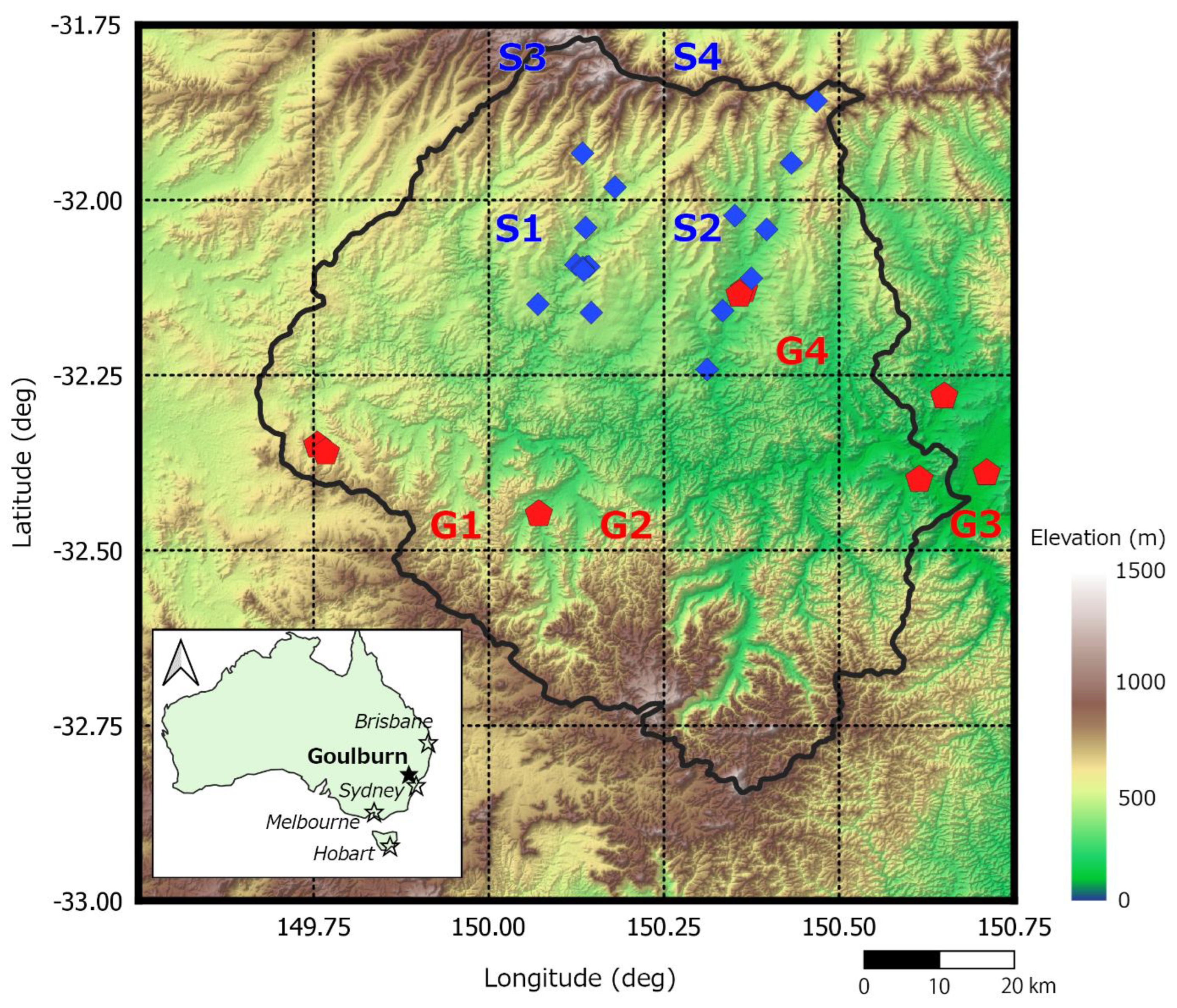
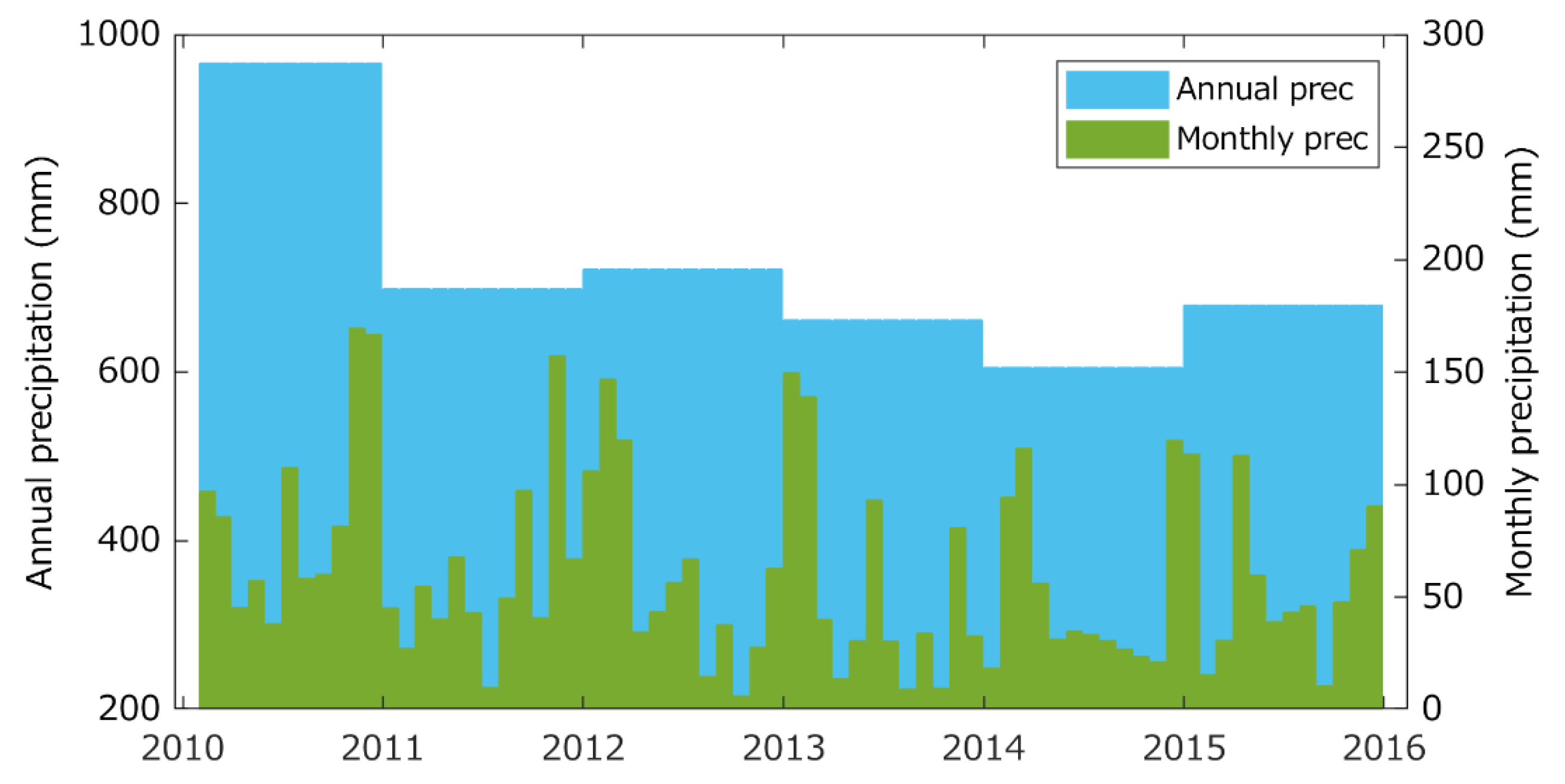
2.2. Study Area and In Situ Data

The Goulburn River catchment (6540 km2) is located in New South Wales, approximately 200 km northwest of Sydney (Figure 1). In the north, the catchment consists of a floodplain, clear grassland, and crops. In the south, there is a mountain range with dense vegetation. Summer average minimum/maximum temperatures in the catchment are 16/30 °C, and winter temperatures are 2/14 °C. As such, snowfall is scarce in the catchment area. The Scaling and Assimilation of Soil Moisture and Streamflow (SASMAS) project collects volumetric SM measurements at various sampling depths [27], and the 0–5 cm data are used in this study due to their compatibility with CABLE’s top two soil layers. The soil moisture profile is measured using water content reflectometers. Sensors were installed by excavating to the top of the sensor installation level and then backfilling to ensure continuous monitoring of the soil moisture profile. The accuracy of the in situ measurement is approximately 0.035 m3/m3, as determined by comparing probe data to independent gravimetric soil moisture samples. Comprehensive details of field measurements can be found in Rüdiger et al. [27]. In situ groundwater level (GWL) data are provided by the Department of Primary Industries (DPI), Office of Water, New South Wales (http://www.water.nsw.gov.au; last access: 23 December 2020). At each location, groundwater depth measurements are converted to groundwater depth variations by removing the long-term mean from all available data in the time series. Sites are excluded if the time series is shorter than three years or has significant data gaps. Prior to validation, the point measurements of in situ data inside the same model grid cell are averaged. This procedure is carried out to reduce the spatial resolution inconsistency between ground measurements and the model.

2.3. Satellite Soil Moisture Data

The daily satellite SM retrievals are obtained from Soil Moisture and Ocean Salinity (SMOS [28]) and Soil Moisture Active Passive (SMAP [29]). Both carry L-band (1.4 GHz) radiometers that are used to estimate 0–5 cm soil moisture. SMOS data are the Level 3 (Release 4) gridded product [30] provided by the Centre Aval de Traitement des Données SMOS (CATDS; https://www.catds.fr; last access: 23 December 2020) operated for the Centre National d’Etudes Spatiales (CNES) by the French Research Institute for Exploitation of the Sea (IFREMER). The product has a spatial resolution of ~25 km on the Equal-Area Scalable Earth (EASE) grid and is available from 15 January 2010. SMAP data are the Level 3 Radiometer Global Daily 36 km EASE-Grid Soil Moisture Version 6 provided by the National Snow and Ice Data Center Distributed Active Archive Center (NSIDC DAAC; https://nsidc.org/data/smap; last access: 23 December 2020). The product provides a composite of daily SM and is available from 31 March 2015. For spatial consistency with the model, both SMOS and SMAP data are resampled to a 0.25° × 0.25° regular grid using a nearest neighbor interpolation method. When more than one SM retrieval is available on a given day, the average value is used to ensure temporal consistency with the model.
Assimilating satellite SM data into LSMs requires rescaling to reduce systematic bias between model estimates and observations [31,32]. In this study, a cumulative density function matching approach (CDF-matching [32]) is used to adjust satellite observations to model climatology. The CDF is constructed using all the data in the study period, and the rescaling is applied separately for each satellite data product and individual model grid cell. Following previous studies, a 0.04 m3/m3 measurement error is used for both SMOS and SMAP data [33,34].

2.4. GRACE Data

This study uses GRACE mascons Release 6 Version 2 provided by the Center for Space Research (CSR) at the University of Texas Austin [35]. The data are obtained from http://www2.csr.utexas.edu/grace/RL06_mascons.html (last access: 23 December 2020). The mascon product contains monthly TWS variations at 0.25° grid size derived from GRACE [36] and GRACE Follow-On missions [37] from April 2002. It is noteworthy that mascons only use 0.25° grid size for properly rendering mass redistribution near coastal areas, whereas the native resolution of GRACE is approximately 3°. At each mascon cell, the long-term mean computed from all data between January 2010 and December 2015 is removed to obtain TWS variations relative to our analysis period.
Prior to the DA process, the long-term mean TWS (January 2010 and December 2015) from CABLE estimates is added to the GRACE-derived TWS variation to reduce systematic differences between observed and modeled mean TWS. The CSR product does not include observational errors, and the 2 cm TWS error proposed by [38] is used in this study. Additionally, spatial correlation errors are included when perturbing GRACE observations, given that the GRACE-derived TWS spatial resolution is on the order of 3°. The correlation error ( C ) is calculated as C = e x p ( ψ / L ) , where ψ is a spherical distance between two grid points, and L is the correlation length (3°).

3. Methodology

The concept of multivariate DA implementation is explained in this section. Table 1 summarizes the characteristics of the DA algorithms, while Appendix A, Appendix B, Appendix C and Appendix D provide detailed descriptions.

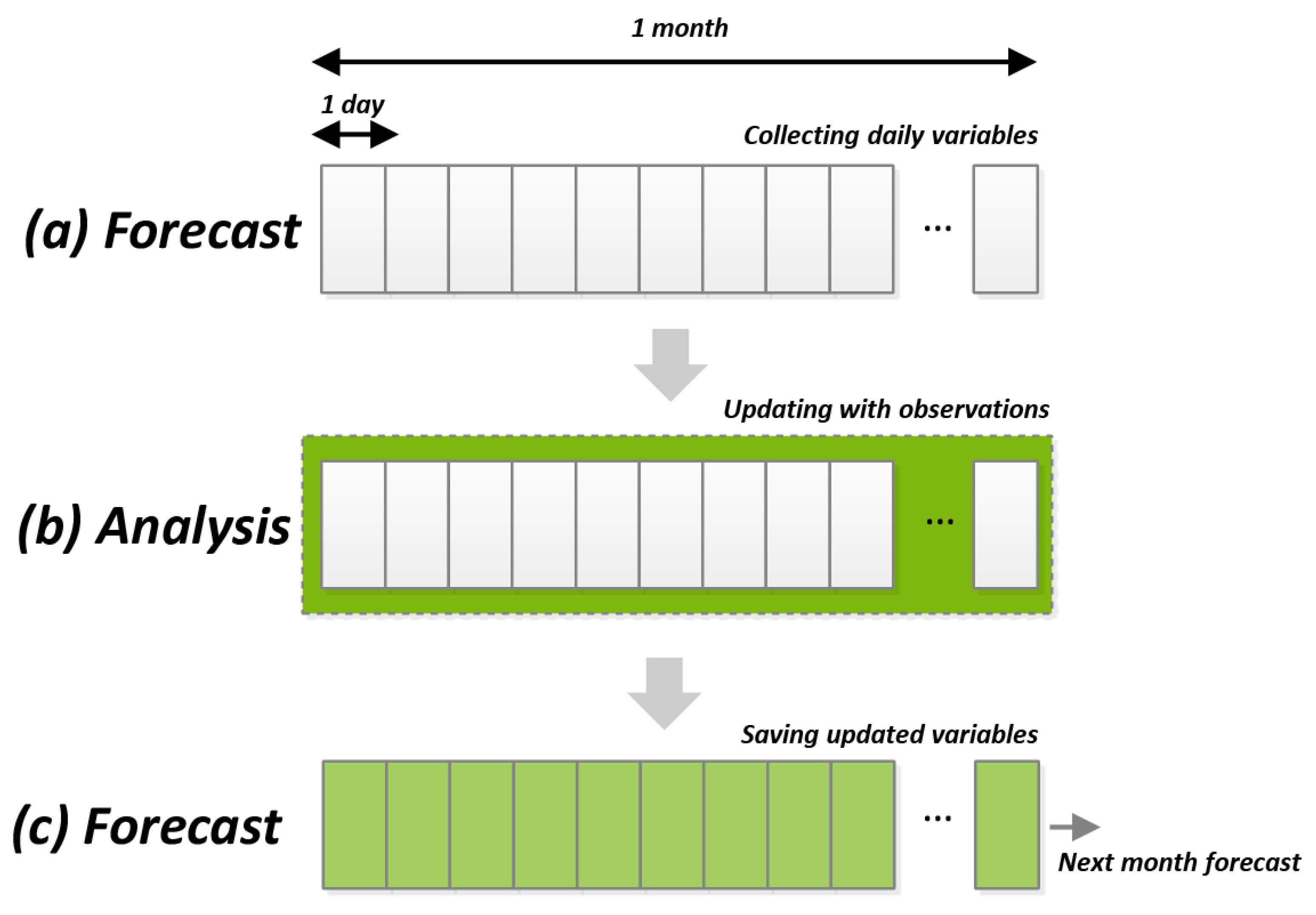
3.1. Implementation of Multivariate DA

This study assimilates SMOS, SMAP, and GRACE observations into CABLE using four different DA approaches, namely EnKS, PS, EnGPS, and EvS, and updates modeled SM and GWS estimates every month. The DA schematic is similar to that of Tangdamrongsub et al. [10], with a slight modification to the assimilated time widow. The DA process consists of forecast and analysis steps (Figure 2). In the forecast step, forcing data and model parameters are firstly perturbed using N ensemble members (N = 100 is used in this study). The model is then propagated for s days to forecast s-day state variables (i.e., SM and GWS):
x s | t 1 i = 𝓕 ( x t 1 i , f s i , α i )
where 𝓕 is a model operator used to propagate the states from t 1 (initial state) to s day forecast, x is a model state vector, f is forcing data, α is model parameters, and i denotes the index of the ensemble members. The initial states are obtained in the first step of simulations by spinning up the model between 2010 and 2015 for 10 revolutions, at which point all storage variables reach equilibrium states. The state vector comprises seven different variables: six SM layers and GWS. It should be noted that snow water equivalent and canopy storage are negligible in the Goulburn River catchment and are not included in the state vector. The forecasts can be converted to SM ( d s ( SM ) ) and TWS ( d s ( TWS ) ) values as follows:
d s ( SM ) i = H ( SM ) x s i
d s ( TWS ) i = H ( TWS ) x s i
where H is the operation matrix relating model state vectors to SM and TWS observational spaces. The H matrix has a dimension of s × 7s associated with s day forecast period and seven state variables:
H ( SM ) = [ 1   1   0   0   0   0   0 0   0   0   0   0   0   0 0   0   0   0   0   0   0 0   0   0   0   0   0   0 1   1   0   0   0   0   0 0   0   0   0   0   0   0 0   0   0   0   0   0   0 0   0   0   0   0   0   0 0   0   0   0   0   0   0 1   1   0   0   0   0   0 ]
H ( TWS ) = 1 s [ 1   1   1   1   1   1   1 0   0   0   0   0   0   0 0   0   0   0   0   0   0 0   0   0   0   0   0   0 1   1   1   1   1   1   1 0   0   0   0   0   0   0 0   0   0   0   0   0   0 0   0   0   0   0   0   0 0   0   0   0   0   0   0 1   1   1   1   1   1   1 ] .  
The 1 / s in Equation (6) represents a temporal averaging given that GRACE provides monthly averaged TWS observations. Note that the forecast period ( s ) in this study depends on the GRACE observation period, which is approximately one month. This forecast window differs from the 3-day window used by Tangdamrongsub et al. [10]. Our sensitivity analysis (not shown) found that the selected period has no significant effect on DA performance and using a 1-month or 3-day forecast period yields similar results. Cases with a 1-month forecast period require more computational memory to handle larger matrices, but they consume less processing time since the state is only updated once a month (instead of every three days). In the analysis step, different DA approaches use different formulations to update the model states.

3.2. Ensemble Kalman Smoother (EnKS)

The EnKS optimizes the state estimates based on a gain matrix ( K ):
x s | s i = x s | t 1 i + K ( y s i H x s | t 1 i ) ,  
where y s i is a perturbed observation vector, and K contains the model and observation error covariance (see Appendix A). The H matrix is adopted from Equation (5) or Equation (6) for univariate DA (using only one satellite observation). For multivariate DA (e.g., SMOS, SMAP, and GRACE), H is a combination of H ( SM ) and H ( TWS ) :
H = [ H ( SM ,   SMOS ) H ( SM , SMAP ) H ( TWS , GRACE ) ]
In this case, the dimension of H is 3s × 7s to provide multivariate DA of SMOS, SMAP, and GRACE.

3.3. Particle Smoother (PS)

The PS uses an importance weight ( w ) constructed using a likelihood function to determine the contribution of each individual particle (or ensemble member):
w s i = w t 1 i · p ( y s | x s i ) .  
where p ( y s | x s i ) indicates a likelihood function (see Appendix B). Unlike EnKS, the sample distribution of PS does not rely on the Gaussian error assumption. Such a characteristic is beneficial for highly nonlinear systems [15].

3.4. Ensemble Gaussian Particle Smoother (EnGPS)

Despite PS effectiveness, PS frequently suffers from particle degeneracy and impoverishment problems, in which the system loses meaningful particles over time [16]. The EnGPS is developed to improve the PS performance by incorporating a Gaussian distribution in the importance weight determination:
w s i = p ( y s | x s i ) p ( x s i | y t 1 ) q ( x s | s i , y s )
where p ( y s | x s i ) , p ( x s i | y t 1 ) , and q ( x s | s i , y s ) are a likelihood, prior, and proposal density function, respectively (see Appendix C). In comparison to PS, the importance weight of EnGPS includes two additional terms, prior and proposal functions, which are approximated using a Gaussian distribution constructed from EnKS estimates. Utilizing prior and proposal functions increases particle diversity of the system and may improve the performance of multivariate DA.

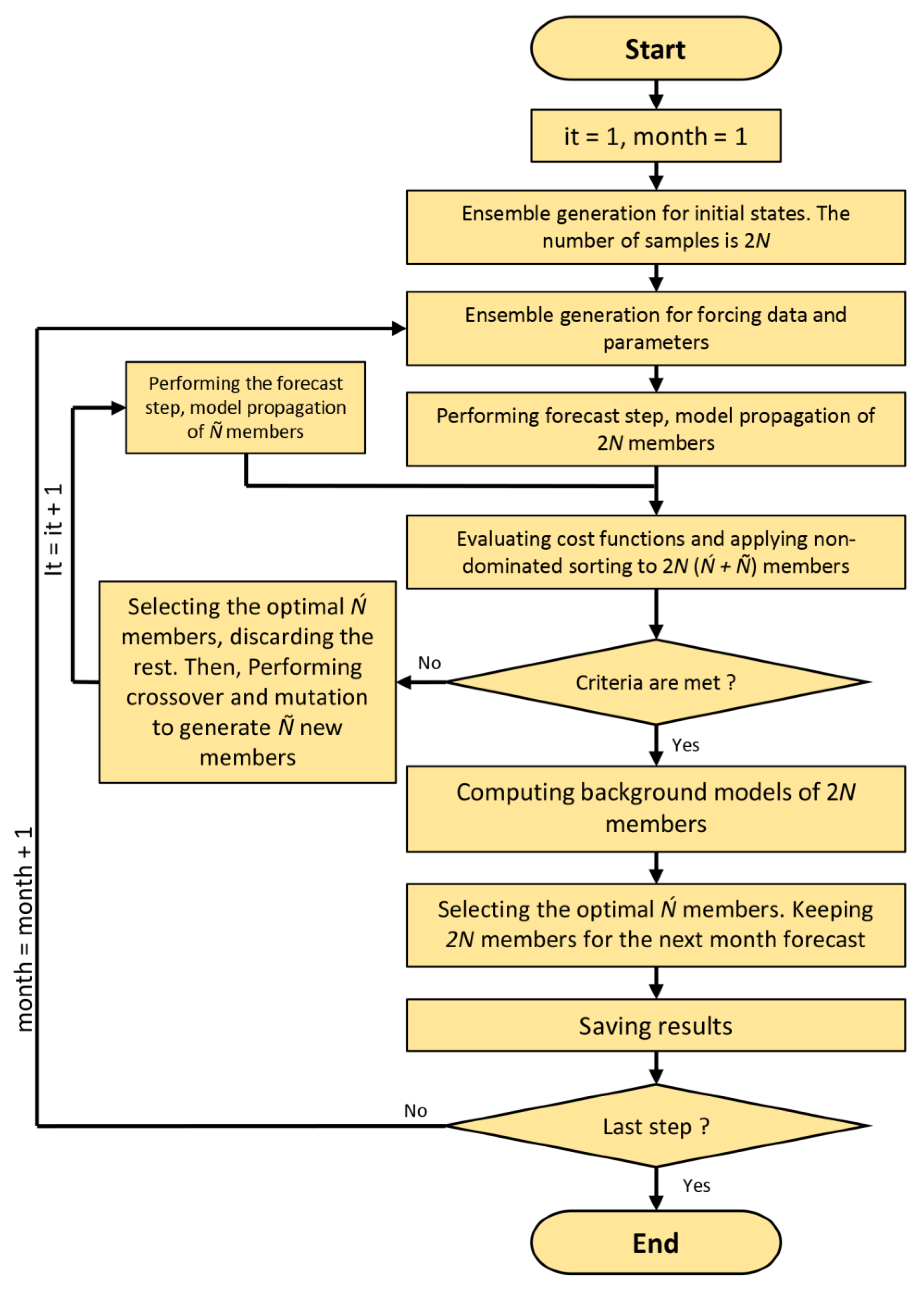
3.5. Evolutionary Smoother (EvS)

The EvS determines the optimal state estimates using an iterative process. Unlike other DA algorithms, EvS uses 2N = 200 ensemble members. In each iteration, EvS ranks the ensemble members based on a cost function ( J ):
  J i = j = 1 s { ( d j d b , j ) 2 σ b 2 + ( d j d y , j ) 2 σ y 2 } i
where d j is a model forecast of day j , d b is a value obtained from a background model, d y is a perturbed observation, σ b 2 is a variance of a background model, and σ y 2 is a variance of the observation (see Appendix D). Figure 3 illustrates EvS processes in detail. In a nutshell, EvS selects the N best samples in each iteration. These selected samples are used to generate N = 100 new offspring using crossover and mutation operations [17]. The crossover operator produces new members from the existing population, whereas mutation generates members outside the ensemble distribution. The mutation operator has the advantage of increasing the sample diversity of the DA system, which can alleviate ensemble collapse problems. The iteration process is repeated with 2N samples until the desired criteria are met—the cost functions are smaller than the observation uncertainty, i.e., 0.04 m3/m3 (soil moisture) and 2 cm (TWS), or the iteration number is greater than 50.

4. Results

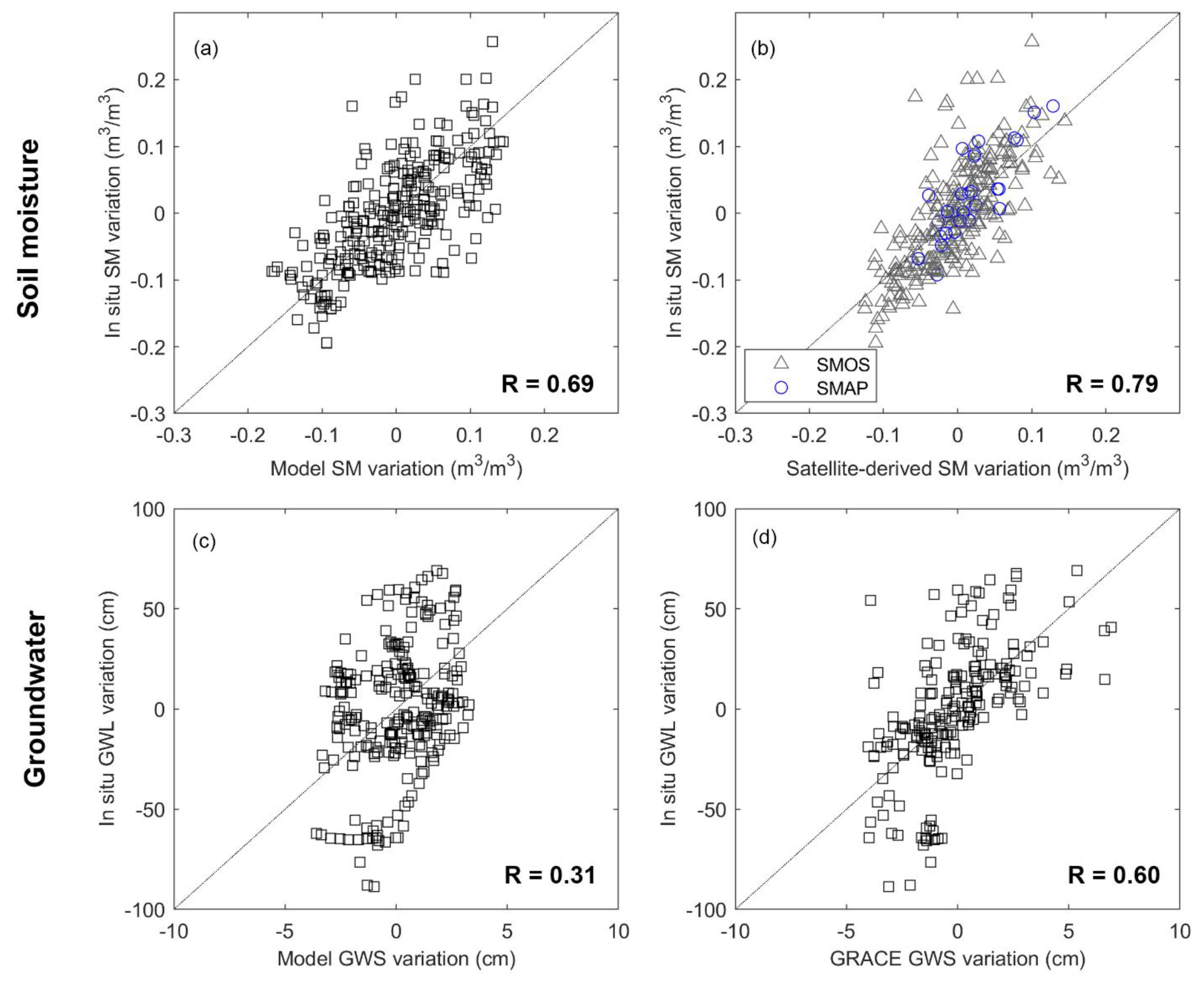
4.1. Initial Comparison

The benefit of assimilating satellite data can be preliminarily evaluated by comparing model estimates and satellite observations with in situ data. Open-loop (OL) SM and GWS variations are used here, meaning that the model simulation is performed without the use of DA. The SM and GWS variations are calculated by removing the long-term mean SM (or GWS) from their daily estimates. The SM evaluation (Figure 4a,b) reveals that SMOS/SMAP data have better agreement with the ground observations than the model, with a 0.1 higher correlation coefficient (see values given in Figure 4). Similar behavior is seen in GWS estimates, where GRACE-derived GWS (Figure 4d) provides a nearly 100% higher correlation value than the model (i.e., from 0.3 to 0.6). Note that the GRACE-derived GWS used in this comparison is simply calculated by subtracting the CABLE-simulated SM storage value from the GRACE observations. This preliminary analysis suggests that assimilating SMOS, SMAP, and GRACE data into CABLE may improve SM and GWS estimates in the Goulburn catchment (i.e., move model estimates closer to the values of ground observations). We performed an accuracy assessment in Section 4.4 to confirm this hypothesis.

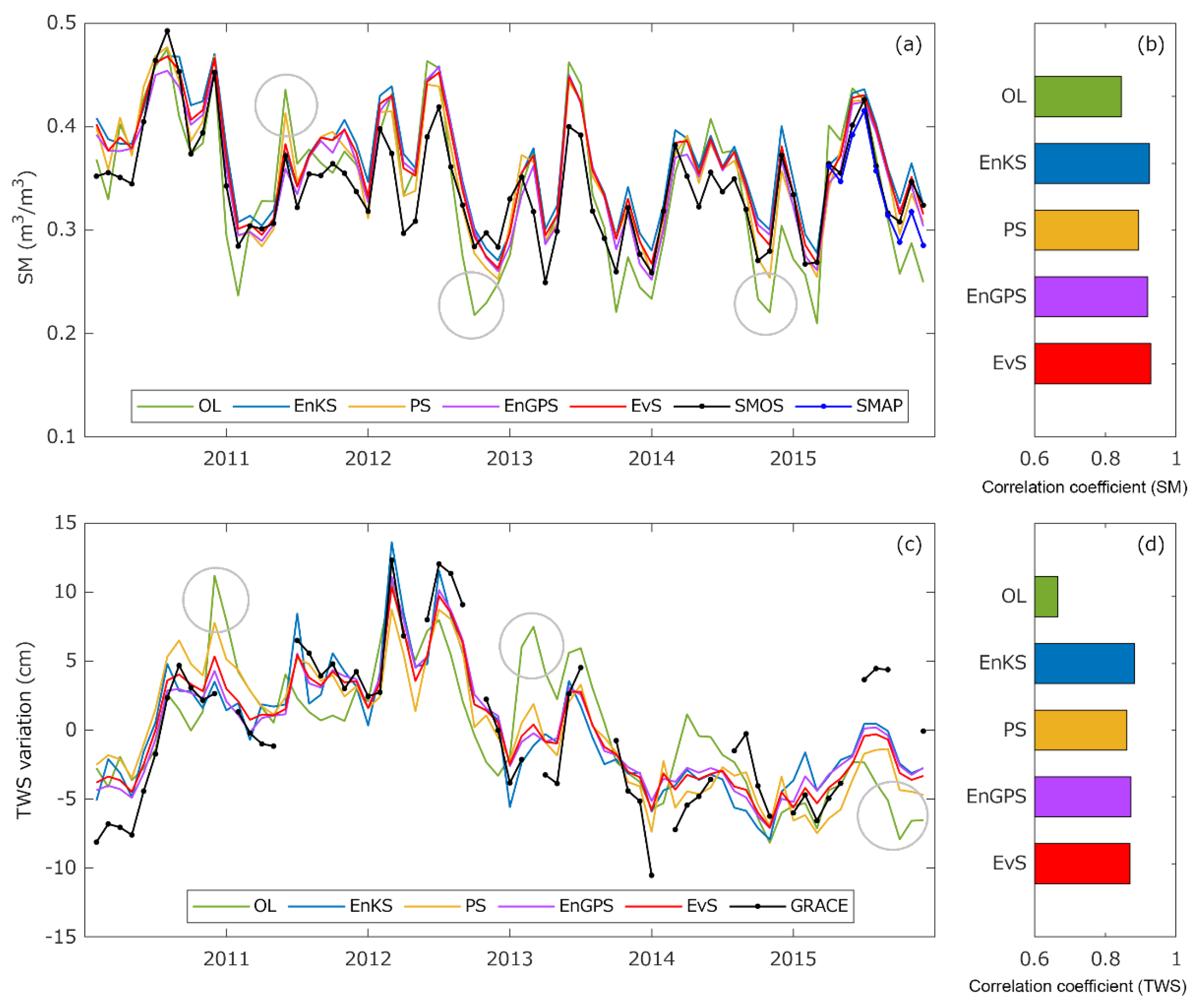
4.2. Multivariate DA Impacts on SM and TWS Estimates

The behavior of different multivariate DA algorithms is investigated by assessing their impact on SM and TWS estimates. The purpose of this analysis is to examine how DA affects model state estimates, while validation against ground measurements is discussed later in Section 4.4. The basin-averaged SM (Figure 5a) and TWS variations (Figure 5c) show that model simulations (OL) perform reasonably well compared to satellite observations, with correlation values greater than 0.6 (Figure 5b,d). However, under/overestimated SM and TWS are frequently observed in OL simulations, where model outputs differ significantly from observations: see, for example, SM estimates in 2011, 2012, and 2014 (gray circles in Figure 5a). Applying multivariate DA results in the SM and TWS estimates moving toward the assimilated observations and mitigates most of the significant mismatches between modeled and observed values (see, e.g., OL vs. EvS time series in Figure 5a,c). The correlation coefficients of SM and TWS estimates are improved by more than 0.1 through the inclusion of multivariate DA.
All four DA algorithms deliver relatively similar SM and TWS estimates. Among all considered DA approaches, EvS has the greatest impact on SM estimates and produces the highest correlation coefficient (Figure 5b). EvS also improves TWS estimates, with a correlation value only ~0.01 less than EnKS and EnGPS results (Figure 5d), suggesting that EvS is effective at capturing the assimilated observations. For both SM and TWS, EnGPS correlation coefficients fall between those of EnKS and PS. This is because EnGPS evaluates optimal particles using information from both EnKS (e.g., proposal function) and PS (e.g., likelihood function), resulting in posterior estimates that are constrained by the EnKS and PS results.

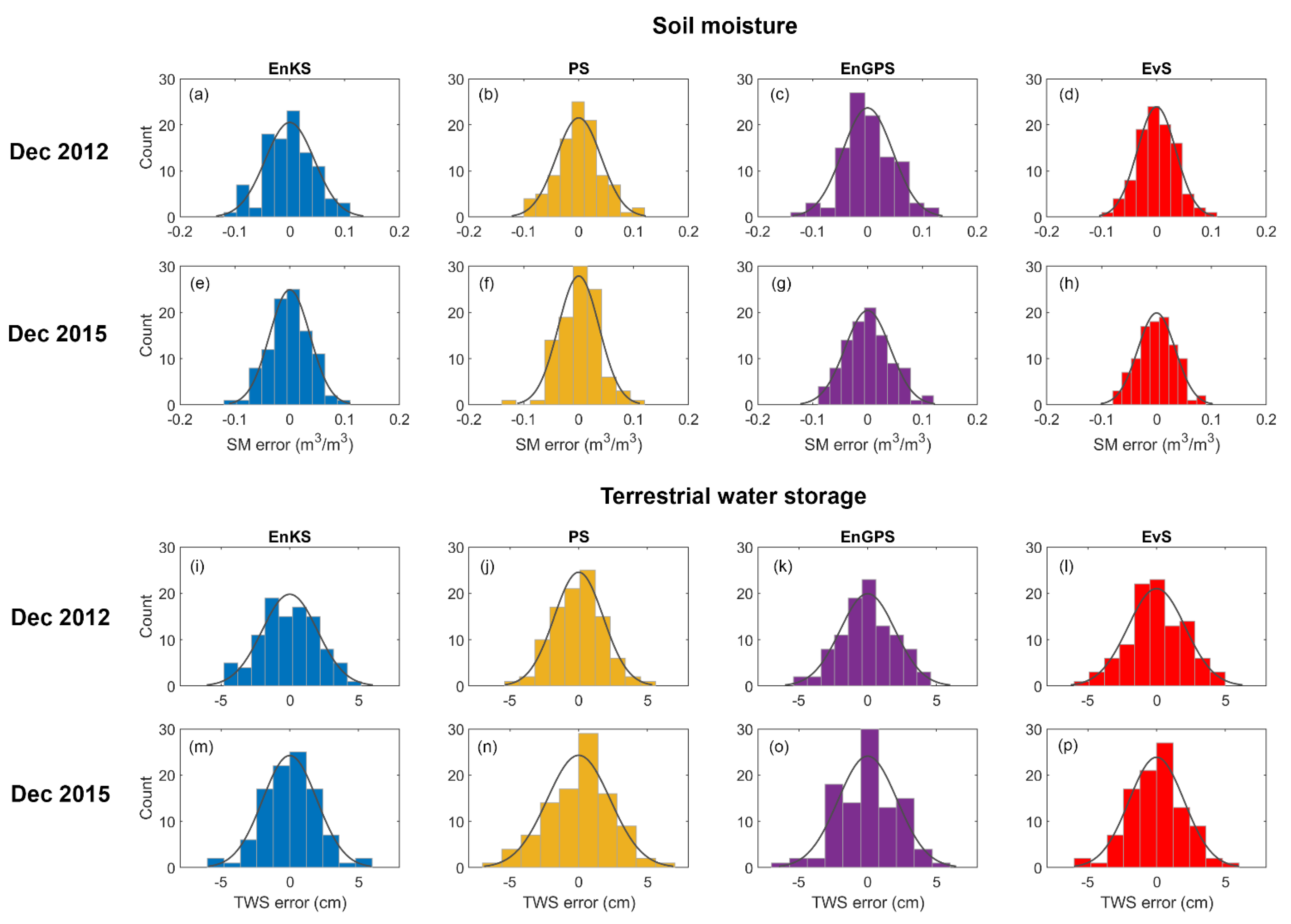
4.3. Error Characteristics of DA Systems

The four multivariate DA algorithms each have a unique approach to handling system errors. EnKS assumes Gaussian error distributions, while EvS, PS, and EnGPS are free from such a restriction. The success of EnKS (Figure 5) suggests that the error distribution of DA systems is probably Gaussian. To investigate this hypothesis, the error distribution of monthly basin-averaged SM and TWS estimates from four DA algorithms is determined at each analysis step. Error distributions from Dec 2012 and Dec 2015 are shown in Figure 6. Other monthly solutions exhibit a similar pattern. The Jarque–Bera (JB [39]) test is performed to confirm the validity of the Gaussian error assumption. Although some skewness of the error distribution is observed, we find that the SM and TWS error distributions in this study are close to Gaussian throughout the simulation period (at 0.05 significance level). The imperfect Gaussian shape of the error distribution seen in some panels of Figure 6 is due to the small sample size used in our DA systems. Increasing the number of ensemble members improves the Gaussian shape but has no effect on DA performance (not shown).

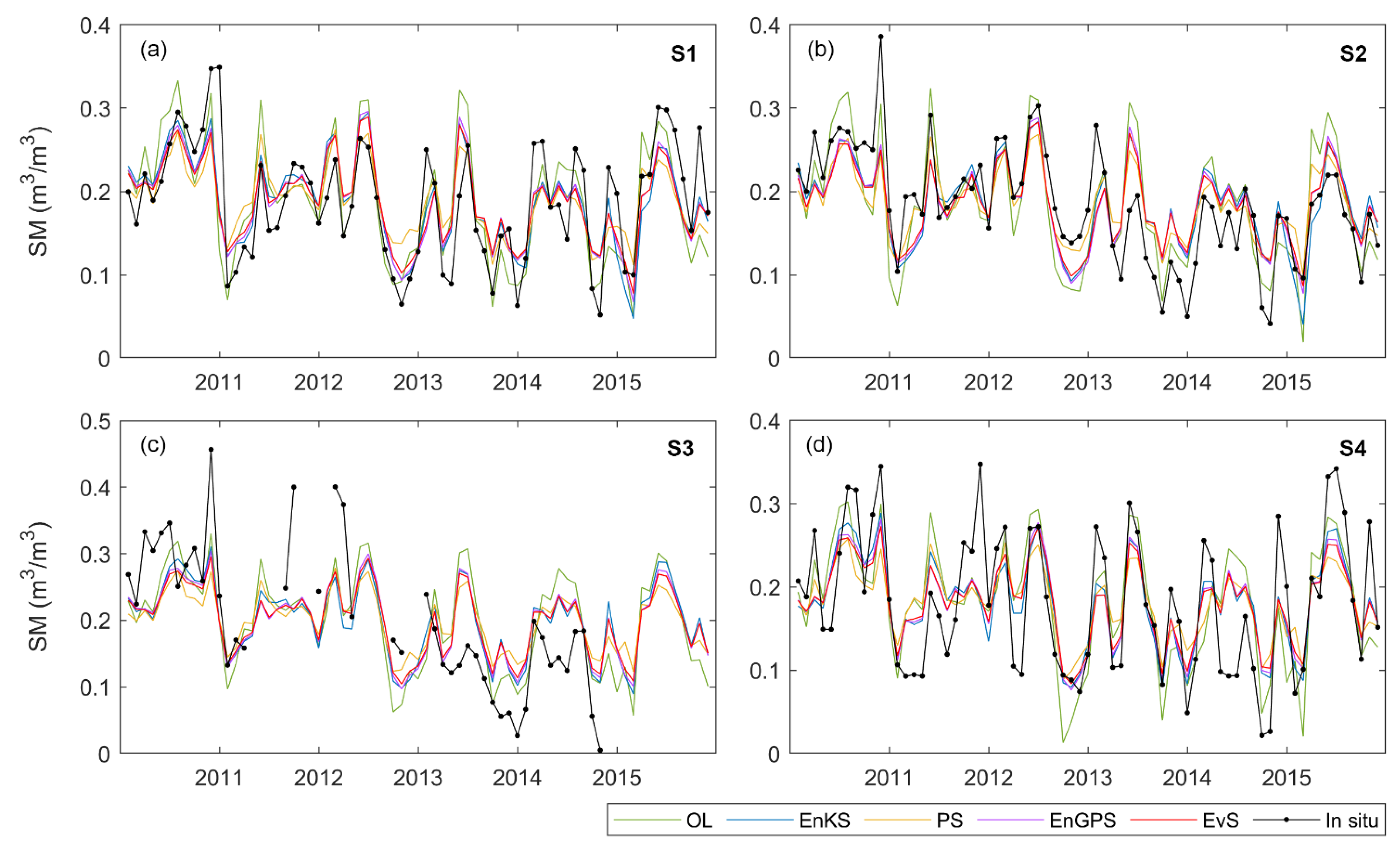
4.4. Validation with In Situ Data

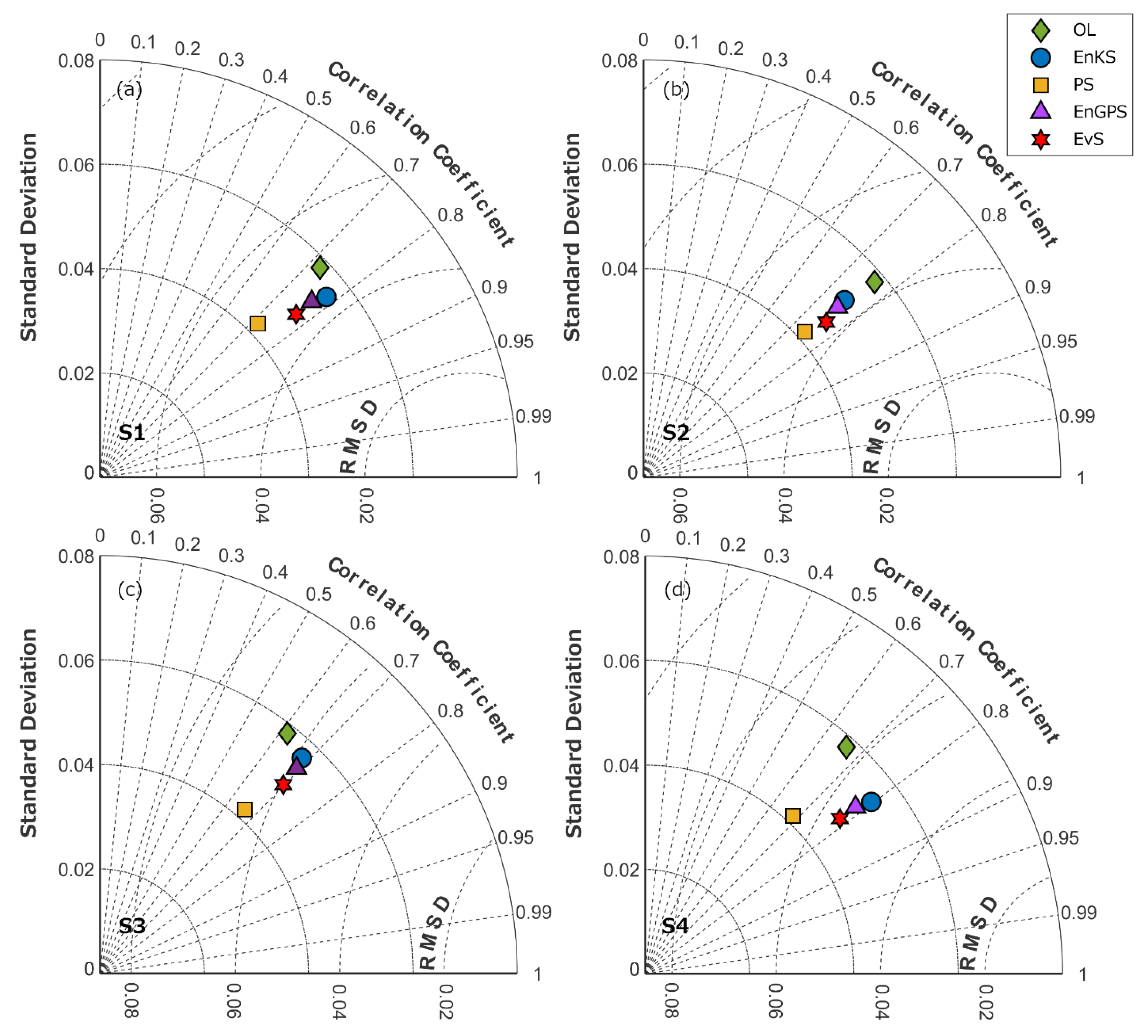
4.4.1. Soil Moisture

SM estimates are validated with in situ data at S1–S4 grid cells (see Figure 1). The four DA SM estimates exhibit similar temporal patterns but are noticeably distinct from the OL estimates (Figure 7). Utilizing multivariate DA leads to improved agreement between SM estimates and in situ data. Both OL and DA appear to be smoother than the ground truths, which is most likely due to a coarse spatial resolution of the model that is incapable of capturing point-scale SM variations. Despite this potential over-smoothing, OL and DA effectively observe the SM’s overall pattern. The declining tendency in SM between 2010 and 2015 is seen at all sites and results from reductions in precipitation since 2010 (Figure 8).
Figure 9 depicts the statistical results of SM estimates. Multivariate DA algorithms improve SM accuracy by increasing the correlation coefficient and reducing unbiased root mean square difference (RMSD [40]) by up to 20% (see, e.g., Figure 9d). EvS provides the best overall performance, improving correlation and RMSD values by up to 0.14 and 0.01 m3/m3, respectively. EnKS and EnGPS perform similarly to EvS, while PS performs slightly worse. It should be noted that the PS generates particles solely based on the model’s prior distribution, which does not always overlap with observation distributions [15]. This process can cause SM estimates to be closer to modeled than observed values at some update time steps. Multivariate DA provides correlation coefficients as high as 0.8. These results are in line with our initial analysis (Section 4.1), in which comparisons of satellite SM observations and in situ data yield similar correlation values (see, e.g., Figure 4b). This behavior is expected since the top soil component is directly updated by SMOS/SMAP data, i.e., via cost function (EvS), Kalman gain (EnKS), or likelihood (PS, EnGPS). The positive impact of satellite SM observations is simply propagated into modeled SM estimates. At S2, the positive impact of DA is marginal. The OL SM simulation at S2 has the highest correlation and lowest RMSD among the evaluated locations, and the slight impact of DA is due to the OL estimate already having very high accuracy in the first place.

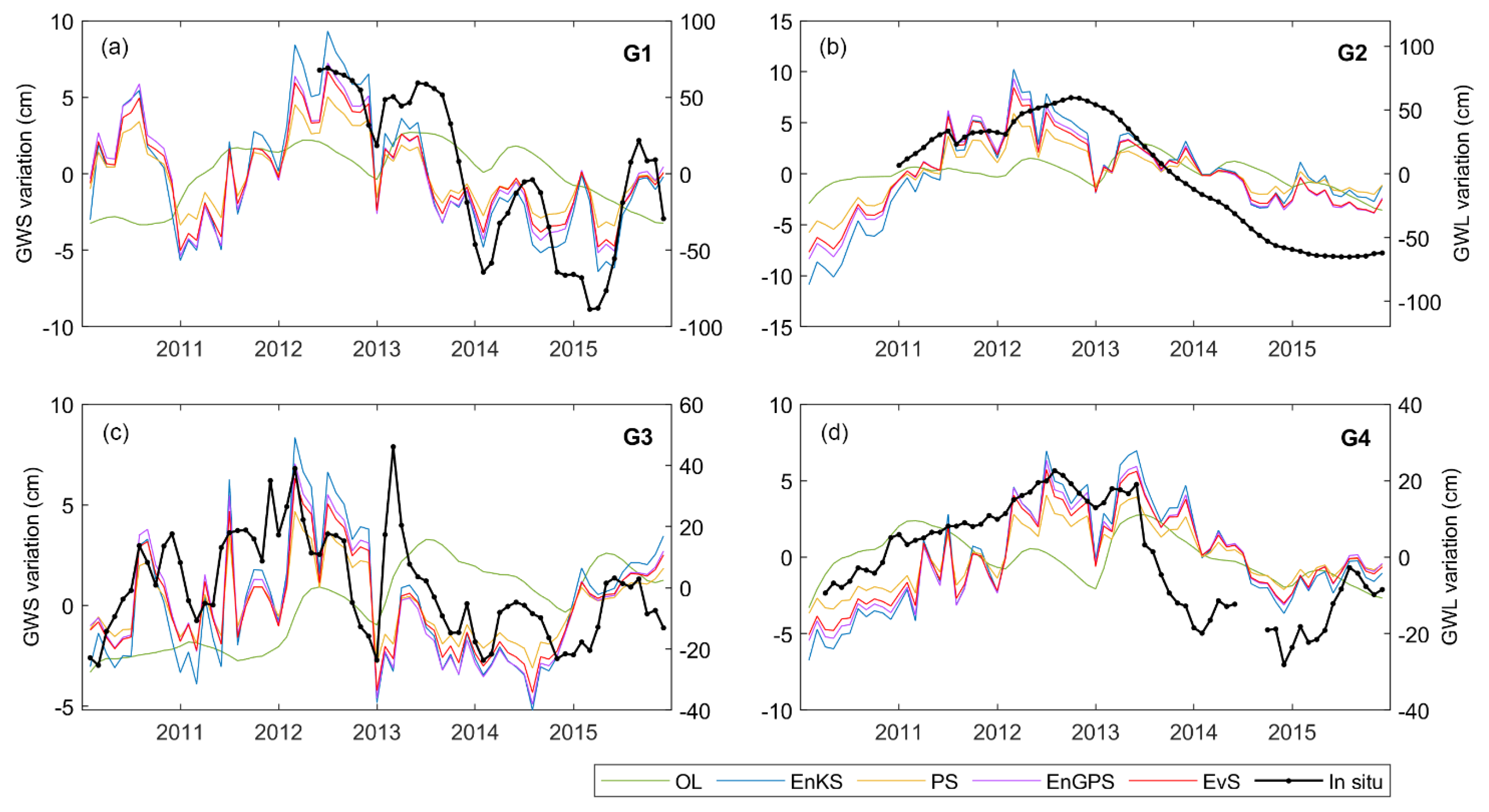
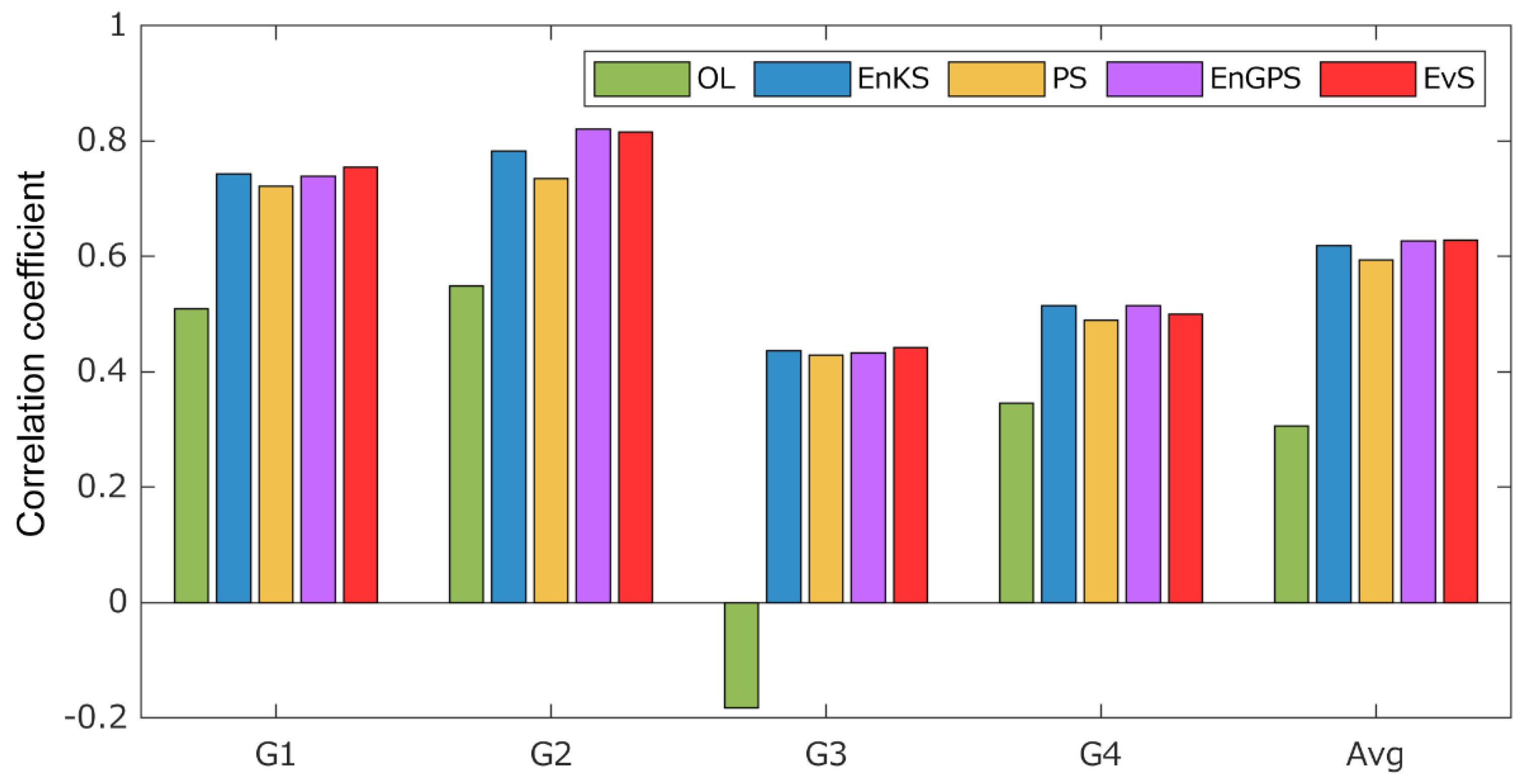
4.4.2. Groundwater Storage

GWS estimates are compared with in situ GWL at G1–G4 grid cells (Figure 10). Due to the lack of accurate specific yield, the conversion between GWS and groundwater level was not performed here, and the validation was only carried out in terms of correlation. OL GWS estimates have much smaller dynamic ranges than those of in situ data (e.g., Figure 10a). Ineffective redistribution between evapotranspiration and soil infiltration by CABLE (as described in Decker et al. [41]) likely causes inaccurate groundwater recharge and GWS variations. In addition, long-term trends in OL GWS estimates contradict ground truths, such as at G3, where OL exhibits increasing GWS (1 cm/yr), but in situ data shows decreasing GWL (−3 cm/yr). After applying multivariate DA, the overall GWS temporal feature is consistent with in situ data: GWS increases from 2010 to 2012 and decreases from 2013 to 2014, consistent with precipitation patterns (Figure 8). Multivariate DA also increases the GWS dynamic range and the seasonal variation in the GWS time series from 1.7 cm (OL) to 3 cm (DA) (see, e.g., Figure 10a). The performance of all four DA approaches is comparable.
The correlation coefficient between GWS and in situ GWL confirms the importance of multivariate DA in GWS estimations (Figure 11). To start, OL has a poor agreement with in situ GWL, with an average correlation value of only ~0.3 (see Avg in Figure 11). At G3, OL even exhibits anticorrelation. On average, applying multivariate DA increases correlation coefficients by about a factor of two (100%). EvS has the highest average correlation coefficient, 0.63. However, the advantage of EvS over the other three DA algorithms is marginal and statistically insignificant, according to the Fisher Z-transform test for correlation coefficients at a significance level of 0.05 [42]. This is due to the fact that EnKS, PS, and EnGPS all perform well under SM/TWS Gaussian error distributions (as demonstrated in Section 4.3). This analysis finds that all DA algorithms are suitable for GWS estimations in the Goulburn River catchment.

5. Discussion

Assimilating SMOS, SMAP, and GRACE data into CABLE in the Goulburn River catchment results in improved SM and GWS estimates. Our findings support those of previous studies [6,9,10] regarding the benefits of multivariate DA in simultaneously improving modeled SM and GWS. The assimilation of SMOS and SMAP leads to a 20% improvement in SM correlation and RMSD. GRACE DA results in a twofold (100%) increase in agreement between GWS estimates and in situ groundwater data. Despite marginal differences among DA approaches, the benefit of multivariate DA is in line with the findings shown in Tangdamrongsub et al. [10]. This indicates that the different update time window, whether monthly or sub-monthly, has no significant effect on DA performance in the Goulburn River catchment. However, the importance of time windows may differ depending on location, so a sensitivity analysis is always recommended prior to performing DA to determine the appropriate forecast/update period.
EvS has a significant impact on SM and GWS estimates, providing the most-improved correlation value among all DA approaches (EnKS, PS, and EnGPS). However, the degree of improvement of EvS does not differ significantly from the others. The similarity in DA performances is due to the system’s error distributions being close to Gaussian, which conforms with EnKS, PS, and EnGPS requirements. The small benefit of EvS over the other DA algorithms is a result of the latter having effective performance to begin with. In systems with highly non-Gaussian error distributions, EvS is expected to provide a more significant advantage [15,20].
From an implementation point of view, EvS is more robust than other algorithms because the relationship between model states and observations does not need to be formulated in a single large covariance matrix, as in, e.g., EnKS and EnGPS (see Equations (A1)–(A3)). This advantage is especially noticeable when a large number of model state variables or satellite observations are included in multivariate DA. In a large dimensional system, EvS requires less processor memory than other DA algorithms (i.e., EnKS, PS, and EnGPS). The crossover and mutation resampling in EvS also acts to improve the sample diversity of the DA system, avoiding the ensemble/particle collapse problems of PS [16]. The only disadvantage of EvS is that the iteration process can occasionally consume more simulation time than other DA algorithms, particularly in large study areas. However, the additional processing effort is found to be insignificant and does not affect EvS’s overall performance in our analysis.
Future developments may include different satellite SM and TWS observations, such as SM retrieval from the Cyclone Global Navigation Satellite System (CYGNSS [43]), and TWS derived from the Swarm satellites [44]. Including different observed variables such as leaf area index or snowcover in a multivariable DA algorithm is also feasible with minor changes to the state vector and measurement operator matrix. However, it should be noted that assimilating a large number of observations does not always result in improved simulation results, and a sensitivity study is recommended prior to the DA operation to identify the optimal set of assimilated observations.

6. Conclusions

This study assessed the performance of four different multivariate DA algorithms used to assimilate SMOS, SMAP, and GRACE data into the CABLE model to improve SM and GWS simulations in the Goulburn River catchment in Australia. The evaluation found that EvS improves the accuracy of SM and GWS estimates most, increasing their correlation with in situ observations by ~20% and 100%, respectively. Similar improvements were made by the other three DA approaches evaluated (EnKS, PS, and EnGPS). The similarity among DA performances can be explained by TWS error distributions being close to Gaussian. EvS may be superior in applications that contain highly non-Gaussian distributions (e.g., streamflow estimations; Dumedah and Coulibaly, 2013). In the context of water storage estimates, EvS demonstrates its utility in multivariate DA by simultaneously improving a suite of model state variables, resulting in a more robust DA system.

Author Contributions

Conceptualization, N.T.; methodology, N.T. and J.D.; validation and formal analysis, N.T.; writing—review and editing, N.T., J.D. and P.S. All authors have read and agreed to the published version of the manuscript.

Funding

This study received no external funding.

Informed Consent Statement

Not applicable.

Data Availability Statement

Data used in this paper are publicly available. Data access is described in Section 2.

Acknowledgments

N.T. was supported by the NASA Earth Science Division in support of the National Climate Assessment. We thank four anonymous reviewers who provided feedback on the paper.

Conflicts of Interest

The authors declare no conflict of interest.

Appendix A. Ensemble Kalman Smoother (EnKS)

In EnKS, the state vector is updated as follows:
x s | s i = x s | t 1 i + K ( y s i H x s | t 1 i ) ,
with
K = P e H T ( H P e H T + R e ) 1 ,
where y s i is a perturbed observation vector, K is the Kalman gain matrix, and P e and R e are the ensemble error covariance matrices of the model and observations, respectively. If the matrix A contains the ensemble states (SM and GWS) and A ¯ has the same dimension as A and filled in with the mean value computed from all ensemble members, P e can be computed as follows:
P e = ( A A ¯ ) ( A A ¯ ) T / ( N 1 ) .
Similarly, R e is computed as follows:
R e = Υ Υ T / ( N 1 ) ,
where Υ contains measurement errors of all ensemble members.

Appendix B. Particle Smoother (PS)

The PS represents the state probability density function (pdf) from random samples (called particles). The posterior pdf can be approximated using a set of weighted particles as follows:
p ( x s | y 1 : t ) = i = 1 N w ˜ s i δ ( x s x s i ) ,
where w ˜ i is a normalized importance weight associated with a particle x i , and δ (   ) is the Dirac delta function. The importance weight can be computed using a likelihood function p ( y s | x s i ) as:
w s i = w t 1 i · p ( y s | x s i ) .  
The likelihood function is expressed as
p ( y s | x s i ) = 1 ( 2 π ) N 0 2 det ( R ) 1 2 e [ 1 2 ( y s H x s i ) T R 1 ( y s H x s i ) ] ,
where det (   ) is a determinant of the given matrix, N 0 is a number of observations, and R is an observation error covariance matrix. The normalized importance weight is then computed as
w ˜ s i = w s i i = 1 N w s i .
Final outputs of PS approach consist of a particle set (in x s i ) and their associated weights ( w ˜ s i ). The weighted mean of the particles represents the optimal state estimate.

Appendix C. Ensemble Gaussian Particle Smoother (EnGPS)

The EnGPS is developed based on Ensemble Gaussian Particle Filter [45]. The EnGPS adopts the same concept as PS, but computes importance weights based on the posterior estimate of EnKS:
w s i = p ( y s | x s | s i ) p ( x s i | y t 1 ) q ( x s | s i , y s )
where p ( y s | x s | s i ) ,   p ( x s i | y t 1 ) , and q ( x s | s i , y s ) are a likelihood, prior, and proposal density function, respectively. The x s | s i represents particles obtained from a proposal density function q ( x s | s i , y s ) . constructed based on EnKS posterior information. The likelihood function can be calculated using Equation (A7) by replacing x s i . with x s | s i . The prior and proposal functions are approximated using a Gaussian distribution as follows:
p ( x s i | y t 1 ) = N ( x s | s i ; x ¯ s | t 1 , P s | t 1 ) ,  
q ( x s | s i , y s ) = N ( x s | s i ; x ¯ s | s , P s | s ) ,  
x ¯ s | t 1 = 1 N i = 1 N x s | t 1 i ,  
x ¯ s | s = 1 N i = 1 N x s | s i ,  
P s | t 1 = 1 N 1 i = 1 N ( x s | t 1 i x ¯ s | t 1 ) ( x s | t 1 i x ¯ s | t 1 ) T ,
P s | s = 1 N 1 i = 1 N ( x s | s i x ¯ s | s ) ( x s | s i x ¯ s | s ) T ,  
where x s | t 1 i and x s | s i represent particles obtained after the model propagation and approximated from EnKS estimates, respectively. After obtaining w s i , the normalized weight is computed as w ˜ s i = w s i / i = 1 N w s i . Then, the posterior pdf can be finally defined as:
p ( x s | y 1 : t ) = N ( x s ; x ^ s | s , P ^ s | s ) ,  
where x ^ s | s and P ^ s | s are the weighted mean and weighted covariance, which are computed as follows:
x ^ s | s = i = 1 N w ˜ s i   x s | s i ,  
P ^ s | s = i = 1 N w ˜ s i   ( x s | s i x ^ s | s ) ( x s | s i x ^ s | s ) T  

Appendix D. Evolutionary Smoother (EvS)

The EvS approach employs a genetic algorithm to determine the optimal solution through a natural selection process. In the analysis step, the cost function ( J ) is computed as follows:
J i = j = 1 s { ( d j d b , j ) 2 σ b 2 + ( d j d y , j ) 2 σ y 2 } i
where d j is a model forecast of day j , d b is a value obtained from a background model, d y is a perturbed observation, σ b 2 is a variance of a background model, and σ y 2 is a variance of the observation. In line with Dumedah [17], a background model ( d b , σ b 2 ) is obtained from the mean and variance of ensemble members in previous time steps. For the first time step, a randomly generated value is used as the background model.
After obtaining the cost function with respect to SMOS, SMAP, and GRACE observations, EvS uses the Non-dominated Sorting Genetic Algorithm-II (NSGA-II [46]) algorithm to evaluate the goodness-of-fit for each forecast ensemble member. This sorting process identifies the optimal Ń = 100 members that have the best agreements with observations. These selected Ń ensemble members are kept for the next iteration, while the others (remaining members) are discarded.
Crossover and mutation are used to generate Ñ = 100 new offspring. The crossover operator produces new ensemble members from within the existing population, whereas mutation can generate members from outside the ensemble distribution. An advantage of the mutation operator is an increased sample diversity of the DA system, which can ease ensemble collapse problems. The newly generated Ñ members are used in the forecast and analysis steps (Equations (1)–(6)) to obtain the cost functions associated with them. Then, the sorting process is repeated on the basis of Ń (optimal) + Ñ (newly generated) = 2N members to determine the new optimal Ń members. This iterative process continues until the cost functions are smaller than the observation uncertainty, i.e., 0.04 m3/m3 (soil moisture) and 2 cm (TWS), or the iteration number is greater than 50. After the iteration is completed, the last day’s model states are used as initial states for the following month’s forecast. The updated model states are used as the background model ( d b , σ b 2 ).

References

  1. Pitman, A.J. The Evolution of, and Revolution in, Land Surface Schemes Designed for Climate Models. Int. J. Climatol. 2003, 23, 479–510. [Google Scholar] [CrossRef]
  2. Moradkhani, H. Hydrologic Remote Sensing and Land Surface Data Assimilation. Sensors 2008, 8, 2986–3004. [Google Scholar] [CrossRef] [PubMed]
  3. Reichle, R.H. Data Assimilation Methods in the Earth Sciences. Adv. Water Resour. 2008, 31, 1411–1418. [Google Scholar] [CrossRef]
  4. Yin, W.; Han, S.-C.; Zheng, W.; Yeo, I.-Y.; Hu, L.; Tangdamrongsub, N.; Ghobadi-Far, K. Improved Water Storage Estimates within the North China Plain by Assimilating GRACE Data into the CABLE Model. J. Hydrol. 2020, 590, 125348. [Google Scholar] [CrossRef]
  5. Yan, H.; Moradkhani, H. Combined Assimilation of Streamflow and Satellite Soil Moisture with the Particle Filter and Geostatistical Modeling. Adv. Water Resour. 2016, 94, 364–378. [Google Scholar] [CrossRef] [Green Version]
  6. Tian, S.; Tregoning, P.; Renzullo, L.J.; van Dijk, A.I.J.M.; Walker, J.P.; Pauwels, V.R.N.; Allgeyer, S. Improved Water Balance Component Estimates through Joint Assimilation of GRACE Water Storage and SMOS Soil Moisture Retrievals. Water Resour. Res. 2017, 53, 1820–1840. [Google Scholar] [CrossRef]
  7. Sabater, J.M.; Rüdiger, C.; Calvet, J.-C.; Fritz, N.; Jarlan, L.; Kerr, Y. Joint Assimilation of Surface Soil Moisture and LAI Observations into a Land Surface Model. Agric. For. Meteorol. 2008, 148, 1362–1373. [Google Scholar] [CrossRef] [Green Version]
  8. Montzka, C.; Pauwels, V.R.N.; Franssen, H.-J.H.; Han, X.; Vereecken, H. Multivariate and Multiscale Data Assimilation in Terrestrial Systems: A Review. Sensors 2012, 12, 16291–16333. [Google Scholar] [CrossRef] [Green Version]
  9. Girotto, M.; Reichle, R.H.; Rodell, M.; Liu, Q.; Mahanama, S.; De Lannoy, G.J.M. Multi-Sensor Assimilation of SMOS Brightness Temperature and GRACE Terrestrial Water Storage Observations for Soil Moisture and Shallow Groundwater Estimation. Remote Sens. Environ. 2019, 227, 12–27. [Google Scholar] [CrossRef]
  10. Tangdamrongsub, N.; Han, S.-C.; Yeo, I.-Y.; Dong, J.; Steele-Dunne, S.C.; Willgoose, G.; Walker, J.P. Multivariate Data Assimilation of GRACE, SMOS, SMAP Measurements for Improved Regional Soil Moisture and Groundwater Storage Estimates. Adv. Water Resour. 2020, 135, 103477. [Google Scholar] [CrossRef]
  11. Reichle, R.H.; McLaughlin, D.B.; Entekhabi, D. Hydrologic Data Assimilation with the Ensemble Kalman Filter. Mon. Weather Rev. 2002, 130, 103–114. [Google Scholar] [CrossRef] [Green Version]
  12. Evensen, G. The Ensemble Kalman Filter: Theoretical Formulation and Practical Implementation. Ocean Dyn. 2003, 53, 343–367. [Google Scholar] [CrossRef]
  13. Ott, E.; Hunt, B.R.; Szunyogh, I.; Zimin, A.V.; Kostelich, E.J.; Corazza, M.; Kalnay, E.; Patil, D.J.; Yorke, J.A. A Local Ensemble Kalman Filter for Atmospheric Data Assimilation. Tellus Dyn. Meteorol. Oceanogr. 2004, 56, 415–428. [Google Scholar] [CrossRef]
  14. Krymskaya, M.V.; Hanea, R.G.; Verlaan, M. An Iterative Ensemble Kalman Filter for Reservoir Engineering Applications. Comput. Geosci. 2009, 13, 235–244. [Google Scholar] [CrossRef] [Green Version]
  15. Weerts, A.H.; El Serafy, G.Y.H. Particle Filtering and Ensemble Kalman Filtering for State Updating with Hydrological Conceptual Rainfall-Runoff Models. Water Resour. Res. 2006, 42, W09403. [Google Scholar] [CrossRef] [Green Version]
  16. Moradkhani, H.; Hsu, K.-L.; Gupta, H.; Sorooshian, S. Uncertainty Assessment of Hydrologic Model States and Parameters: Sequential Data Assimilation Using the Particle Filter. Water Resour. Res. 2005, 41, W05012. [Google Scholar] [CrossRef] [Green Version]
  17. Dumedah, G. Formulation of the Evolutionary-Based Data Assimilation, and Its Implementation in Hydrological Forecasting. Water Resour. Manag. 2012, 26, 3853–3870. [Google Scholar] [CrossRef]
  18. Chemin, Y.; Honda, K. Spatiotemporal Fusion of Rice Actual Evapotranspiration With Genetic Algorithms and an Agrohydrological Model. IEEE Trans. Geosci. Remote Sens. 2006, 44, 3462–3469. [Google Scholar] [CrossRef]
  19. Ines, A.V.M.; Mohanty, B.P. Near-Surface Soil Moisture Assimilation for Quantifying Effective Soil Hydraulic Properties Using Genetic Algorithms: 2. Using Airborne Remote Sensing during SGP97 and SMEX02. Water Resour. Res. 2009, 45. [Google Scholar] [CrossRef] [Green Version]
  20. Dumedah, G.; Coulibaly, P. Evaluating Forecasting Performance for Data Assimilation Methods: The Ensemble Kalman Filter, the Particle Filter, and the Evolutionary-Based Assimilation. Adv. Water Resour. 2013, 60, 47–63. [Google Scholar] [CrossRef]
  21. Tangdamrongsub, N.; Han, S.-C.; Yeo, I.-Y. Enhancement of Water Storage Estimates Using GRACE Data Assimilation with Particle Filter Framework. In Proceedings of the 22nd International Congress on Modelling and Simulation (MODSIM), Hobart, TAS, Australia, 5 December 2017; pp. 1041–1047. [Google Scholar]
  22. Decker, M. Development and Evaluation of a New Soil Moisture and Runoff Parameterization for the CABLE LSM Including Subgrid-Scale Processes. J. Adv. Model. Earth Syst. 2015, 7, 1788–1809. [Google Scholar] [CrossRef]
  23. Kowalczyk, E.A.; Wang, Y.P.; Law, R.M.; Davies, H.L.; McGregor, J.L.; Abramowitz, G.S. The CSIRO Atmosphere Biosphere Land Exchange (CABLE) Model for Use in Climate Models and as an Offline Model; CSIRO Marine and Atmospheric Research: Aspendale, Australia, 2006; ISBN 978-1-921232-30-5. [Google Scholar]
  24. Rodell, M.; Houser, P.R.; Jambor, U.; Gottschalck, J.; Mitchell, K.; Meng, C.-J.; Arsenault, K.; Cosgrove, B.; Radakovich, J.; Bosilovich, M.; et al. The Global Land Data Assimilation System. Bull. Am. Meteorol. Soc. 2004, 85, 381–394. [Google Scholar] [CrossRef] [Green Version]
  25. Huffman, G.J.; Bolvin, D.T.; Braithwaite, D.; Hsu, K.; Joyce, R.; Kidd, C.; Nelkin, E.J.; Sorooshian, S.; Tan, J.; Xie, P. NASA Global Precipitation Measurement (GPM) Integrated Multi-SatellitE Retrievals for GPM (IMERG); Algorithm Theoretical Basis Document (ATBD)Version 06; NASAGSFC: Greenbelt, MD, USA, 2019.
  26. Tangdamrongsub, N.; Han, S.-C.; Decker, M.; Yeo, I.-Y.; Kim, H. On the Use of the GRACE Normal Equation of Inter-Satellite Tracking Data for Estimation of Soil Moisture and Groundwater in Australia. Hydrol. Earth Syst. Sci. 2018, 22, 1811–1829. [Google Scholar] [CrossRef] [Green Version]
  27. Rüdiger, C.; Hancock, G.; Hemakumara, H.M.; Jacobs, B.; Kalma, J.D.; Martinez, C.; Thyer, M.; Walker, J.P.; Wells, T.; Willgoose, G.R. Goulburn River Experimental Catchment Data Set. Water Resour. Res. 2007, 43, W10403. [Google Scholar] [CrossRef] [Green Version]
  28. Kerr, Y.H.; Waldteufel, P.; Richaume, P.; Wigneron, J.P.; Ferrazzoli, P.; Mahmoodi, A.; Bitar, A.A.; Cabot, F.; Gruhier, C.; Juglea, S.E.; et al. The SMOS Soil Moisture Retrieval Algorithm. IEEE Trans. Geosci. Remote Sens. 2012, 50, 1384–1403. [Google Scholar] [CrossRef]
  29. Entekhabi, D.; Njoku, E.G.; O’Neill, P.E.; Kellogg, K.H.; Crow, W.T.; Edelstein, W.N.; Entin, J.K.; Goodman, S.D.; Jackson, T.J.; Johnson, J.; et al. The Soil Moisture Active Passive (SMAP) Mission. Proc. IEEE 2010, 98, 704–716. [Google Scholar] [CrossRef]
  30. Bitar, A.A.; Mialon, A.; Kerr, Y.H.; Cabot, F.; Richaume, P.; Jacquette, E.; Quesney, A.; Mahmoodi, A.; Tarot, S.; Parrens, M.; et al. The Global SMOS Level 3 Daily Soil Moisture and Brightness Temperature Maps. Earth Syst. Sci. Data 2017, 9, 293–315. [Google Scholar] [CrossRef] [Green Version]
  31. Crow, W.T.; Koster, R.D.; Reichle, R.H.; Sharif, H.O. Relevance of Time-Varying and Time-Invariant Retrieval Error Sources on the Utility of Spaceborne Soil Moisture Products. Geophys. Res. Lett. 2005, 32, L24405. [Google Scholar] [CrossRef] [Green Version]
  32. Reichle, R.H.; Koster, R.D. Bias Reduction in Short Records of Satellite Soil Moisture. Geophys. Res. Lett. 2004, 31, L19501. [Google Scholar] [CrossRef] [Green Version]
  33. Lievens, H.; Tomer, S.K.; Al Bitar, A.; De Lannoy, G.J.M.; Drusch, M.; Dumedah, G.; Hendricks Franssen, H.-J.; Kerr, Y.H.; Martens, B.; Pan, M.; et al. SMOS Soil Moisture Assimilation for Improved Hydrologic Simulation in the Murray Darling Basin, Australia. Remote Sens. Environ. 2015, 168, 146–162. [Google Scholar] [CrossRef]
  34. Colliander, A.; Jackson, T.J.; Bindlish, R.; Chan, S.; Das, N.; Kim, S.B.; Cosh, M.H.; Dunbar, R.S.; Dang, L.; Pashaian, L.; et al. Validation of SMAP Surface Soil Moisture Products with Core Validation Sites. Remote Sens. Environ. 2017, 191, 215–231. [Google Scholar] [CrossRef]
  35. Save, H.; Bettadpur, S.; Tapley, B.D. High-Resolution CSR GRACE RL05 Mascons. J. Geophys. Res. Solid Earth 2016, 121, 7547–7569. [Google Scholar] [CrossRef]
  36. Tapley, B.D.; Bettadpur, S.; Ries, J.C.; Thompson, P.F.; Watkins, M.M. GRACE Measurements of Mass Variability in the Earth System. Science 2004, 305, 503–505. [Google Scholar] [CrossRef] [PubMed] [Green Version]
  37. Flechtner, F.; Neumayer, K.-H.; Dahle, C.; Dobslaw, H.; Fagiolini, E.; Raimondo, J.-C.; Güntner, A. What Can Be Expected from the GRACE-FO Laser Ranging Interferometer for Earth Science Applications? In Remote Sensing and Water Resources; Cazenave, A., Champollion, N., Benveniste, J., Chen, J., Eds.; Space Sciences Series of ISSI; Springer International Publishing: Cham, Switzerland, 2016; pp. 263–280. ISBN 978-3-319-32449-4. [Google Scholar]
  38. Wahr, J.; Swenson, S.; Velicogna, I. Accuracy of GRACE Mass Estimates. Geophys. Res. Lett. 2006, 33, L06401. [Google Scholar] [CrossRef] [Green Version]
  39. Jarque, C.M.; Bera, A.K. Efficient Tests for Normality, Homoscedasticity and Serial Independence of Regression Residuals. Econ. Lett. 1980, 6, 255–259. [Google Scholar] [CrossRef]
  40. Entekhabi, D.; Reichle, R.H.; Koster, R.D.; Crow, W.T. Performance Metrics for Soil Moisture Retrievals and Application Requirements. J. Hydrometeorol. 2010, 11, 832–840. [Google Scholar] [CrossRef]
  41. Decker, M.; Or, D.; Pitman, A.; Ukkola, A. New Turbulent Resistance Parameterization for Soil Evaporation Based on a Pore-Scale Model: Impact on Surface Fluxes in CABLE. J. Adv. Model. Earth Syst. 2017, 9, 220–238. [Google Scholar] [CrossRef] [Green Version]
  42. Steiger, J.H. Tests for Comparing Elements of a Correlation Matrix. Psychol. Bull. 1980, 87, 245–251. [Google Scholar] [CrossRef]
  43. Al-Khaldi, M.M.; Johnson, J.T. Soil Moisture Retrievals Using CYGNSS Data in a Time-Series Ratio Method: Progress Update and Error Analysis. IEEE Geosci. Remote Sens. Lett. 2022, 19, 1–5. [Google Scholar] [CrossRef]
  44. Teixeira da Encarnação, J.; Arnold, D.; Bezděk, A.; Dahle, C.; Doornbos, E.; van den IJssel, J.; Jäggi, A.; Mayer-Gürr, T.; Sebera, J.; Visser, P.; et al. Gravity Field Models Derived from Swarm GPS Data. Earth Planets Space 2016, 68, 127. [Google Scholar] [CrossRef] [Green Version]
  45. Plaza Guingla, D.A.; De Keyser, R.; De Lannoy, G.J.M.; Giustarini, L.; Matgen, P.; Pauwels, V.R.N. Improving Particle Filters in Rainfall-Runoff Models: Application of the Resample-Move Step and the Ensemble Gaussian Particle Filter. Water Resour. Res. 2013, 49, 4005–4021. [Google Scholar] [CrossRef]
  46. Deb, K.; Pratap, A.; Agarwal, S.; Meyarivan, T. A Fast and Elitist Multiobjective Genetic Algorithm: NSGA-II. IEEE Trans. Evol. Comput. 2002, 6, 182–197. [Google Scholar] [CrossRef] [Green Version]
Figure 1. The Goulburn River catchment in South−East Australia (see inset). The displayed gridlines denote the boundaries of model grid cells. The in situ SM and GWL data locations are represented by blue diamonds and red pentagons, respectively. All in situ SM data within the same model grid cell are averaged, resulting in S1–S4 grid cells. A similar approach is applied to the in situ GWL data, resulting in G1–G4 grid cells.
Water 14 00621 g001
Figure 2. The multivariate DA schematic used in this study. (a) In the forecast step, a model propagation of approximately one month is performed, and the daily model state variables (e.g., SM, GWS) are saved. (b) In the analysis step, satellite observations are used to update the state variables of the entire month. (c) The updated variables are saved, and the model states from the last day are used as initial states for the following month’s forecast.
Water 14 00621 g002
Figure 3. The processing diagram for EvS. The process employs genetic algorithms (e.g., crossover and mutation) to determine the best state estimates. N, Ń, and Ñ represent the number of ensembles. The different notations are used to clarify the processing step to which they belong; for example, Ń is the number of selecting ensembles, and Ñ is the number of newly generated ensemble members from crossover and mutation processes. The process is repeated until the cost functions are smaller than the observation uncertainties or the iteration number (it) exceeds 50.
Water 14 00621 g003
Figure 4. Initial comparisons between modeled/observed variables and in situ data, (a) modeled SM vs. in situ SM variations, (b) satellite−derived SM (SMOS/SMAP) vs. in situ SM variations, (c) modeled GWS vs. in situ GWL variations, and (d) satellite−derived GWS (GRACE GWS) vs. in situ GWL variations. For this initial analysis, GRACE GWS variations are computed by removing CABLE−simulated SM storage variations from GRACE observations. The correlation coefficient (R) is provided in each figure.
Water 14 00621 g004
Figure 5. (a,c) Monthly basin−averaged SM and TWS variations from OL and four different DA algorithms (EnKS, PS, EnGPS, and EvS). For comparison, SMOS/SMAP in (a) and GRACE observations in (c) are also shown. The circles represent the periods when model estimates differ significantly from observations. (b,d) Spearman’s correlation coefficients of SM (c) and TWS (d) computed between model estimates and satellite observations.
Water 14 00621 g005
Figure 6. Prior error distributions of the model−estimated SM (first (ad) and second rows (eh)) and TWS (third (il) and fourth rows (mp)) obtained from four DA algorithms in Dec 2012 and Dec 2015: EnKS (first column), PS (second column), EnGPS (third column), and EvS (fourth column). Gaussian fits to error distributions are shown in each figure as a solid black line.
Water 14 00621 g006
Figure 7. SM estimates from four DA approaches (EnKS, PS, EnGPS, and EvS) at S1–S4 pixels (ad). For comparison, OL estimates and in situ SM data are also shown.
Water 14 00621 g007
Figure 8. Monthly and annual basin-averaged precipitation (prec) obtained from the GLDAS data.
Water 14 00621 g008
Figure 9. Taylor diagrams of SM estimates from OL and four DA approaches (EnKS, PS, EnGPS, and EvS) at S1–S4 pixels (ad). Note that the horizontal scale (RMSD) varies depending on the location.
Water 14 00621 g009
Figure 10. GWS variations obtained from four DA approaches (EnKS, PS, EnGPS, and EvS) at G1–G4 pixels (ad). For comparison, OL estimates and in situ GWL variations are also shown.
Water 14 00621 g010
Figure 11. Correlation coefficients of GWS estimates obtained from OL and four DA approaches (EnKS, PS, EnGPS, and EvS) at G1−G4 pixels. Average correlation values (Avg) from all four locations are also shown.
Water 14 00621 g011
Table 1. Characteristics of the four DA algorithms evaluated in this study.
EnKSPSEnGPSEvS
Sample sizeNNN2N
Error distributionGaussianNo restrictionNo restrictionNo restriction
Evaluation approachKalman gain functionLikelihood functionLikelihood function and proposal distributionCost functions
Updating approachApplying Kalman gain functionResampling particles based on the likelihood functionResampling particles based on EnKS posterior estimatesNatural selection (crossover, mutation) through the iteration process
Posterior estimationMean of ensemble membersThe weighted mean of ensemble membersThe weighted mean of ensemble membersMean of ensemble members or only selecting optimal members
Publisher’s Note: MDPI stays neutral with regard to jurisdictional claims in published maps and institutional affiliations.

