

Physics-Informed Neural Networks-Based Salinity Modeling in the Sacramento–San Joaquin Delta of California
 , , ,
, , ,
Abstract
:1. Introduction
2. Materials and Methods
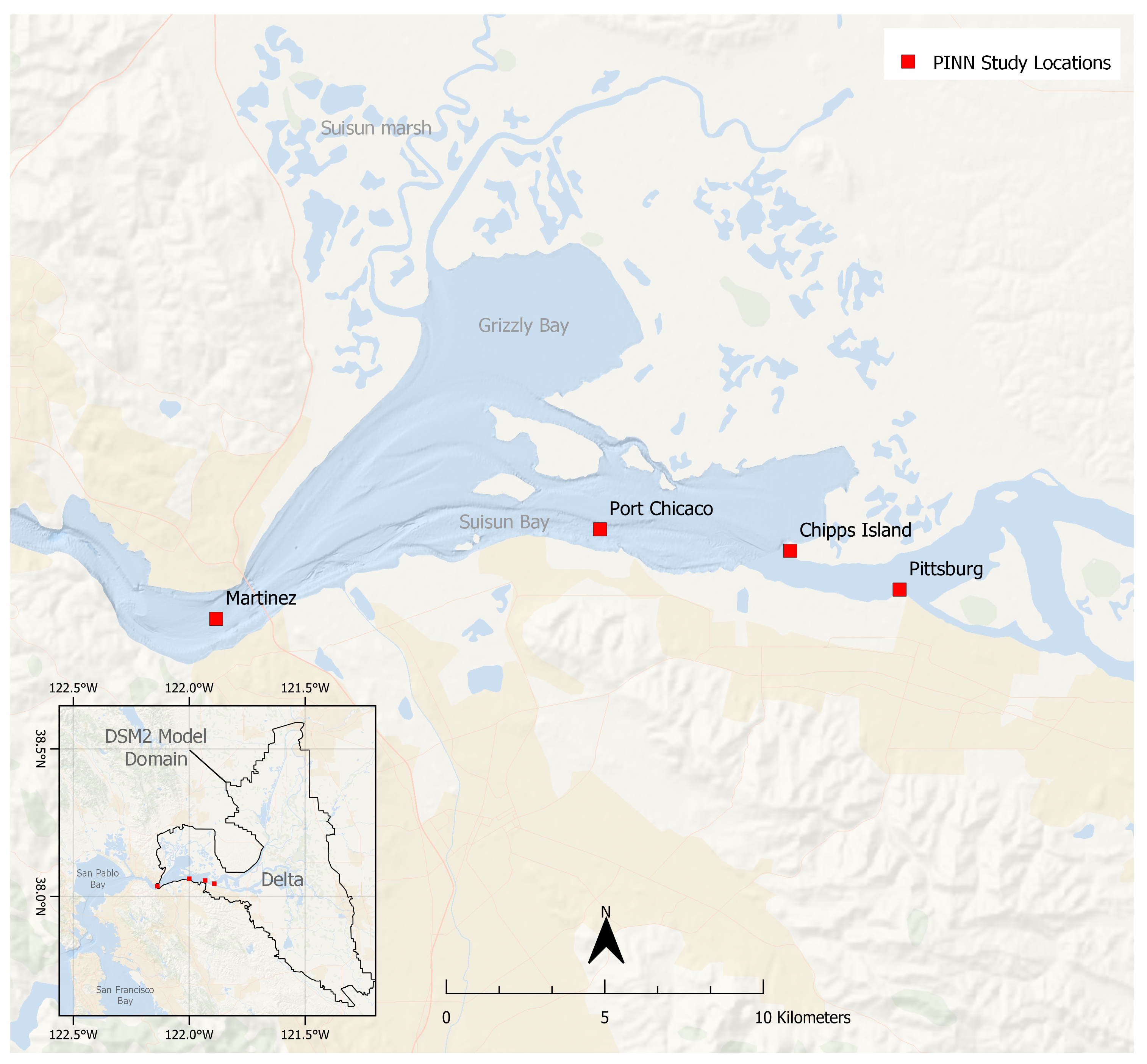
2.1. Study Locations and Dataset
2.2. Data Preprocessing
2.2.1. Normalization
2.2.2. Input Memory
2.3. Neural Network Architectures
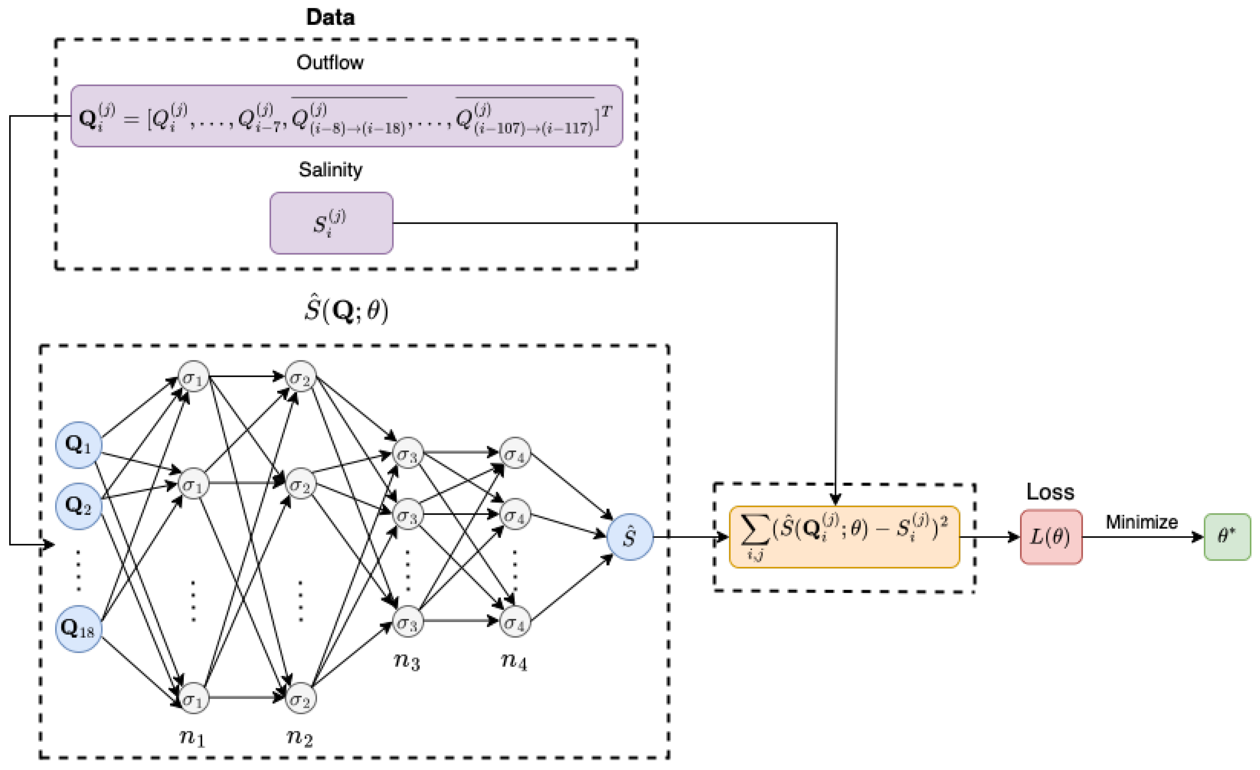
2.3.1. Artificial Neural Networks (ANN)
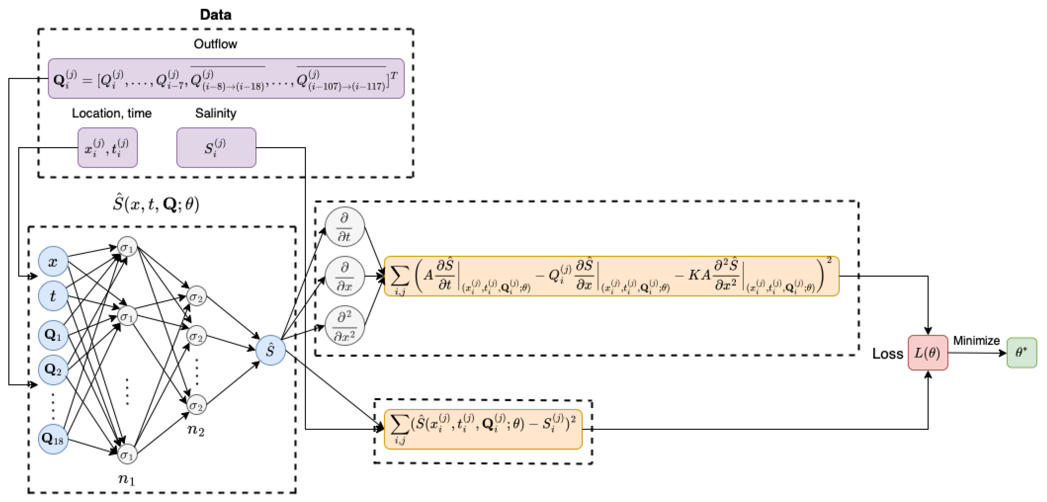
2.3.2. Physics-Informed Neural Networks (PINN)
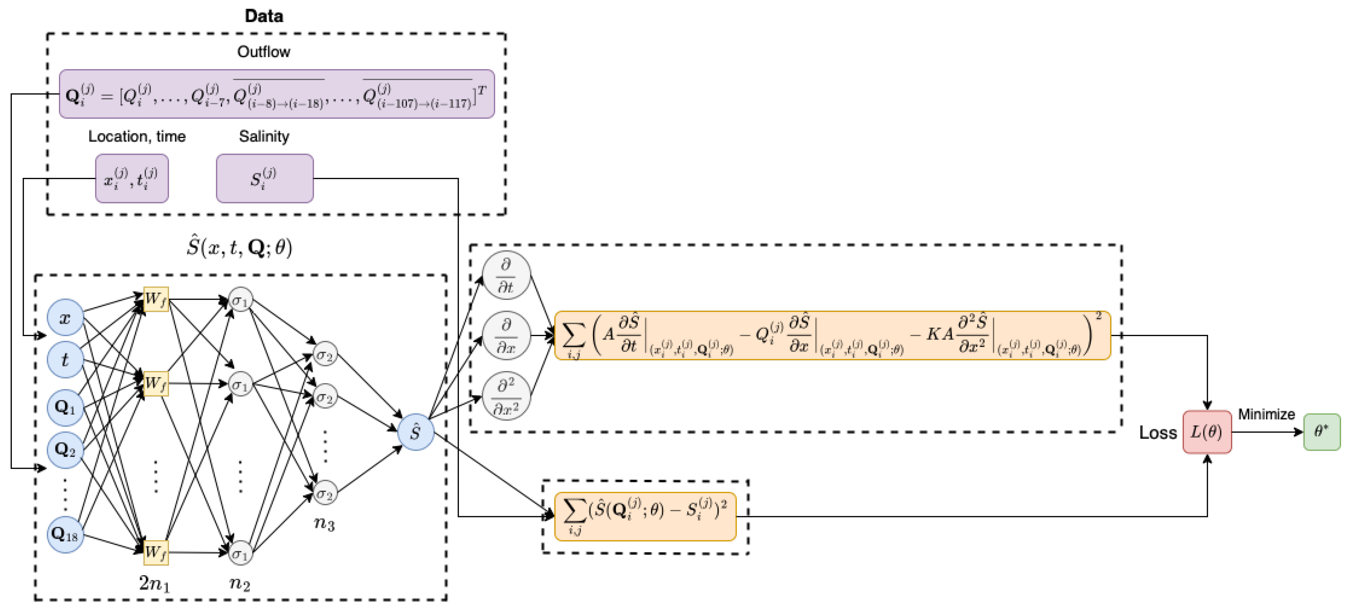
2.3.3. Physics-Informed Fourier Networks (FoNet)
2.4. Hyperparameter Search and Data Split
2.4.1. Hyperparameter Search
- ANN—the number of neurons in hidden layers 1 and 2, denoted as and , respectively, lie in the range of , and the number of neurons in hidden layer 3 and 4, denoted as and , lie in the range of .
- PINN— lies in the range of and lies in the range of .
- FoNet—, which represents the projection dimension size of the frequency matrix, lies in the range of , and and , the number of neurons in hidden layer 1 and 2, respectively, lie in the ranges of and , respectively.
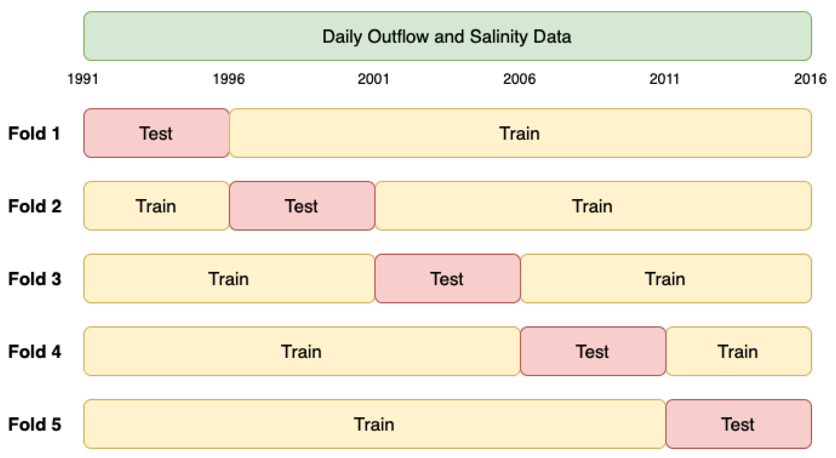
2.4.2. Data Split
2.5. Evaluation Metrics
2.6. Implementation Details
3. Results
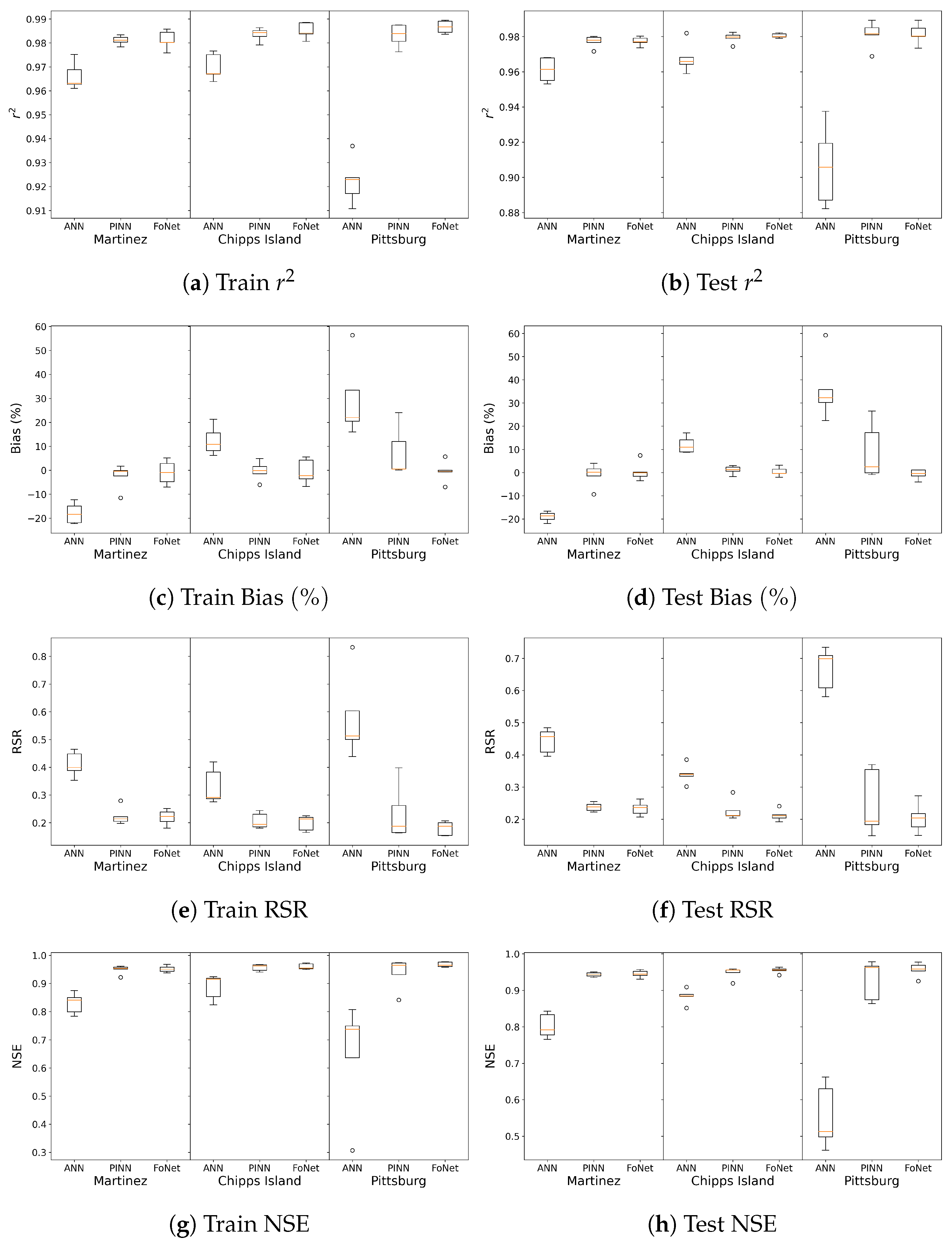
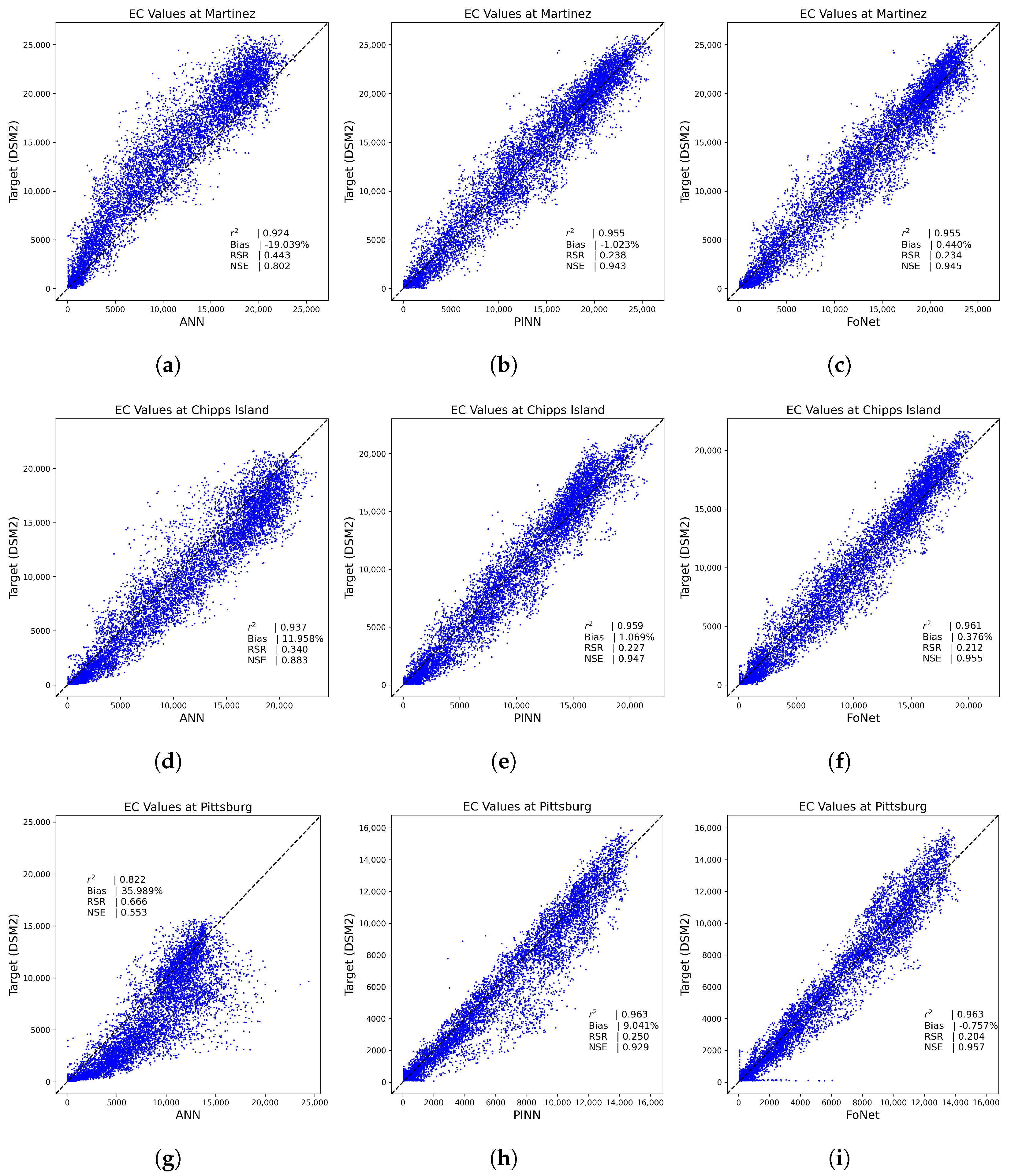
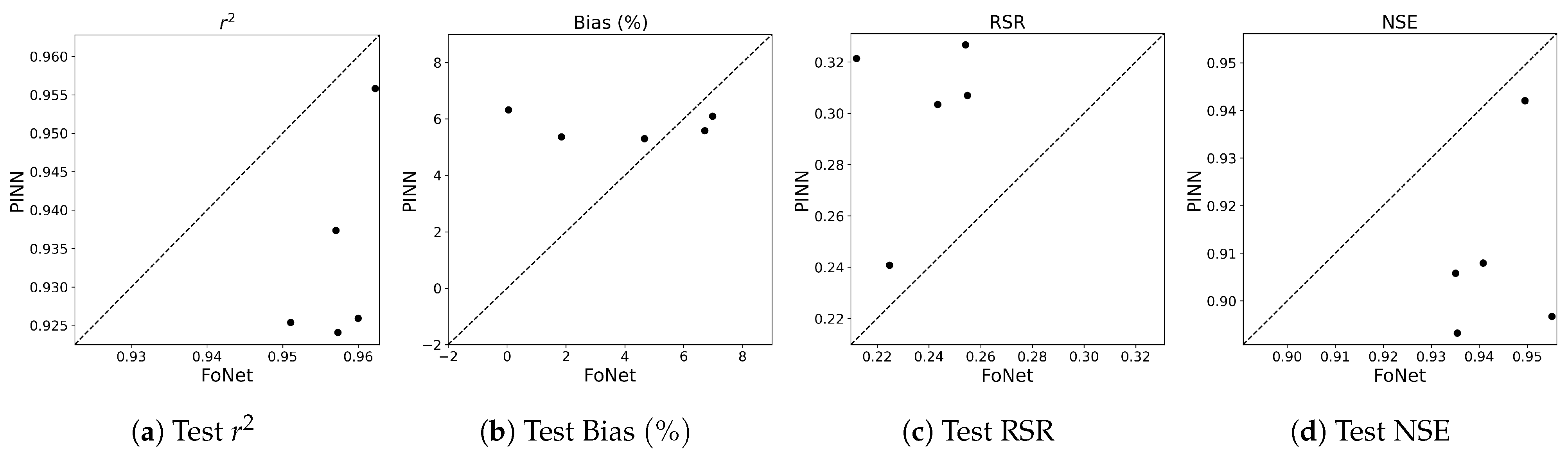
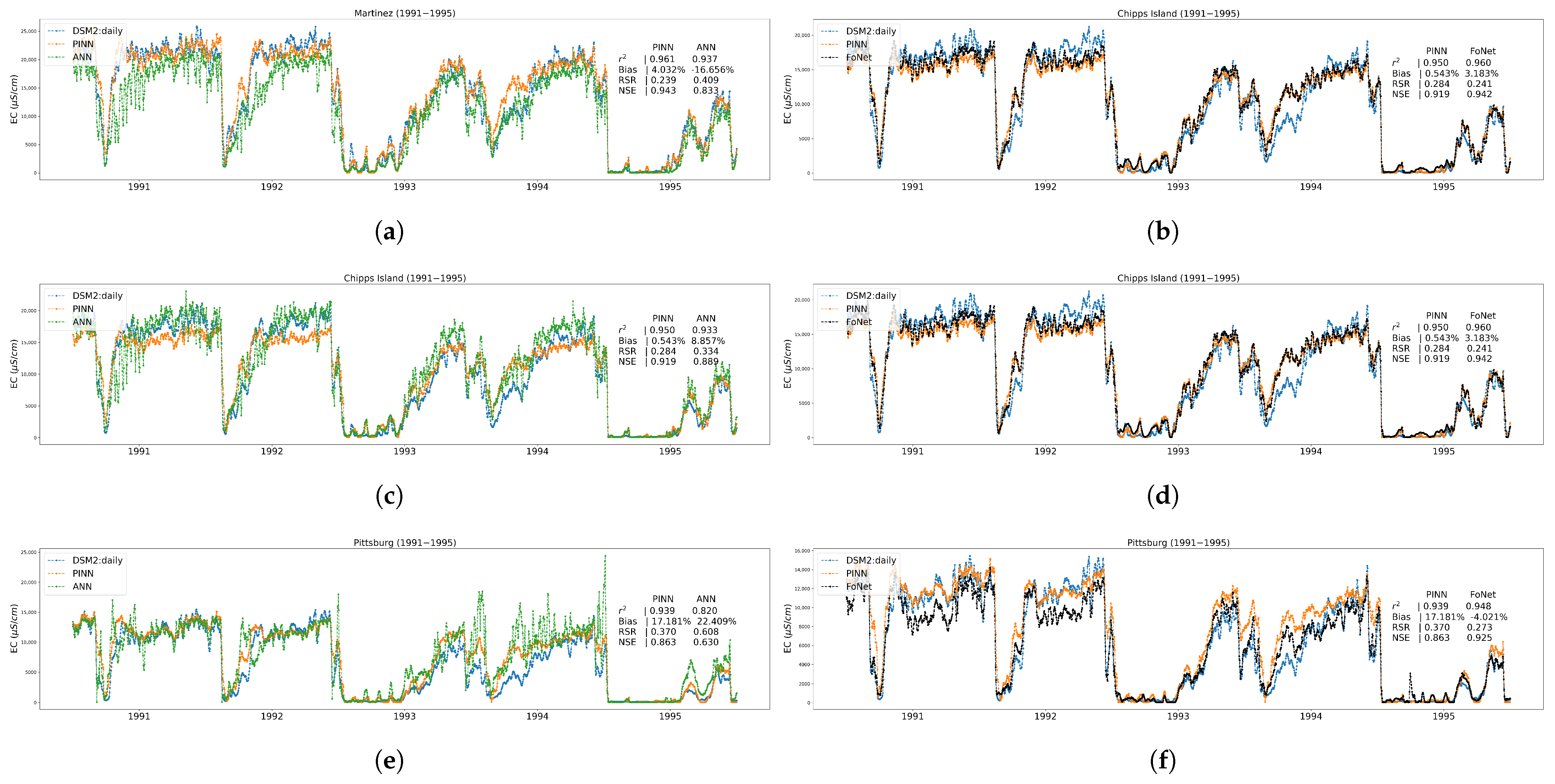
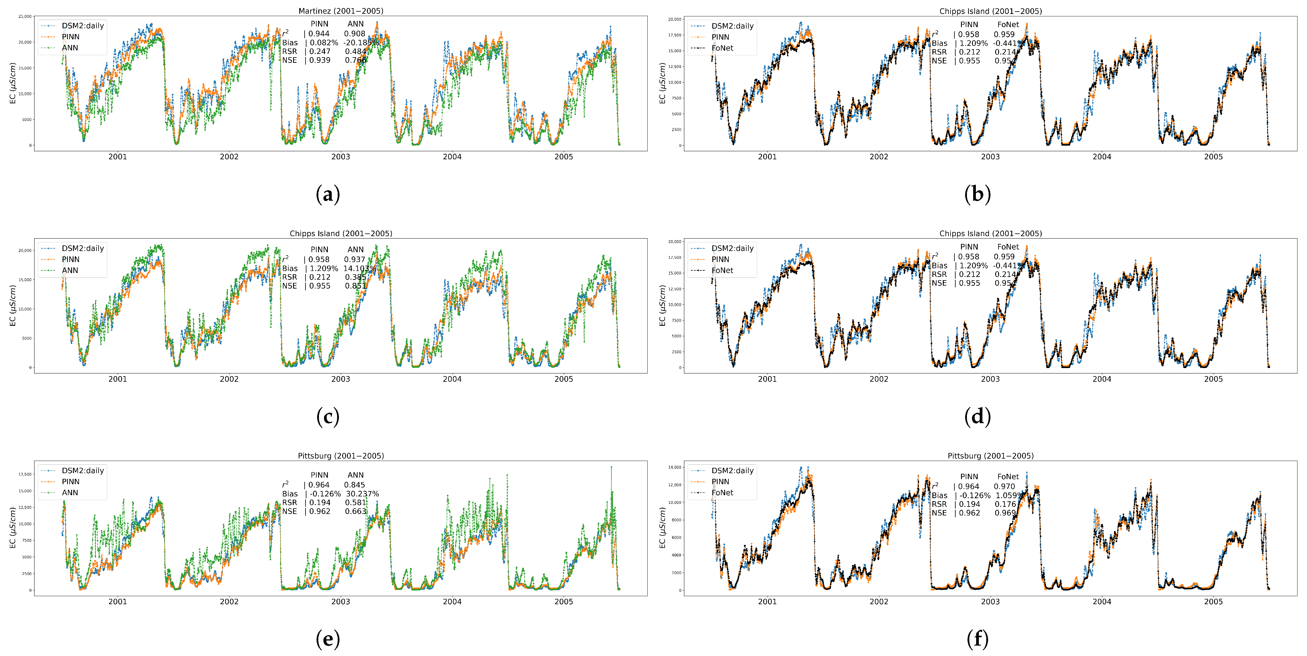
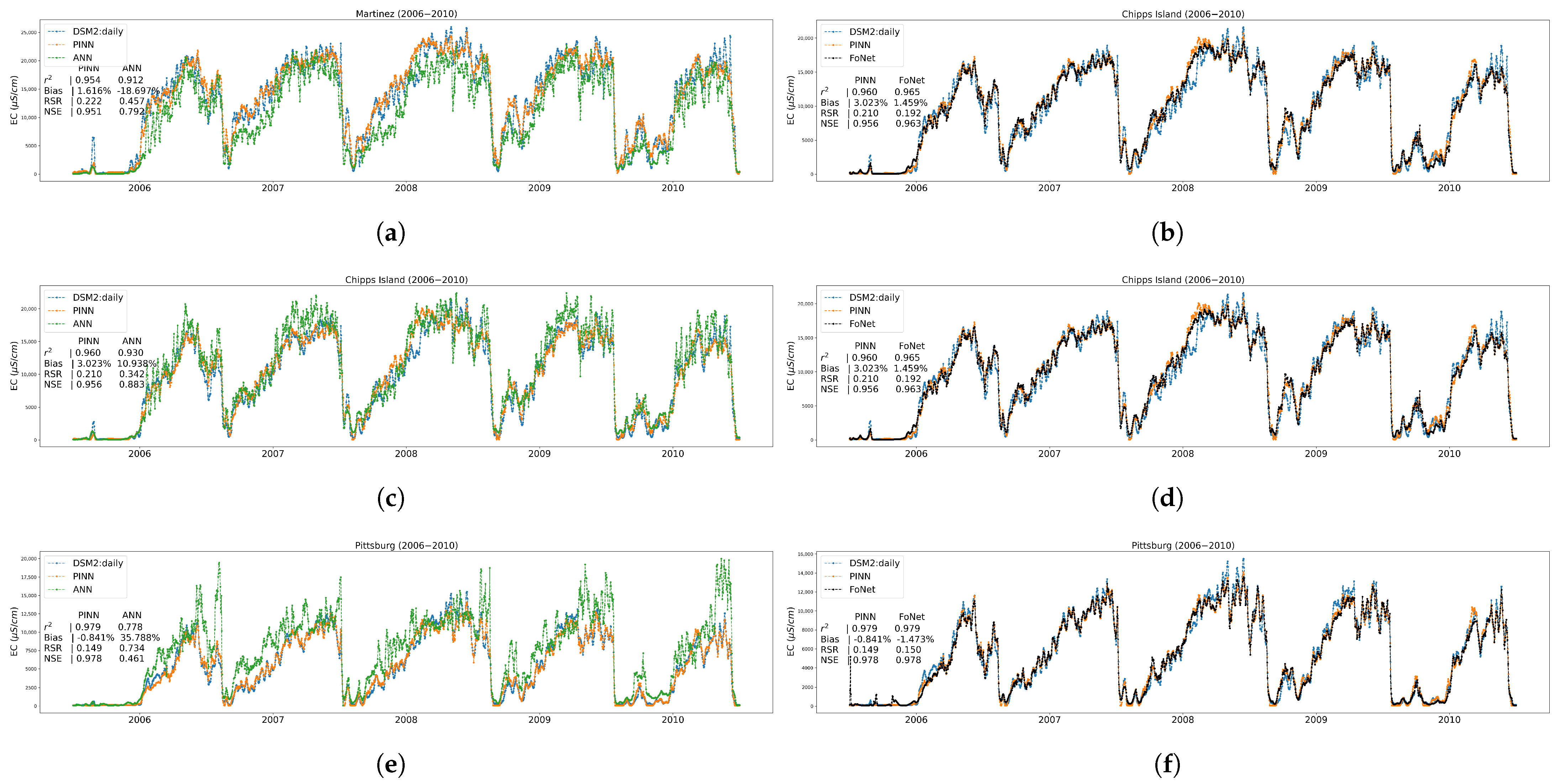
3.1. Performance Results on Trained Locations
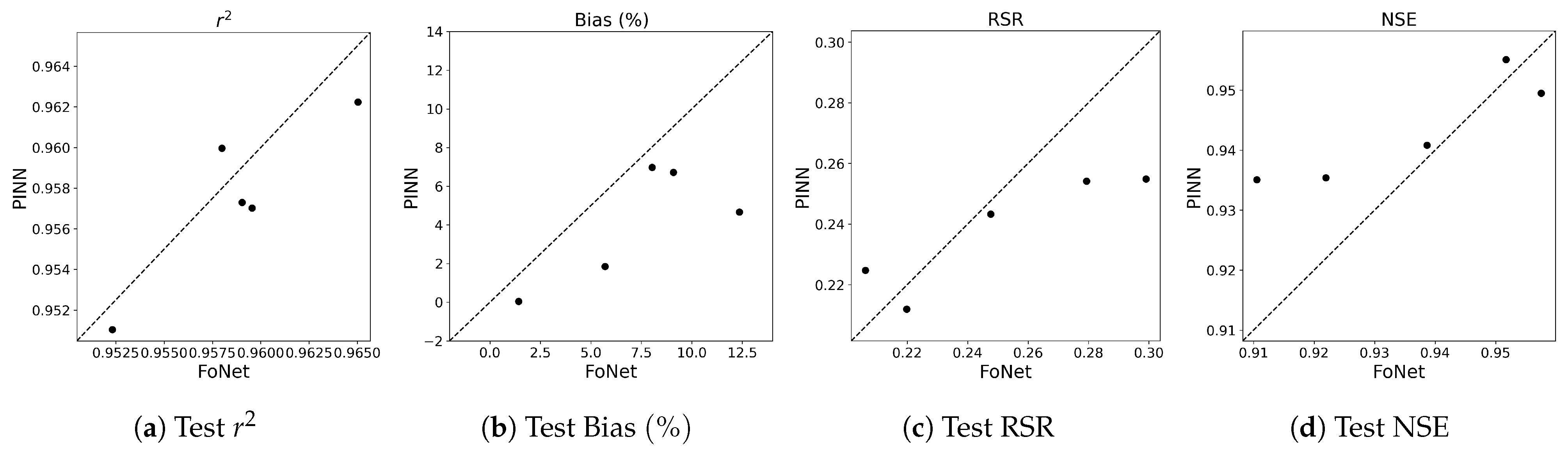
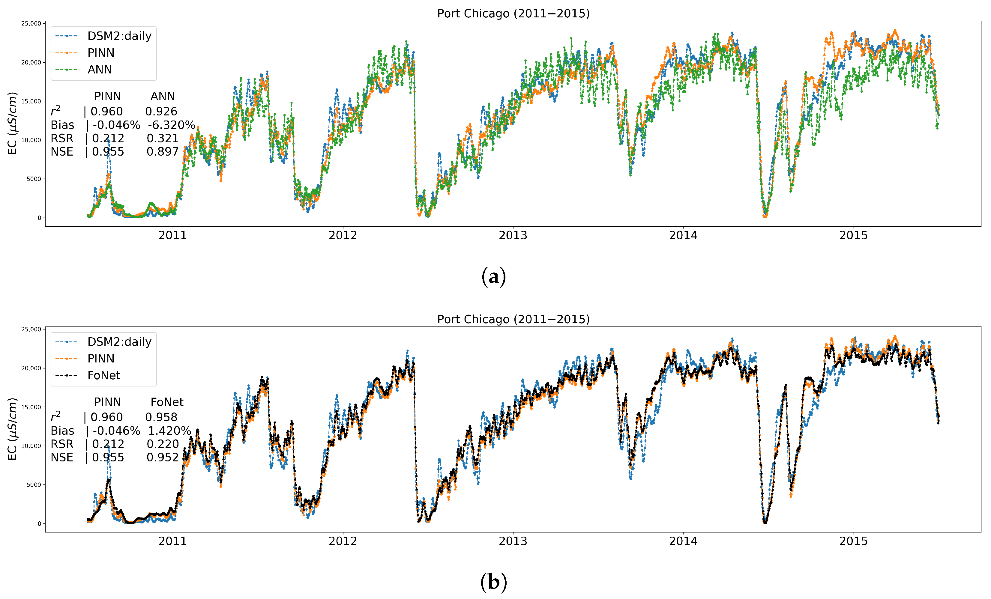
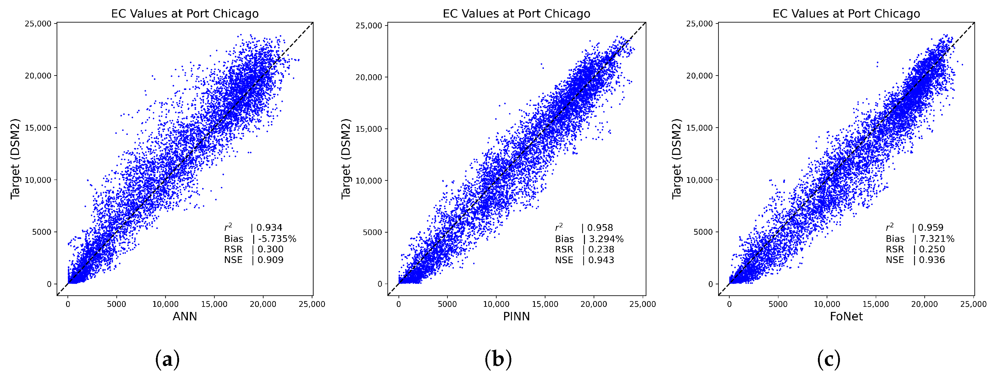
3.2. Performance Results on Independent Untrained Location
4. Discussion
4.1. Implications
4.2. Limitations and Future Work
5. Conclusions
Author Contributions
Funding
Data Availability Statement
Acknowledgments
Conflicts of Interest
Appendix A
Appendix A.1. ANN: Number of Layer Choices

| ANN | |||
|---|---|---|---|
| Evaluation Metrics | 2 Layers | 3 Layers | 4 Layers |
| 0.958 | 0.965 | 0.968 | |
| Bias | −6.491 | −6.242 | −5.302 |
| RSR | 0.338 | 0.313 | 0.307 |
| NSE | 0.886 | 0.902 | 0.906 |
Appendix A.2. Hyperparameter Choices
| Fold1 | Fold2 | Fold3 | Fold4 | Fold5 | ||||||
|---|---|---|---|---|---|---|---|---|---|---|
| Hidden Layer | # Neuron | Activation | # Neuron | Activation | # Neuron | Activation | # Neuron | Activation | # Neuron | Activation |
| hidden 1 | 32 | elu | 32 | relu | 32 | relu | 32 | tanh | 32 | relu |
| hidden 2 | 32 | elu | 8 | relu | 24 | relu | 24 | relu | 4 | tanh |
| hidden 3 | 8 | tanh | 14 | relu | 16 | elu | 2 | elu | 6 | elu |
| hidden 4 | 14 | sigmoid | 6 | tanh | 4 | sigmoid | 14 | relu | 12 | elu |
| Fold1 | Fold2 | Fold3 | Fold4 | Fold5 | ||||||
|---|---|---|---|---|---|---|---|---|---|---|
| Hidden Layer | # Neuron | Activation | # Neuron | Activation | # Neuron | Activation | # Neuron | Activation | # Neuron | Activation |
| hidden 1 | 24 | relu | 32 | relu | 24 | elu | 32 | tanh | 28 | tanh |
| hidden 2 | 12 | tanh | 16 | tanh | 12 | sigmoid | 16 | tanh | 8 | sigmoid |
| Fold1 | Fold2 | Fold3 | Fold4 | Fold5 | ||||||
|---|---|---|---|---|---|---|---|---|---|---|
| Hidden Layer | # Neuron | Activation | # Neuron | Activation | # Neuron | Activation | # Neuron | Activation | # Neuron | Activation |
| encoding | 24 | 28 | 32 | 16 | 8 | |||||
| hidden 1 | 32 | tanh | 16 | tanh | 12 | tanh | 28 | elu | 16 | tanh |
| hidden 2 | 10 | elu | 4 | sigmoid | 16 | relu | 8 | tanh | 10 | tanh |
Appendix A.3. Detailed Values for Box and Whisker Plots
| Fold1 | Fold2 | Fold3 | Fold4 | Fold5 | Average | |||||||||||||
|---|---|---|---|---|---|---|---|---|---|---|---|---|---|---|---|---|---|---|
| Station Name | ANN | PINN | FoNet | ANN | PINN | FoNet | ANN | PINN | FoNet | ANN | PINN | FoNet | ANN | PINN | FoNet | ANN | PINN | FoNet |
| Martinez | 0.938 | 0.961 | 0.961 | 0.927 | 0.957 | 0.952 | 0.951 | 0.967 | 0.972 | 0.923 | 0.963 | 0.969 | 0.928 | 0.965 | 0.961 | 0.933 | 0.963 | 0.963 |
| Port Chicago | 0.948 | 0.966 | 0.965 | 0.932 | 0.960 | 0.956 | 0.956 | 0.970 | 0.974 | 0.933 | 0.966 | 0.974 | 0.935 | 0.968 | 0.965 | 0.941 | 0.966 | 0.967 |
| Chipps Island | 0.951 | 0.966 | 0.968 | 0.929 | 0.959 | 0.962 | 0.954 | 0.973 | 0.977 | 0.935 | 0.969 | 0.977 | 0.935 | 0.970 | 0.968 | 0.941 | 0.967 | 0.970 |
| Pittsburg | 0.853 | 0.962 | 0.974 | 0.852 | 0.953 | 0.969 | 0.878 | 0.975 | 0.978 | 0.829 | 0.968 | 0.979 | 0.841 | 0.975 | 0.967 | 0.851 | 0.967 | 0.974 |
| Fold1 | Fold2 | Fold3 | Fold4 | Fold5 | Average | |||||||||||||
|---|---|---|---|---|---|---|---|---|---|---|---|---|---|---|---|---|---|---|
| Station Name | ANN | PINN | FoNet | ANN | PINN | FoNet | ANN | PINN | FoNet | ANN | PINN | FoNet | ANN | PINN | FoNet | ANN | PINN | FoNet |
| Martinez | 0.937 | 0.961 | 0.959 | 0.937 | 0.960 | 0.961 | 0.908 | 0.944 | 0.948 | 0.912 | 0.954 | 0.954 | 0.924 | 0.957 | 0.954 | 0.924 | 0.955 | 0.955 |
| Port Chicago | 0.937 | 0.957 | 0.960 | 0.956 | 0.962 | 0.965 | 0.925 | 0.951 | 0.952 | 0.924 | 0.957 | 0.959 | 0.926 | 0.960 | 0.958 | 0.934 | 0.958 | 0.959 |
| Chipps Island | 0.933 | 0.950 | 0.960 | 0.964 | 0.965 | 0.963 | 0.937 | 0.958 | 0.959 | 0.930 | 0.960 | 0.965 | 0.920 | 0.962 | 0.960 | 0.937 | 0.959 | 0.961 |
| Pittsburg | 0.820 | 0.939 | 0.948 | 0.879 | 0.962 | 0.961 | 0.845 | 0.964 | 0.970 | 0.778 | 0.979 | 0.979 | 0.787 | 0.970 | 0.960 | 0.822 | 0.963 | 0.963 |
| Fold1 | Fold2 | Fold3 | Fold4 | Fold5 | Average | |||||||||||||
|---|---|---|---|---|---|---|---|---|---|---|---|---|---|---|---|---|---|---|
| Station Name | ANN | PINN | FoNet | ANN | PINN | FoNet | ANN | PINN | FoNet | ANN | PINN | FoNet | ANN | PINN | FoNet | ANN | PINN | FoNet |
| Martinez | −21.874 | −11.528 | −6.950 | −14.911 | −0.411 | 5.117 | −18.398 | −0.163 | −0.957 | −22.276 | −2.386 | −4.792 | −12.369 | 1.730 | 2.825 | −17.966 | −2.552 | −0.952 |
| Port Chicago | −9.017 | −7.348 | −1.886 | −1.727 | 3.670 | 13.094 | −5.759 | 5.394 | 6.369 | −9.957 | 2.978 | 3.245 | 2.156 | 4.105 | 6.845 | −4.861 | 1.760 | 5.534 |
| Chipps Island | 8.201 | −6.066 | −6.773 | 15.562 | 4.887 | 4.238 | 10.801 | −0.191 | −2.297 | 6.214 | −1.454 | −3.619 | 21.264 | 1.520 | 5.597 | 12.408 | −0.261 | −0.571 |
| Pittsburg | 22.011 | 12.007 | −6.960 | 33.481 | 23.983 | −0.474 | 16.016 | 0.540 | 0.009 | 20.395 | 0.451 | −0.707 | 56.357 | 0.077 | 5.697 | 29.652 | 7.412 | −0.487 |
| Fold1 | Fold2 | Fold3 | Fold4 | Fold5 | Average | |||||||||||||
|---|---|---|---|---|---|---|---|---|---|---|---|---|---|---|---|---|---|---|
| Station Name | ANN | PINN | FoNet | ANN | PINN | FoNet | ANN | PINN | FoNet | ANN | PINN | FoNet | ANN | PINN | FoNet | ANN | PINN | FoNet |
| Martinez | −16.656 | 4.032 | 7.369 | −22.031 | −9.393 | −3.583 | −20.185 | 0.082 | 0.136 | −18.697 | 1.616 | −0.127 | −17.627 | −1.453 | −1.595 | −19.039 | −1.023 | 0.440 |
| Port Chicago | −5.302 | 4.666 | 12.357 | −5.369 | −1.848 | 5.702 | −5.585 | 6.715 | 9.091 | −6.101 | 6.982 | 8.034 | −6.320 | −0.046 | 1.420 | −5.735 | 3.294 | 7.321 |
| Chipps Island | 8.857 | 0.543 | 3.183 | 17.131 | 2.280 | −1.999 | 14.103 | 1.209 | −0.441 | 10.938 | 3.023 | 1.459 | 8.761 | −1.709 | −0.323 | 11.958 | 1.069 | 0.376 |
| Pittsburg | 22.409 | 17.181 | −4.021 | 59.230 | 26.537 | −0.388 | 30.237 | −0.126 | 1.059 | 35.788 | −0.841 | −1.473 | 32.283 | 2.453 | 1.040 | 35.989 | 9.041 | −0.757 |
| Fold1 | Fold2 | Fold3 | Fold4 | Fold5 | Average | |||||||||||||
|---|---|---|---|---|---|---|---|---|---|---|---|---|---|---|---|---|---|---|
| Station Name | ANN | PINN | FoNet | ANN | PINN | FoNet | ANN | PINN | FoNet | ANN | PINN | FoNet | ANN | PINN | FoNet | ANN | PINN | FoNet |
| Martinez | 0.448 | 0.279 | 0.239 | 0.399 | 0.222 | 0.251 | 0.388 | 0.197 | 0.181 | 0.465 | 0.214 | 0.205 | 0.353 | 0.205 | 0.223 | 0.411 | 0.224 | 0.220 |
| Port Chicago | 0.280 | 0.229 | 0.199 | 0.288 | 0.224 | 0.312 | 0.246 | 0.204 | 0.201 | 0.314 | 0.204 | 0.186 | 0.285 | 0.202 | 0.233 | 0.283 | 0.213 | 0.226 |
| Chipps Island | 0.276 | 0.231 | 0.225 | 0.383 | 0.244 | 0.219 | 0.286 | 0.181 | 0.165 | 0.291 | 0.194 | 0.173 | 0.419 | 0.185 | 0.213 | 0.331 | 0.207 | 0.199 |
| Pittsburg | 0.501 | 0.262 | 0.200 | 0.603 | 0.398 | 0.187 | 0.439 | 0.165 | 0.153 | 0.513 | 0.188 | 0.154 | 0.832 | 0.163 | 0.207 | 0.578 | 0.235 | 0.180 |
| Fold1 | Fold2 | Fold3 | Fold4 | Fold5 | Average | |||||||||||||
|---|---|---|---|---|---|---|---|---|---|---|---|---|---|---|---|---|---|---|
| Station Name | ANN | PINN | FoNet | ANN | PINN | FoNet | ANN | PINN | FoNet | ANN | PINN | FoNet | ANN | PINN | FoNet | ANN | PINN | FoNet |
| Martinez | 0.409 | 0.239 | 0.263 | 0.396 | 0.255 | 0.207 | 0.484 | 0.247 | 0.244 | 0.457 | 0.222 | 0.219 | 0.471 | 0.228 | 0.236 | 0.443 | 0.238 | 0.234 |
| Port Chicago | 0.307 | 0.255 | 0.299 | 0.241 | 0.225 | 0.206 | 0.327 | 0.254 | 0.279 | 0.303 | 0.243 | 0.248 | 0.321 | 0.212 | 0.220 | 0.300 | 0.238 | 0.250 |
| Chipps Island | 0.334 | 0.284 | 0.241 | 0.302 | 0.227 | 0.204 | 0.385 | 0.212 | 0.214 | 0.342 | 0.210 | 0.192 | 0.340 | 0.204 | 0.211 | 0.340 | 0.227 | 0.212 |
| Pittsburg | 0.608 | 0.370 | 0.273 | 0.708 | 0.355 | 0.217 | 0.581 | 0.194 | 0.176 | 0.734 | 0.149 | 0.150 | 0.698 | 0.183 | 0.204 | 0.666 | 0.250 | 0.204 |
| Fold1 | Fold2 | Fold3 | Fold4 | Fold5 | Average | |||||||||||||
|---|---|---|---|---|---|---|---|---|---|---|---|---|---|---|---|---|---|---|
| Station Name | ANN | PINN | FoNet | ANN | PINN | FoNet | ANN | PINN | FoNet | ANN | PINN | FoNet | ANN | PINN | FoNet | ANN | PINN | FoNet |
| Martinez | 0.799 | 0.922 | 0.943 | 0.841 | 0.951 | 0.937 | 0.850 | 0.961 | 0.967 | 0.784 | 0.954 | 0.958 | 0.875 | 0.958 | 0.950 | 0.830 | 0.949 | 0.951 |
| Port Chicago | 0.921 | 0.948 | 0.960 | 0.917 | 0.950 | 0.902 | 0.940 | 0.958 | 0.960 | 0.901 | 0.958 | 0.966 | 0.919 | 0.959 | 0.946 | 0.920 | 0.955 | 0.947 |
| Chipps Island | 0.924 | 0.947 | 0.949 | 0.853 | 0.940 | 0.952 | 0.918 | 0.967 | 0.973 | 0.916 | 0.962 | 0.970 | 0.824 | 0.966 | 0.955 | 0.887 | 0.957 | 0.960 |
| Pittsburg | 0.749 | 0.931 | 0.960 | 0.636 | 0.842 | 0.965 | 0.807 | 0.973 | 0.977 | 0.737 | 0.965 | 0.976 | 0.307 | 0.973 | 0.957 | 0.647 | 0.937 | 0.967 |
| Fold1 | Fold2 | Fold3 | Fold4 | Fold5 | Average | |||||||||||||
|---|---|---|---|---|---|---|---|---|---|---|---|---|---|---|---|---|---|---|
| Station Name | ANN | PINN | FoNet | ANN | PINN | FoNet | ANN | PINN | FoNet | ANN | PINN | FoNet | ANN | PINN | FoNet | ANN | PINN | FoNet |
| Martinez | 0.833 | 0.943 | 0.931 | 0.843 | 0.935 | 0.957 | 0.766 | 0.939 | 0.941 | 0.792 | 0.951 | 0.952 | 0.778 | 0.948 | 0.944 | 0.802 | 0.943 | 0.945 |
| Port Chicago | 0.906 | 0.935 | 0.911 | 0.942 | 0.950 | 0.958 | 0.893 | 0.935 | 0.922 | 0.908 | 0.941 | 0.939 | 0.897 | 0.955 | 0.952 | 0.909 | 0.943 | 0.936 |
| Chipps Island | 0.889 | 0.919 | 0.942 | 0.909 | 0.948 | 0.958 | 0.851 | 0.955 | 0.954 | 0.883 | 0.956 | 0.963 | 0.885 | 0.958 | 0.956 | 0.883 | 0.947 | 0.955 |
| Pittsburg | 0.630 | 0.863 | 0.925 | 0.498 | 0.874 | 0.953 | 0.663 | 0.962 | 0.969 | 0.461 | 0.978 | 0.978 | 0.512 | 0.966 | 0.958 | 0.553 | 0.929 | 0.957 |
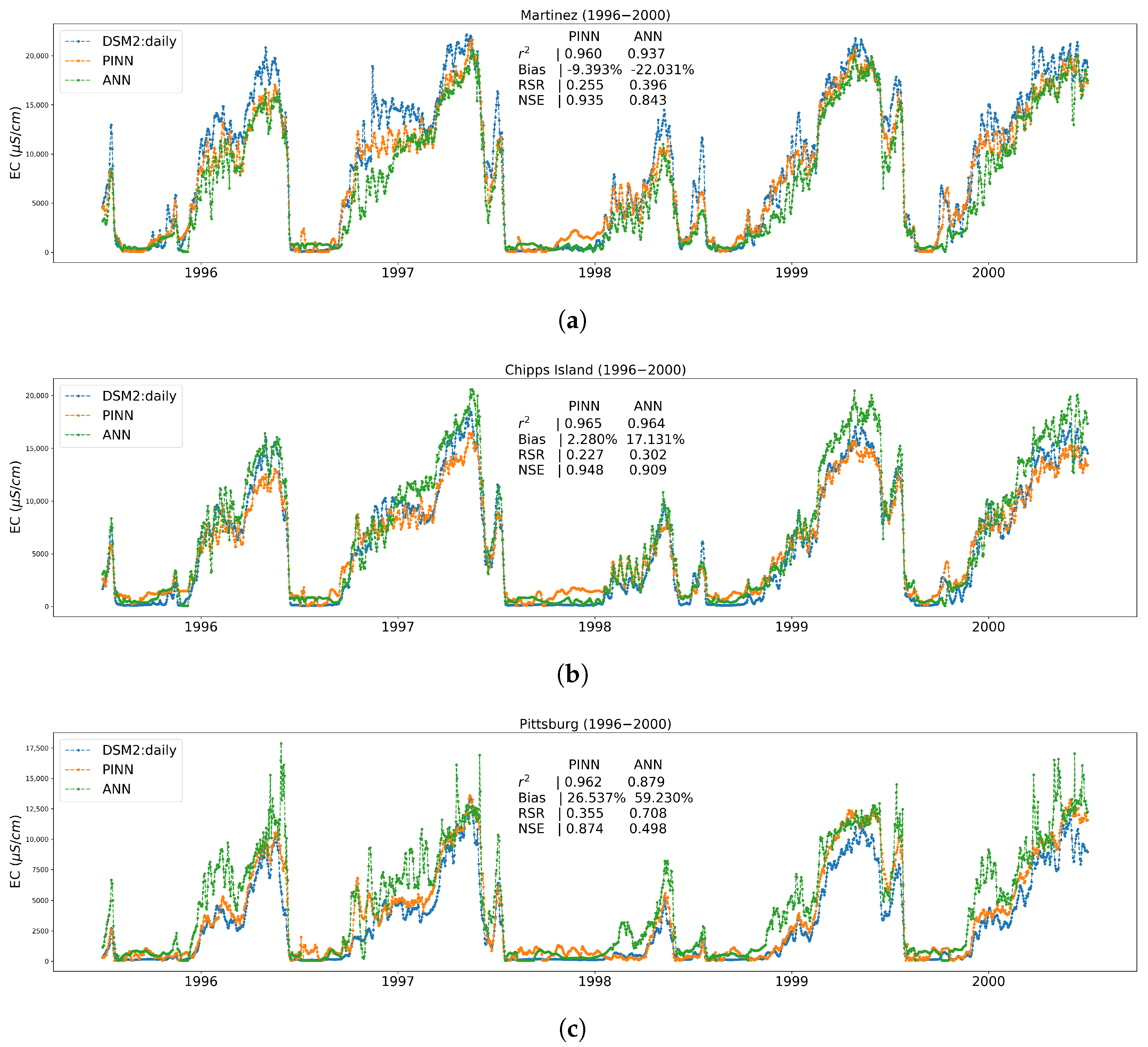
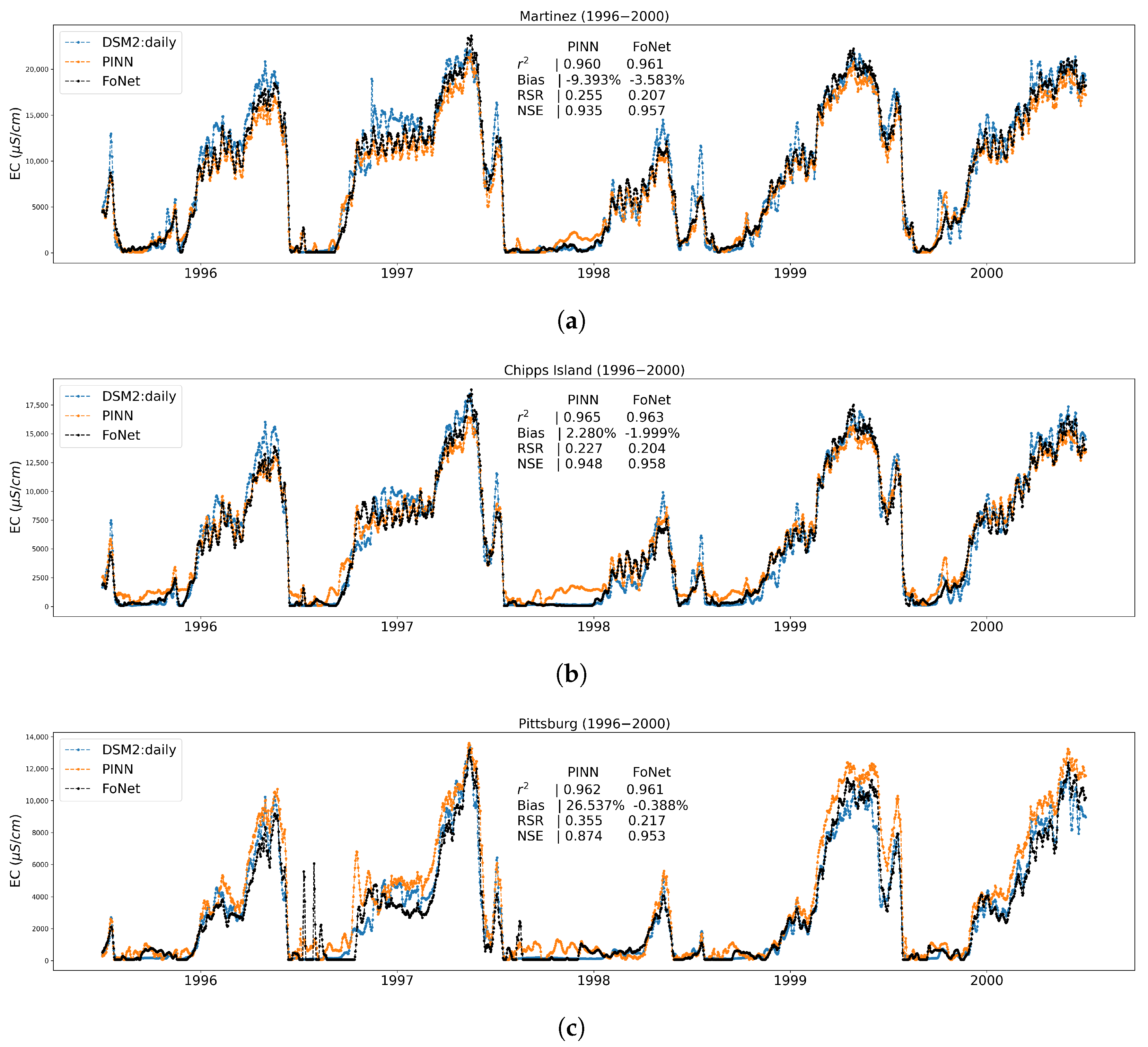
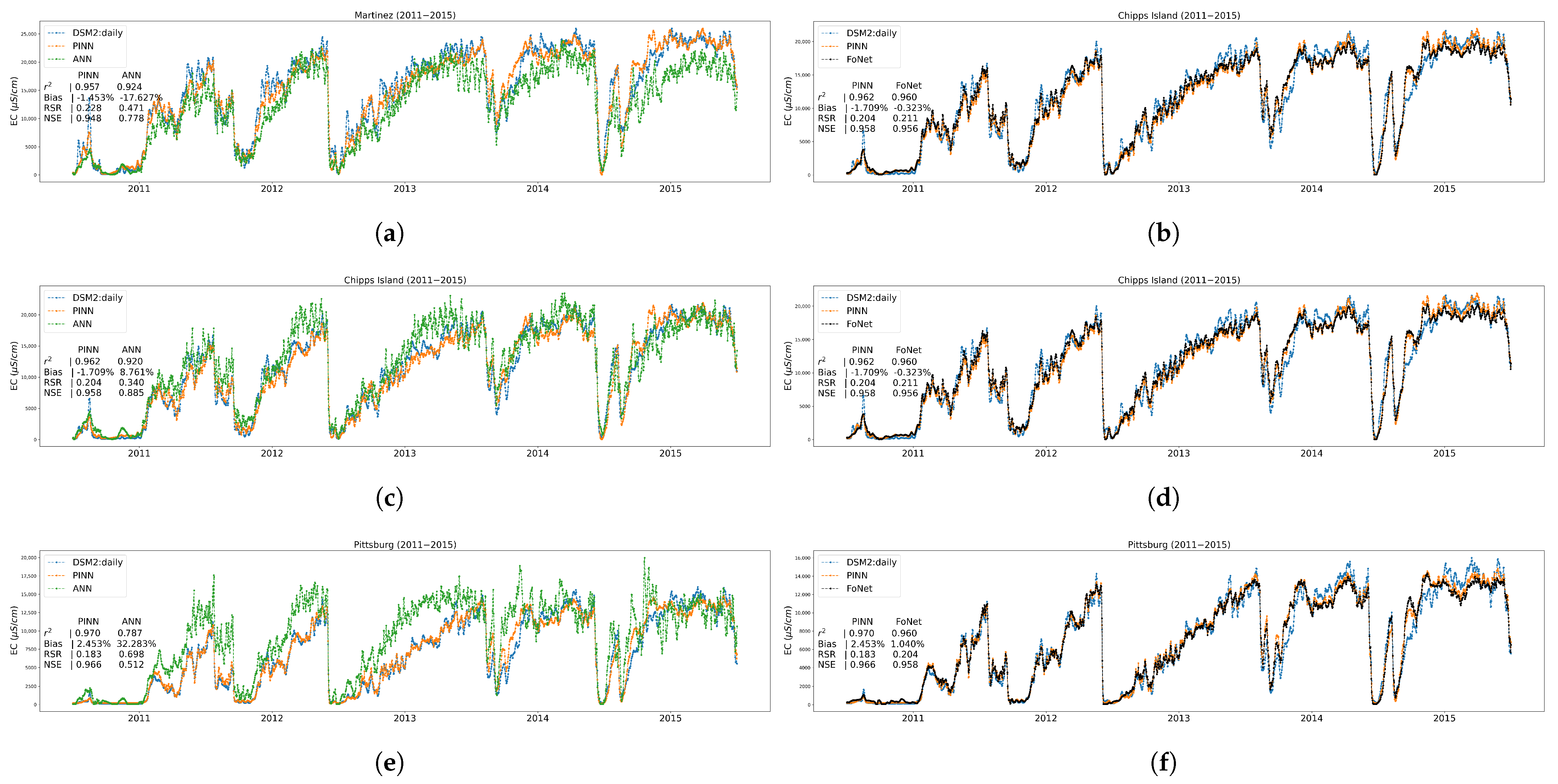
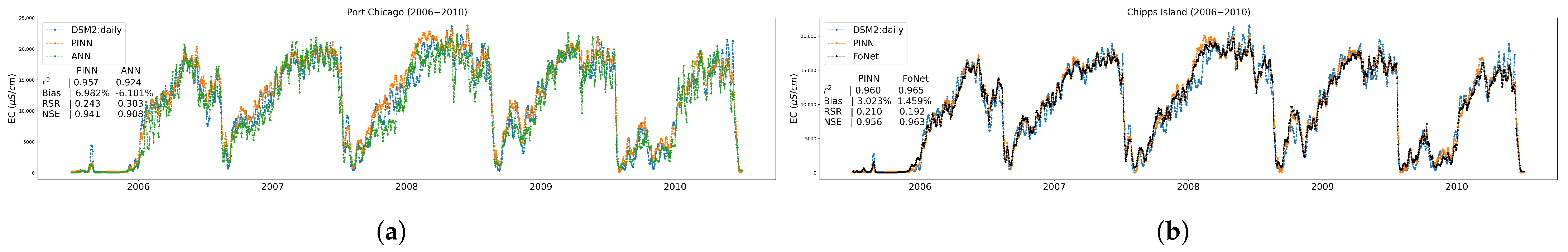
Appendix A.4. Time Series Plots at Three Trained Locations


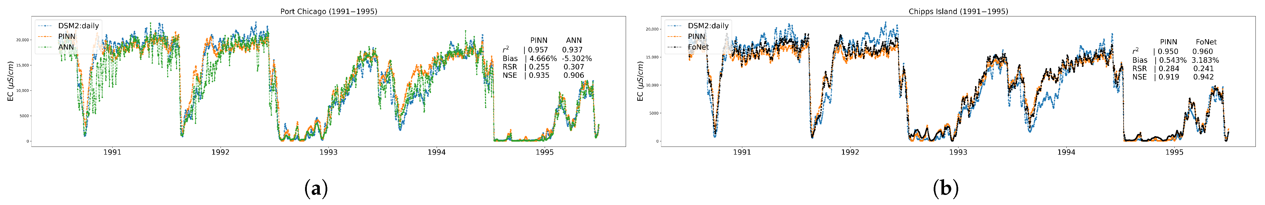
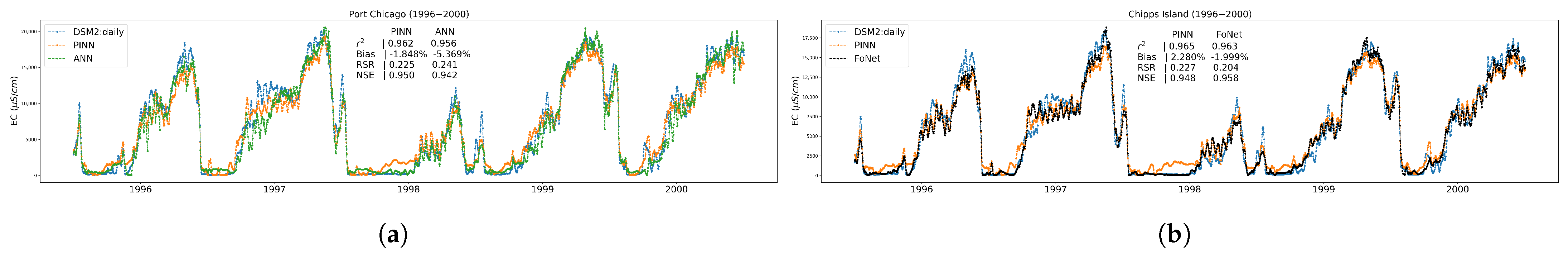
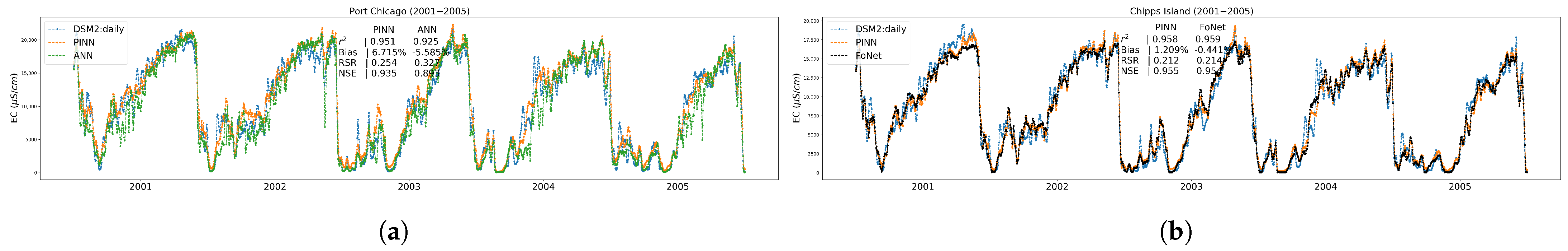
Appendix A.5. Time Series Plots at Port Chicago, an Independent Test Location


References
- Alber, M. A conceptual model of estuarine freshwater inflow management. Estuaries 2002, 25, 1246–1261. [Google Scholar] [CrossRef]
- Rath, J.S.; Hutton, P.H.; Chen, L.; Roy, S.B. A hybrid empirical-Bayesian artificial neural network model of salinity in the San Francisco Bay-Delta estuary. Environ. Model. Softw. 2017, 93, 193–208. [Google Scholar] [CrossRef]
- Xu, J.; Long, W.; Wiggert, J.D.; Lanerolle, L.W.; Brown, C.W.; Murtugudde, R.; Hood, R.R. Climate forcing and salinity variability in Chesapeake Bay, USA. Estuaries Coasts 2012, 35, 237–261. [Google Scholar] [CrossRef]
- Tran Anh, D.; Hoang, L.P.; Bui, M.D.; Rutschmann, P. Simulating future flows and salinity intrusion using combined one-and two-dimensional hydrodynamic modelling—The case of Hau River, Vietnamese Mekong delta. Water 2018, 10, 897. [Google Scholar] [CrossRef] [Green Version]
- Mulamba, T.; Bacopoulos, P.; Kubatko, E.J.; Pinto, G.F. Sea-level rise impacts on longitudinal salinity for a low-gradient estuarine system. Clim. Chang. 2019, 152, 533–550. [Google Scholar] [CrossRef]
- Doni, F.; Gasperini, A.; Soares, J.T. What is the SDG 13? In SDG13–Climate Action: Combating Climate Change and Its Impacts; Emerald Publishing Limited: Bingley, UK, 2020. [Google Scholar]
- Sadoff, C.W.; Borgomeo, E.; Uhlenbrook, S. Rethinking water for SDG 6. Nat. Sustain. 2020, 3, 346–347. [Google Scholar] [CrossRef]
- He, M.; Zhong, L.; Sandhu, P.; Zhou, Y. Emulation of a process-based salinity generator for the Sacramento–San Joaquin Delta of California via deep learning. Water 2020, 12, 2088. [Google Scholar] [CrossRef]
- Verruijt, A. A note on the Ghyben-Herzberg formula. Hydrol. Sci. J. 1968, 13, 43–46. [Google Scholar] [CrossRef]
- Todd, D.K.; Mays, L.W. Groundwater Hydrology; John Wiley & Sons: Hoboken, NJ, USA, 2004. [Google Scholar]
- Myers, N.; Mittermeier, R.A.; Mittermeier, C.G.; Da Fonseca, G.A.; Kent, J. Biodiversity hotspots for conservation priorities. Nature 2000, 403, 853–858. [Google Scholar] [CrossRef]
- Moyle, P.B.; Brown, L.R.; Durand, J.R.; Hobbs, J.A. Delta smelt: Life history and decline of a once-abundant species in the San Francisco Estuary. San Fr. Estuary Watershed Sci. 2016, 14. [Google Scholar] [CrossRef] [Green Version]
- CSWRCB. Water Right Decision 1641; CSWRCB: Sacramento, CA, USA, 1999; p. 225.
- USFWS. Formal Endangered Species Act Consultation on the Proposed Coordinated Operations of the Central Valley Project (CVP) and State Water Project (SWP); USFWS: Sacramento, CA, USA, 2008; p. 410.
- CDWR. Minimum Delta Outflow Program. In Methodology for Flow and Salinity Estimates in the Sacramento-San Joaquin Delta and Suisun Marsh: 11th Annual Progress Report; California Department of Water Resources: Sacramento, CA, USA, 1990. [Google Scholar]
- Denton, R.; Sullivan, G. Antecedent Flow-Salinity Relations: Application to Delta Planning Models. Contra Costa Water District Report 1993; p. 20. Available online: http://www.waterboards.ca.gov/waterrights/water_issues/programs/bay_delta/deltaflow/docs/exhibits/ccwd/spprt_docs/ccwd_denton_sullivan_1993.pdf (accessed on 1 April 2023).
- Denton, R.A. Accounting for antecedent conditions in seawater intrusion modeling—Applications for the San Francisco Bay-Delta. In Hydraulic Engineering; ASCE: Reston, VA, USA, 1993; pp. 448–453. [Google Scholar]
- CDWR. DSM2: Model Development. In Methodology for Flow and Salinity Estimates in the Sacramento-San Joaquin Delta and Suisun Marsh: 18th Annual Progress Report; California Department of Water Resources: Sacramento, CA, USA, 1997. [Google Scholar]
- Jayasundara, N.C.; Seneviratne, S.A.; Reyes, E.; Chung, F.I. Artificial neural network for Sacramento–San Joaquin Delta flow–salinity relationship for CalSim 3.0. J. Water Resour. Plan. Manag. 2020, 146, 04020015. [Google Scholar] [CrossRef]
- Wilbur, R.; Munevar, A. Integration of CALSIM and Artificial Neural Networks Models for Sacramento-San Joaquin Delta Flow-Salinity Relationships. In Methodology for Flow and Salinity Estimates in the Sacramento-San Joaquin Delta and Suisun Marsh: 22nd Annual Progress Report; California Department of Water Resources: Sacramento, CA, USA, 2001. [Google Scholar]
- Mierzwa, M. CALSIM versus DSM2 ANN and G-model Comparisons. In Methodology for Flow and Salinity Estimates in the Sacramento-San Joaquin Delta and Suisun Marsh: 23rd Annual Progress Report; California Department of Water Resources: Sacramento, CA, USA, 2002. [Google Scholar]
- Seneviratne, S.; Wu, S. Enhanced Development of Flow-Salinity Relationships in the Delta Using Artificial Neural Networks: Incorporating Tidal Influence. In Methodology for Flow and Salinity Estimates in the Sacramento-San Joaquin Delta and Suisun Marsh: 28th Annual Progress Report; California Department of Water Resources: Sacramento, CA, USA, 2007. [Google Scholar]
- CDWR. Calibration and verification of DWRDSM. In Methodology for Flow and Salinity Estimates in the Sacramento-San Joaquin Delta and Suisun Marsh: 12th Annual Progress Report; California Department of Water Resources: Sacramento, CA, USA, 1991. [Google Scholar]
- Chen, L.; Roy, S.B.; Hutton, P.H. Emulation of a process-based estuarine hydrodynamic model. Hydrol. Sci. J. 2018, 63, 783–802. [Google Scholar] [CrossRef]
- Cheng, R.T.; Casulli, V.; Gartner, J.W. Tidal, residual, intertidal mudflat (TRIM) model and its applications to San Francisco Bay, California. Estuar. Coast. Shelf Sci. 1993, 36, 235–280. [Google Scholar] [CrossRef]
- DeGeorge, J.F. A Multi-Dimensional Finite Element Transport Model Utilizing a Characteristic-Galerkin Algorithm; University of California: Davis, CA, USA, 1996. [Google Scholar]
- MacWilliams, M.; Bever, A.J.; Foresman, E. 3-D simulations of the San Francisco Estuary with subgrid bathymetry to explore long-term trends in salinity distribution and fish abundance. San Fr. Estuary Watershed Sci. 2016, 14. [Google Scholar] [CrossRef] [Green Version]
- Chao, Y.; Farrara, J.D.; Zhang, H.; Zhang, Y.J.; Ateljevich, E.; Chai, F.; Davis, C.O.; Dugdale, R.; Wilkerson, F. Development, implementation, and validation of a modeling system for the San Francisco Bay and Estuary. Estuar. Coast. Shelf Sci. 2017, 194, 40–56. [Google Scholar] [CrossRef]
- Qi, S.; He, M.; Bai, Z.; Ding, Z.; Sandhu, P.; Zhou, Y.; Namadi, P.; Tom, B.; Hoang, R.; Anderson, J. Multi-Location Emulation of a Process-Based Salinity Model Using Machine Learning. Water 2022, 14, 2030. [Google Scholar] [CrossRef]
- MacWilliams, M.L.; Ateljevich, E.S.; Monismith, S.G.; Enright, C. An overview of multi-dimensional models of the Sacramento–San Joaquin Delta. San Fr. Estuary Watershed Sci. 2016, 14. [Google Scholar] [CrossRef] [Green Version]
- Gopi, A.; Sharma, P.; Sudhakar, K.; Ngui, W.K.; Kirpichnikova, I.; Cuce, E. Weather Impact on Solar Farm Performance: A Comparative Analysis of Machine Learning Techniques. Sustainability 2023, 15, 439. [Google Scholar] [CrossRef]
- Sharma, P.; Bora, B.J. A Review of Modern Machine Learning Techniques in the Prediction of Remaining Useful Life of Lithium-Ion Batteries. Batteries 2022, 9, 13. [Google Scholar] [CrossRef]
- Barnes, G.W., Jr.; Chung, F.I. Operational planning for California water system. J. Water Resour. Plan. Manag. 1986, 112, 71–86. [Google Scholar] [CrossRef]
- Draper, A.J.; Munévar, A.; Arora, S.K.; Reyes, E.; Parker, N.L.; Chung, F.I.; Peterson, L.E. CalSim: Generalized model for reservoir system analysis. J. Water Resour. Plan. Manag. 2004, 130, 480–489. [Google Scholar] [CrossRef]
- Qi, S.; Bai, Z.; Ding, Z.; Jayasundara, N.; He, M.; Sandhu, P.; Seneviratne, S.; Kadir, T. Enhanced Artificial Neural Networks for Salinity Estimation and Forecasting in the Sacramento-San Joaquin Delta of California. J. Water Resour. Plan. Manag. 2021, 147, 04021069. [Google Scholar] [CrossRef]
- Qi, S.; He, M.; Bai, Z.; Ding, Z.; Sandhu, P.; Chung, F.; Namadi, P.; Zhou, Y.; Hoang, R.; Tom, B.; et al. Novel Salinity Modeling Using Deep Learning for the Sacramento–San Joaquin Delta of California. Water 2022, 14, 3628. [Google Scholar] [CrossRef]
- Shen, C.; Appling, A.P.; Gentine, P.; Bandai, T.; Gupta, H.; Tartakovsky, A.; Baity-Jesi, M.; Fenicia, F.; Kifer, D.; Li, L.; et al. Differentiable modeling to unify machine learning and physical models and advance Geosciences. arXiv 2023, arXiv:2301.04027. [Google Scholar]
- Daw, A.; Thomas, R.Q.; Carey, C.C.; Read, J.S.; Appling, A.P.; Karpatne, A. Physics-guided architecture (pga) of neural networks for quantifying uncertainty in lake temperature modeling. In Proceedings of the 2020 Siam International Conference on Data Mining, Cincinnati, OH, USA, 7–9 May 2020; pp. 532–540. [Google Scholar]
- Hoedt, P.J.; Kratzert, F.; Klotz, D.; Halmich, C.; Holzleitner, M.; Nearing, G.S.; Hochreiter, S.; Klambauer, G. Mc-lstm: Mass-conserving lstm. In Proceedings of the International Conference on Machine Learning, Virtual Event, 18–24 July 2021; pp. 4275–4286. [Google Scholar]
- Bertels, D.; Willems, P. Physics-informed machine learning method for modelling transport of a conservative pollutant in surface water systems. J. Hydrol. 2023, 619, 129354. [Google Scholar] [CrossRef]
- Feng, D.; Liu, J.; Lawson, K.; Shen, C. Differentiable, Learnable, Regionalized Process-Based Models With Multiphysical Outputs can Approach State-Of-The-Art Hydrologic Prediction Accuracy. Water Resour. Res. 2022, 58, e2022WR032404. [Google Scholar] [CrossRef]
- Raissi, M.; Perdikaris, P.; Karniadakis, G.E. Physics-informed neural networks: A deep learning framework for solving forward and inverse problems involving nonlinear partial differential equations. J. Comput. Phys. 2019, 378, 686–707. [Google Scholar] [CrossRef]
- Psichogios, D.C.; Ungar, L.H. A hybrid neural network-first principles approach to process modeling. AIChE J. 1992, 38, 1499–1511. [Google Scholar] [CrossRef]
- Cuomo, S.; Di Cola, V.S.; Giampaolo, F.; Rozza, G.; Raissi, M.; Piccialli, F. Scientific machine learning through physics–informed neural networks: Where we are and what’s next. J. Sci. Comput. 2022, 92, 88. [Google Scholar] [CrossRef]
- Cedillo, S.; Núñez, A.G.; Sánchez-Cordero, E.; Timbe, L.; Samaniego, E.; Alvarado, A. Physics-Informed Neural Network water surface predictability for 1D steady-state open channel cases with different flow types and complex bed profile shapes. Adv. Model. Simul. Eng. Sci. 2022, 9, 1–23. [Google Scholar] [CrossRef]
- Yang, Y.; Mei, G. A Deep Learning-Based Approach for a Numerical Investigation of Soil–Water Vertical Infiltration with Physics-Informed Neural Networks. Mathematics 2022, 10, 2945. [Google Scholar] [CrossRef]
- Bishop, C.M.; Nasrabadi, N.M. Pattern Recognition and Machine Learning; Springer: Berlin, Germany, 2006; Volume 4. [Google Scholar]
- Anderson, J. DSM2 fingerprinting technology. In Methodology for Flow and Salinity Estimates in the Sacramento-San Joaquin Delta and Suisun Marsh: 23rd Annual Progress Report; California Department of Water Resources: Sacramento, CA, USA, 2002. [Google Scholar]
- Sandhu, N.; Finch, R. Application of artificial neural networks to the Sacramento-San Joaquin Delta. In Proceedings of the Estuarine and Coastal Modeling; ASCE: Reston, VA, USA, 1995; pp. 490–504. [Google Scholar]
- Sanskrityayn, A.; Suk, H.; Chen, J.S.; Park, E. Generalized analytical solutions of the advection-dispersion equation with variable flow and transport coefficients. Sustainability 2021, 13, 7796. [Google Scholar] [CrossRef]
- Rumelhart, D.E.; Hinton, G.E.; Williams, R.J. Learning representations by back-propagating errors. Nature 1986, 323, 533–536. [Google Scholar] [CrossRef]
- Rahaman, N.; Baratin, A.; Arpit, D.; Draxler, F.; Lin, M.; Hamprecht, F.; Bengio, Y.; Courville, A. On the spectral bias of neural networks. In Proceedings of the International Conference on Machine Learning, Long Beach, CA, USA, 10–15 June 2019; pp. 5301–5310. [Google Scholar]
- Mildenhall, B.; Srinivasan, P.P.; Tancik, M.; Barron, J.T.; Ramamoorthi, R.; Ng, R. Nerf: Representing scenes as neural radiance fields for view synthesis. Commun. ACM 2021, 65, 99–106. [Google Scholar] [CrossRef]
- Tancik, M.; Srinivasan, P.; Mildenhall, B.; Fridovich-Keil, S.; Raghavan, N.; Singhal, U.; Ramamoorthi, R.; Barron, J.; Ng, R. Fourier features let networks learn high frequency functions in low dimensional domains. Adv. Neural Inf. Process. Syst. 2020, 33, 7537–7547. [Google Scholar]
- Snijders, T.A. On cross-validation for predictor evaluation in time series. In Proceedings of the On Model Uncertainty and its Statistical Implications: Proceedings of a Workshop, Groningen, The Netherlands, 25–26 September 1986; Springer: Berlin, Germany, 1988; pp. 56–69. [Google Scholar]
- Montgomery, D.C.; Peck, E.A.; Vining, G.G. Introduction to Linear Regression Analysis; John Wiley & Sons: Hoboken, NJ, USA, 2021. [Google Scholar]
- Legates, D.R.; McCabe, G.J., Jr. Evaluating the use of “goodness-of-fit” measures in hydrologic and hydroclimatic model validation. Water Resour. Res. 1999, 35, 233–241. [Google Scholar] [CrossRef]
- Gupta, H.V.; Kling, H.; Yilmaz, K.K.; Martinez, G.F. Decomposition of the mean squared error and NSE performance criteria: Implications for improving hydrological modelling. J. Hydrol. 2009, 377, 80–91. [Google Scholar] [CrossRef] [Green Version]
- Nash, J.E.; Sutcliffe, J.V. River flow forecasting through conceptual models part I—A discussion of principles. J. Hydrol. 1970, 10, 282–290. [Google Scholar] [CrossRef]
- Kingma, D.P.; Ba, J. Adam: A method for stochastic optimization. arXiv 2014, arXiv:1412.6980. [Google Scholar]
- Wang, S.; Wang, H.; Perdikaris, P. On the eigenvector bias of Fourier feature networks: From regression to solving multi-scale PDEs with physics-informed neural networks. Comput. Methods Appl. Mech. Eng. 2021, 384, 113938. [Google Scholar] [CrossRef]


| Name | Definition | Formula |
|---|---|---|
| Squared Correlation Coefficient | ||
| Bias | Percent Bias | |
| RSR | RMSE-observations standard deviation ratio | |
| NSE | Nash–Sutcliffe Efficiency coefficient |
Disclaimer/Publisher’s Note: The statements, opinions and data contained in all publications are solely those of the individual author(s) and contributor(s) and not of MDPI and/or the editor(s). MDPI and/or the editor(s) disclaim responsibility for any injury to people or property resulting from any ideas, methods, instructions or products referred to in the content. |
© 2023 by the authors. Licensee MDPI, Basel, Switzerland. This article is an open access article distributed under the terms and conditions of the Creative Commons Attribution (CC BY) license (https://creativecommons.org/licenses/by/4.0/).
Share and Cite
Roh, D.M.; He, M.; Bai, Z.; Sandhu, P.; Chung, F.; Ding, Z.; Qi, S.; Zhou, Y.; Hoang, R.; Namadi, P.; et al. Physics-Informed Neural Networks-Based Salinity Modeling in the Sacramento–San Joaquin Delta of California. Water 2023, 15, 2320. https://0-doi-org.brum.beds.ac.uk/10.3390/w15132320
Roh DM, He M, Bai Z, Sandhu P, Chung F, Ding Z, Qi S, Zhou Y, Hoang R, Namadi P, et al. Physics-Informed Neural Networks-Based Salinity Modeling in the Sacramento–San Joaquin Delta of California. Water. 2023; 15(13):2320. https://0-doi-org.brum.beds.ac.uk/10.3390/w15132320
Chicago/Turabian StyleRoh, Dong Min, Minxue He, Zhaojun Bai, Prabhjot Sandhu, Francis Chung, Zhi Ding, Siyu Qi, Yu Zhou, Raymond Hoang, Peyman Namadi, and et al. 2023. "Physics-Informed Neural Networks-Based Salinity Modeling in the Sacramento–San Joaquin Delta of California" Water 15, no. 13: 2320. https://0-doi-org.brum.beds.ac.uk/10.3390/w15132320