
Non-Equilibrium Bedload Transport Model Applied to Erosive Overtopping Dambreach

1
Fluid Dynamic Technologies I3A, University of Zaragoza, C. Maria de Luna 3, 50018 Zaragoza, Spain
2
Estación Experimental Aula Dei EEAD, CSIC, Avda. Montañana 1005, 50059 Zaragoza, Spain
*
Author to whom correspondence should be addressed.
Water 2023, 15(17), 3094; https://0-doi-org.brum.beds.ac.uk/10.3390/w15173094
Submission received: 8 August 2023
/
Revised: 23 August 2023
/
Accepted: 26 August 2023
/
Published: 29 August 2023
(This article belongs to the Special Issue Advances in Dam-Break Modeling for Flood Hazard Mitigation: Theory, Numerical Models, and Applications in Hydraulic Engineering)
Abstract
:Bedload sediment transport is an ubiquitous process in natural surface water flows (rivers, dams, coast, etc), but it also plays a key role in catastrophic events such as dyke erosion or dam breach collapse. The bedload transport mechanism can be under equilibrium state, where solid rate and flow carry capacity are balanced, or under non-equilibrium (non-capacity) conditions. Extremely transient surface flows, such as dam/dyke erosive collapses, are systems which always change in space and time, hence absolute equilibrium states in the coupled fluid/solid transport rarely exist. Intuitively, assuming non-equilibrium conditions in transient flows should allow to estimate correctly the bedload transport rates and the bed level evolution. To get insight into this topic, a 2D Finite Volume model for bedload transport based on the non-capacity approach is proposed in this work. This non-equilibrium model considers that the actual bedload sediment discharge can be delayed, spatial and temporally, from the instantaneous solid carry capacity of the flow. Furthermore, the actual solid rate and the adaptation length/time is governed by the temporal evolution of the bedload transport layer and the vertical exchange solid flux. The model is tested for the simulation of overtopping dyke erosion and dambreach opening cases. Numerical results seems to support that considering non-equilibrium conditions for the bedload transport improves the general agreement between the computed results and measured data in both benchmarking cases.
1. Introduction
In surface water flows, such as river or coasts, the bed material particles are transported by two main mechanisms: suspended load transport accounts for the sediment particles moving within the flow column, whereas bedload transport involves the particles moving in a relatively thin layer over the static bed stratum. In this bedload transport layer, the solid particles are in contact with the underlying static stratum and hence the particle velocity is much lower than that of the the surrounding fluid [1]. The bedload transport plays a key role in the riverbed morphology since it can lead to marked and rapid variations in the bed level. Bedload transport can occur under a steady equilibrium state or, contrarily, under transient non-equilibrium conditions. The classical equilibrium approach considers that the actual bedload rate is the capacity of the flow to carry solid weight and hence only depending on instantaneous local flow features. The capacity bedload rate can be estimated using different empirical closure relations found in literature [2] and is the most widespread approach in current bedload transport models [3,4,5,6,7,8,9,10].
Contrarily, in bedload models based on the non-equilibrium assumption, the actual transport rates must be computed through the advection of the solid particles in the bedload layer and the mass exchange with the underlying static riverbed [11,12,13,14,15], and usually it does not agree with the local load carry capacity of the flow. Intuitively, assuming non-equilibrium conditions in transient flows should allow to estimate correctly the solid transport rates and the bed evolution, but this topic remains uncertain nowadays. Van-Rijn [16] suggested that the bedload rate can be assumed equal to the solid carry capacity event in moderate unsteady flows, since the adjustment of the transported solid load to new local flow conditions proceeds enough rapid close to the riverbed surface. However, this assumption was only conceptual and not supported by theoretical or numerical results. Later, analysing numerically the time scale of the processes involved in bedload transport, Cao et al. [13,17] found that the bedload rate was able adapt rapidly to the local carry capacity in flood cases. These works seem to justify the widespread application of the equilibrium/capacity bedload models [17]. However, this fact is not supported by any results in case of highly transient erosive dambreach flows.
Assuming non-equilibrium conditions for the bedload transport requires to compute locally both the thickness of the bedload transport layer and the bulk velocity of the solid particles. Furthermore, the net exchange flux of solid particles between static riverbed and moving bedload layer also has to be estimated, since it works as a source/sink of solid load. Therefore, non-equilibrium bedload models for transient flows involve a high uncertainty in the estimation of the parameters associated to entrainment/deposition vertical flux and the transport layer thickness and velocity. In the specialized literature, different strategies have been reported to overcome this uncertainty. El Kadi Abderrezzak et al. [18] assumed non-storage conditions for the transport layer and approximated the net solid flux through the interface between the static bed and the moving transport layer by the divergence between the actual and capacity transport rates. This theoretical model also introduced the adaptation length concept, fixed in time and space, leading to the quasi-steady relaxation flux approach for bedload models. Based on the same adaptation length concept, refs. [11,19,20] proposed more complex approaches to determine the net exchange flux through the interface but accounting now for the mass storage in the bedload transport layer. These models assume the actual transport rate as one of the unknown conservative variables, but they estimate the bulk bedload layer velocity using the closure relations found in literature [21,22,23] developed in laboratory under solid carry capacity conditions.
Recently, novel complex developments applying the non-capacity approach in bedload transport models have been derived, most of them based on the pioneering work Charru [24]. This work studies, at a grain scale, the mechanical interaction between moving fluid (clear water) and sediment particles at the interface between the static riverbed and the moving bedload layer. Based on this particle-scale momentum balance, Zech et al. [25] modelled the net exchange flux through the interface as a function of the shear stress exerted by the flow in the bedload transport layer and the shear strength for the incipient motion at the upper boundary of the static underlying stratum. Based also on [24], Fernández-Nieto et al. [14,26] derived closure relationships for the erosion and deposition rates at the static-moving interface, leading to a novel expression for the actual solid transport rate under non-equilibrium conditions. Under equilibrium conditions, this new expression for the solid transport reduces to the classical formula for bedload rate. Some interesting works have been recently published modelling bedload transport rates in cohesive clay–silt–gravel mixtures [27,28]. Finally, Bohorquez and Ancey [15] performed a grain-scale analysis of the particle activity at the bedload transport layer and proposed expressions for the entrainment/deposition rates including an additional diffusion term in the non-capacity bedload transport equation.
In this work, the novel generalized non-equilibrium bedload transport formulation developed by Martínez-Aranda et al. [29,30] for 2D bedload transport models is used to simulate dyke overtopping erosion and dam breach collapse processes. The equilibrium and non-equilibrium approaches are compared for different synthetic tests and experimental benchmarking cases. The main goal of this work is to test the suitability of the non-equilibrium approach for these highly unsteady erosive flows. This manuscript organized as follows: in Section 2 the system of conservation equations for 2D bedload transport is introduced; the numerical method is detailed in Section 3; the model results for one synthetic test and two experimental benchmarking cases are analysed in Section 4; and finally the main conclusions are drawn in Section 5.
2. Mathematical Modelling of 2D Generalized Bedload Transport
The 2D governing equations for bedload transport assuming non-equilibrium approach can be written as a compact conservation laws system [30], which includes the conservation laws for the water mass and the depth-averaged momentum of the flow, together with the transport equation for the erodible bed material:
where are the conservative variables, and are the conservative fluxes along the x- and y-coordinates respectively:
being h the flow depth, ( the components of the depth-averaged velocity along the x- and y-coordinates respectively, is the erodible bed elevation, are the components of the non-equilibrium bedload discharge along the x- and y-coordinates respectively and g is the gravity acceleration. On the right hand side, the terms includes the bed-pressure momentum source and accounts for the frictional momentum dissipation along the x- and y-coordinates:
being the components of the boundary shear stress vector between the flow and the movable bed along the x- and y-coordinates, respectively, and () the corresponding frictional energy loss. For the sake of simplicity, in this work the turbulent Manning friction formulation is adopted:
where is the depth-averaged flow velocity modulus and n is the bulk Manning roughness parameter depending on the bed material.
The bedload solid discharge in classical morpho-dynamical models is considered under equilibrium (capacity) conditions and usually modelled using the Grass law [31], which scales exponentially the solid transport rate with the flow velocity as , being a flow-bed interaction constant factor and m an behaviour exponent (usually ). More complex equilibrium models applied to realistic bedload transport tests estimate the instantaneous local flow-bed interaction factor from the hydro-dynamical flow features, hence [2,10,32], being the dimensionless Shields stress at the bed surface. According to Martínez-Aranda et al. [29] and Martínez-Aranda et al. [30], the bedload transport rate assuming a non-equilibrium approach can be expressed following a modified Grass-type law as:
being the bed layer porosity and G a interaction factor between the flow and erodible riverbed. This interaction factor depends not only on the flow depth h and the dimensionless Shields stress , but also on the bedload transport layer thickness . Figure 1 shows a schematic representation of the bedload generalized bedload mechanism at grain-scale.
It is useful to split G in a product of three factors , and as:
Table 1 provides expressions for functions , and using empirical relations found in literature, where is the relative density of the sediment particles , is the characteristic diameter of the bed sediment, and are the two constants associated to the deposition and erosion exchange rates, respectively, between the underlying static bed stratum and the bedload transport layer (moving layer). The term accounts for the excess of Shields stress over the critical threshold for the incipient motion threshold of the solid particles, calculated as:
This generalized Grass-type model (6) allows to consider capacity (equilibrium) or non-equilibrium approaches for the bedload transport only by selecting the proper estimation procedure for the bedload layer thickness . On one hand, assuming the equilibrium approach leads to the instantaneous adaptation of the bedload transport rate to its capacity value and the equilibrium transport layer thickness can be estimated as:
On the other hand, the non-equilibrium assumption forces the necessity of estimating the temporal evolution of the bedload transport layer thickness using the conservation equation:
where and are the entrainment and deposition vertical rates, respectively, between the the underlying static stratum and the bedload transport layer. Following [24,29], the volumetric entrainment and deposition rates can be expressed as:
3. Numerical Scheme for the 2D Bedload Transport Model
In order to obtain the numerical solution applying Finite Volume (FV) methods, the spatial domain is discretized into a fixed-in-time mesh of triangular cells and system (1) is integrated in each computational cell using the Gauss theorem:
being the inner domain and the number of edges for the i cell, the outward unit normal vector and the length of the kth edge. Assuming a piecewise representation of the conservative variables at each i cell, , the updating formulation between from time to the next step is expressed as:
where is the i cell area, is the time step, is the inverse of the rotation matrix at kth edge [33] and is the numerical normal flux throughout the kth edge. This numerical normal flux includes the convective flux augmented with the non-conservative bed-pressure contribution and the frictional momentum dissipation integrated thought the edge.
In this work, the upwind computation of is achieved using a fully-coupled Roe-type Riemann solver for bedload transport (FCM solver) [34]. This augmented 5-waves solver is based on computing the approximated solution of the linear Riemann problem:
where denotes the normal axis to the cell edge and superscripts ˜ indicates edge-averaged quantities. The pseudo-Jacobian matrix of the coupled system includes the approximated Jacobian matrix of the conservative convective flux and the non-conservative matrix of the bed-pressure momentum contribution at the edge. On the right hand side, the term denotes the momentum dissipation due to flow-bed frictional stress, integrated through the kth edge. Details on the flux computation have been extensively reported in Martínez-Aranda et al. [34] but, for the sake of brevity, at the kth edge is computed as:
where are the wave celerities at the edge, i.e., the eigenvalues of the pseudo-Jacobian matrix whereas are the corresponding eigenvectors. The coefficients denotes the wave strengths which accounts for the discontinuity on the conservative variables, whereas the coefficients are the source strengths involving the frictional momentum contribution at the edge. The subscript under the sums indicate that only the waves travelling inward the i cell are considered, leading to the upwind computation of the flux at the edge.
Furthermore, the stability of the explicitly computed numerical solution is addressed by the dynamical limitation of the global time step using a CFL condition. The local time step allowed for the kth edge is estimated assuming that the absolute maximum of the eigenvalues corresponds to the fastest wave celerity. Hence the global time step is limited by minimum of the local time steps, i.e., the more restrictive instantaneous local flow features (see Martínez-Aranda et al. [34]).
3.1. Transport Layer Updating with Capacity and Non-Capacity Approaches
Once the conservative variables have been updated using (12), the bedload transport rate is computed at the next time level as:
where the hydrodynamic quantities , , and are directly extracted from . Nevertheless, Equation (15) also requires to compute the updated bedload transport layer thickness at the next time level. The updating of the transport layer thickness depends on the assumption made for the bedload transport:
- Equilibrium hypothesis: The new transport layer thickness is directly computed as:where is the Shields excess (7) at the i cell computed from the updated conservative variables .
- Non-capacity approach: This leads to the necessity of solving Equation (9) each time step. The updating formula for the transport layer thickness is expressed as:being the numerical normal flux at the kth intercell edge for the transport layer equation and and the values of the entrainment and deposition rates for the i cell at time n, respectively. To compute the numerical flux , the bedload transport layer Equation (9) is projected along the normal direction to the edge and approximated by the local scalar Riemann problem:where the virtual bedload wave celerity is defined as:being and , and the bedload numerical flux is computed as:The cell-centered exchange rates and between the underlying static stratum and the transport layer are computed as:
3.2. Morphological Collapse Mechanism
In realistic applications, the maximum bed level slope is limited due to morphological collapse processes. In order to implement an efficient bed slope control mechanism, we propose the non-iterative limitation of the numerical beload flux provided for the augmented Riemann solver at each cell edge imposing geometrical restrictions. The bed level updating expressions for the left L and right R cells sharing the edge read:
where and refer to the non-shared edges of the left and right cells respectively and denotes the forth component of the numerical flux vector at the common edge between cells L and R. This value is provided by the Riemann solver, i.e., the numerical upwind bedload normal flux at the edge (). Therefore, the evolution of the local bed slope at edge can be expressed as:
Assuming a collapse bed slope angle along the edge-normal distance between cell centres , two conditions arise for the morphological limiting of the numerical bedload flux depending on the sign of the local bed slope:
- Positive bed slope if
- Negative bed slope if
Actually, this limitation on the numerical bedload flux acts as a bed form control mechanism, including artificial diffusion in the numerical bed level solution and avoiding the appearance of shock waves in the bed level with local slopes larger than the morphological collapse limit.
4. Numerical Results and Discussion
4.1. Adaptation of the Non-Equilibrium Bedload Rate to Equilibrium States
This new generalised model for the non-equilibrium bedload transport (5)–(6) requires to compute the thickness of the transport layer using (9), but it is able to account for the spatial and temporal delay of the actual bedload rate with respect to the solid transport capacity in highly unsteady flows. Moreover, if the local flow features allow to develop steady states in the bedload transport process, the entrainment and deposition rates tend to balance () and the solid rate recovers the equilibrium condition, characterized by the transport layer thickness (8). Therefore, the equilibrium state is a particular case of the generalised non-equilibrium model where .
In order to illustrate the temporal-spatial behaviour of the generalised non-equilibrium bedload model, a simple idealised test is included here forcing the following flow conditions
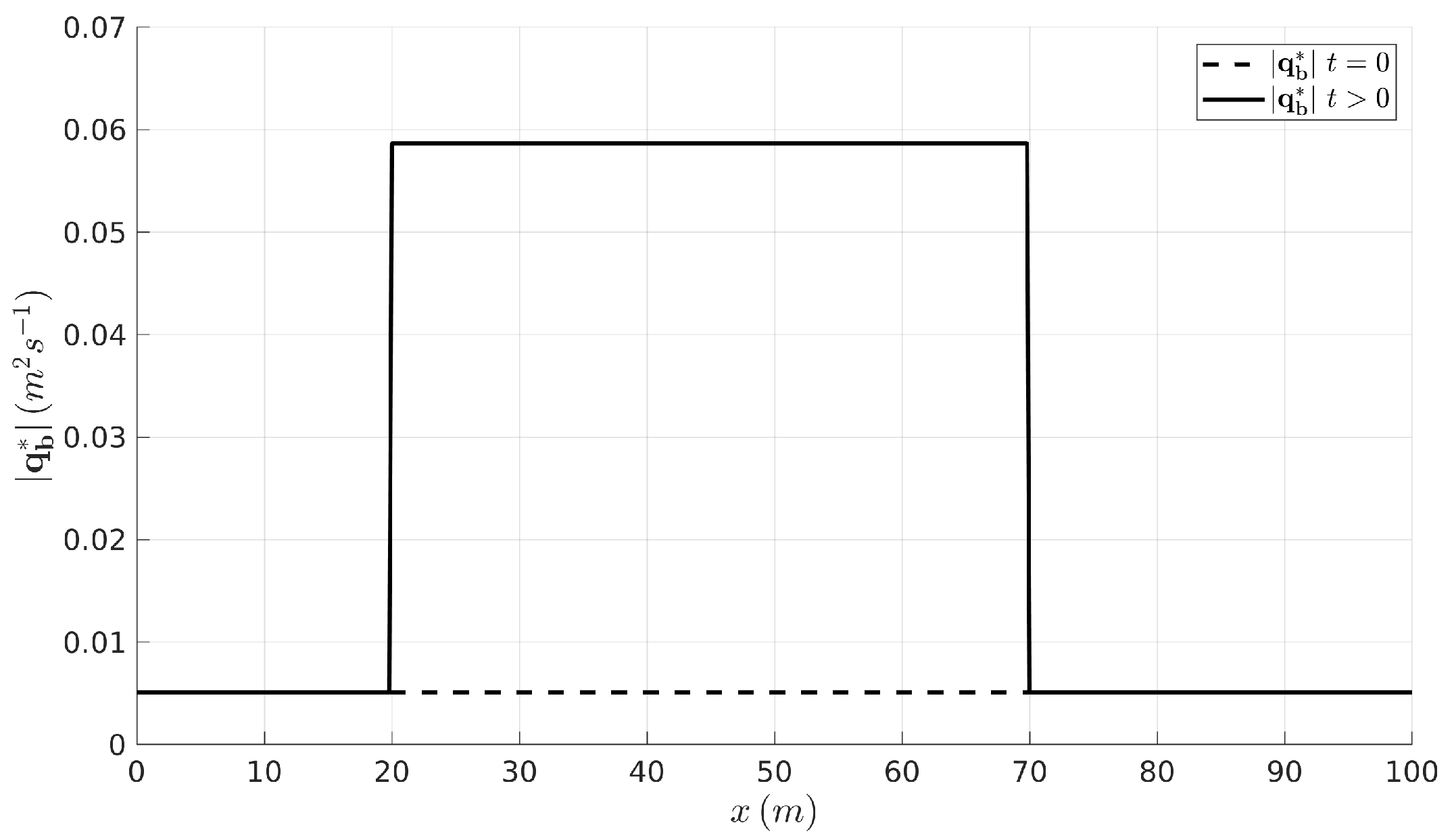
with kg/m, , mm, , and the MPM relation (see Table 1). Using (15)–(16), these local flow features lead to a uniform bedload discharge at the initial time s and a stepped capacity transport rate for any s, as depicted in Figure 2.
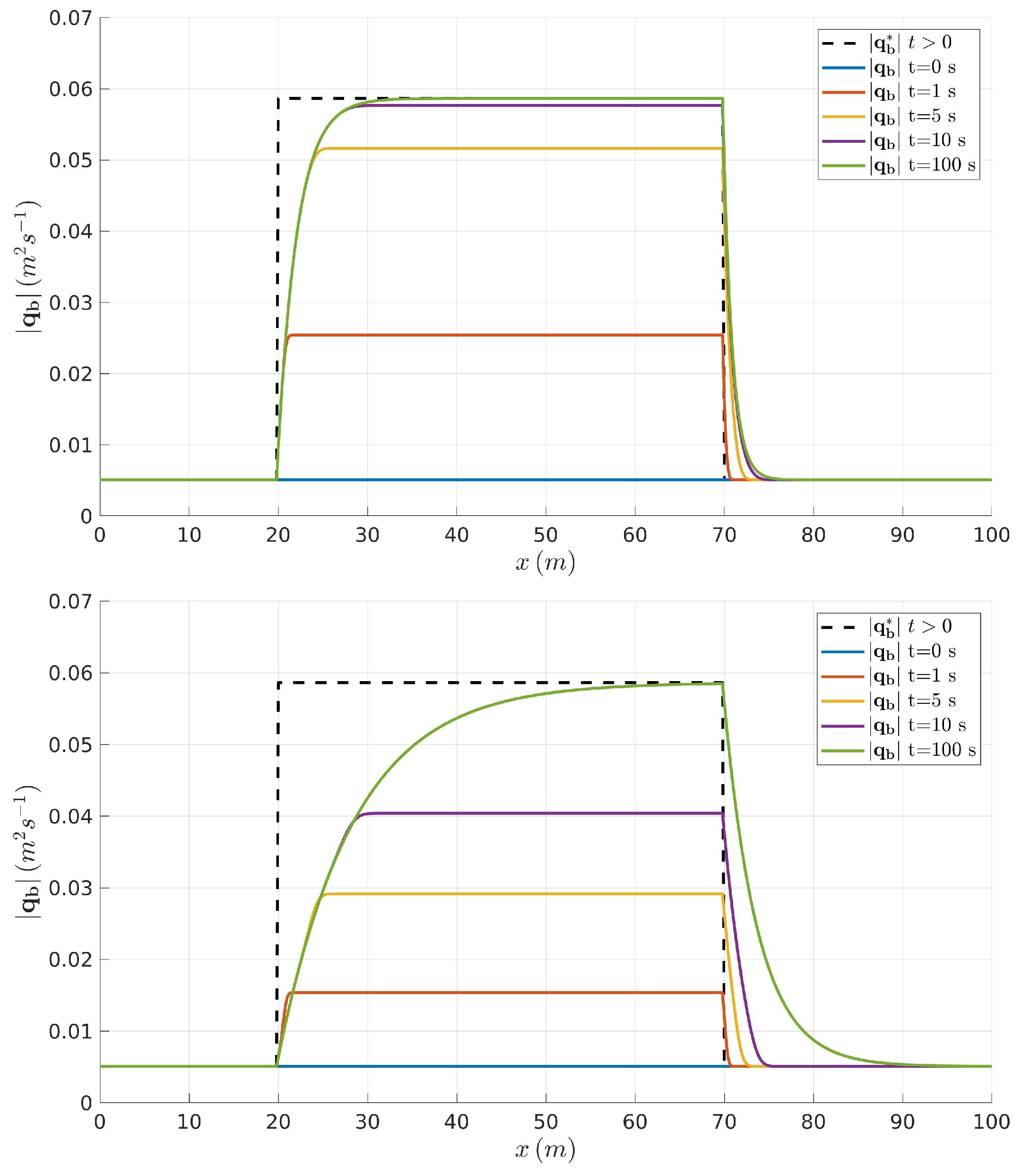
The generalised non-equilibrium model introduces a temporal and spatial delay of the actual transport rate with respect to the capacity value. Figure 3 shows the temporal evolution of the bedload rate in the spatial domain computed using the non-equilibrium model (15)–(17), with (top) and (bottom) . As time increases, the actual solid rate adapts progressively to the capacity rate. Nevertheless, sudden spatial changes of the local flow features, as occurs at m and m, need a length for the actual transport rate to adapt to the transport capacity value even with . Comparing the adaptation of the beload rate to the flow carry capacity with (top) and (bottom) , it is worth noting that the temporal and spatial delay of the non-equilibrium solid discharge respect to the corresponding equilibrium state increases as the entrainment constant decreases.
Furthermore, the net exchange flux through the static-moving bed layers interface can be expressed as (22). Previous non-equilibrium (non-capacity) bedload models [12,20,35,36] assumed a spatial length for the adaptation of the actual bedload solid rate to its equilibrium state and estimate the net exchange vertical flux as
where is a constant parameter which needs to be calibrated for each case. Comparison of method (27) to determine the entrainment/deposition flux with the method proposed in this work () demonstrates that the current model leads to a dynamic adaptation length which depends on the local flow features and scales following
According to (28), higher boundary Shields stresses are associated longer distances for the adaptation of the actual bedload discharge to its equilibrium state (see Figure 3). Contrarily, the lower the entrainment parameter , the larger the dynamic adaptation length. Therefore, high Shields stresses and low entrainment factors enhance non-equilibrium bedload transport states, i.e., highly erosive flow features lead to larger adaptation lengths. Instead, most of the previous models assume a global constant value based on the dominant bed form [36].
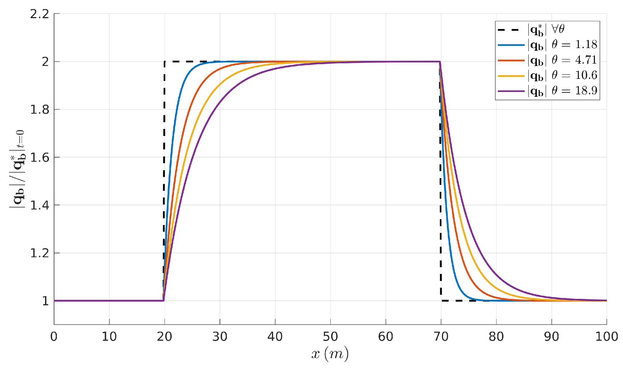
To analyse the influence of the Shields stress on the dynamic adaptation of actual non-equilibrium bedload rate to the equilibrium state, we use the above case but setting a entrainment constant and increasing flow discharges ms. For s the flow is uniform, with m along the whole spatial domain regardless of the discharge, whereas for s a steady step in the flow features is set between 20 m 70 m so that regardless of the flow discharge. The shear stress at the bed surface, hence the Shields stress , increases progressively with the flow discharge as respectively. Figure 4 shows the non-equilibrium bedload rate for s, normalised by the initial uniform equilibrium value , along the whole spatial domain. As the Shields stress at the bed surface increases, the adaptation length increases and enhances the non-capacity state in the bedload transport.
4.2. Dike Breaking by Overtopping Flow Erosion
This experimental test case was carried out by Tingsanchali and Chinnarasri [3] in a 35 m long 1 m wide straight rectangular cross-section flume. In the middle of the flume, a trapezoidal dyke was constructed with a non-cohesive sand of medium diameter mm, solid particle density kg/m and associated bulk porosity . The dyke height over the flume floor was m and the crest width was m, whereas the upward slope and downward slope depends on the laboratory case. The initial water surface elevation was m over the flume floor upstream the dyke. During each experimental case, a constant inlet discharge was set at the flume upstream section. In the original work [3], the temporal evolution of the flow discharge at the dyke crest section and the upstream reservoir level were reported during the whole experiment. Temporal bed elevation data were also provided at probes cm, cm and cm downstream the upward vertex of the dyke crest.
For this case, simulations have been performed using a single-row mesh of 3500 rectangular cells with m and m. The Manning’s roughness coefficient used has been for the flume floor and for the sediment material. The CFL = was set for a full simulated period of 140 s. The Smart formula (Table 1) has been used to compute the bedload transport rate whereas the collapse mechanism has been neglected in this case. Two different benchmarking experiments, C1 and C2, have been used to study the capabilities of both the equilibrium and the non-equilibrium approaches (see Table 2).
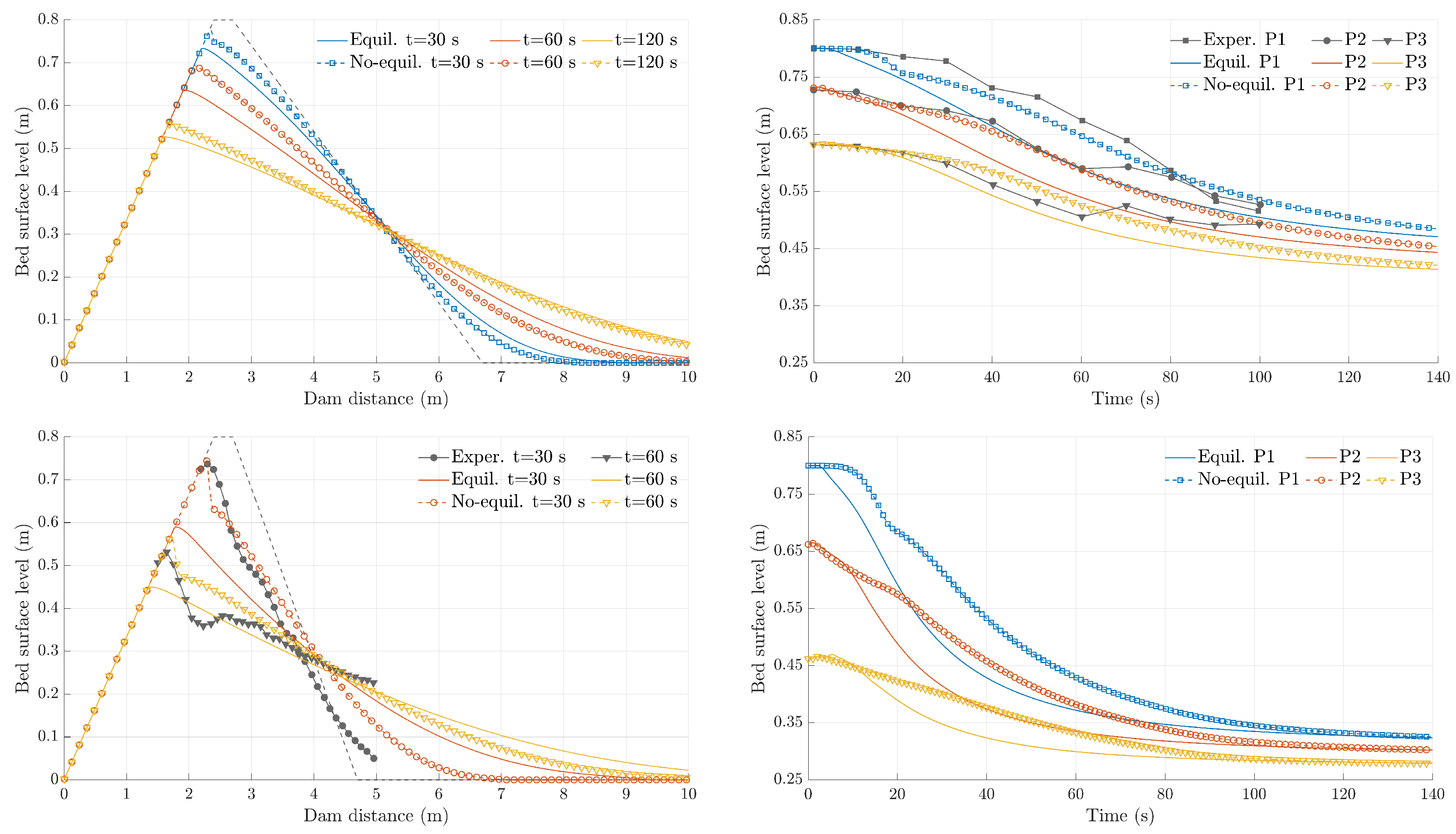
The left column in Figure 5 shows the computed dam profile evolution for both benchmarking tests C1 and C2, considering the equilibrium and non-equilibrium bedload transport assumption, whereas the right column depicts the temporal evolution of the dam level at probes P1, P2 and P3. The black lines show the available experimental data for each test. Analysing the results obtained in both cases C1 and C2, the assumption of non-equilibrium bedload transport leads to a delay on the erosive process in the dam region and hence the change on the bed level is reduced for early stages after the flow starts. However, as the dam erosion progresses, the non-equilibrium bedload transport tends to approach to the equilibrium state and the dam profile level predicted by the non-equilibrium model converges to that obtained by the equilibrium model. It is worth noting that, in case C2, a marked scouring is observed in the experiments just downstream of the dam crest at time s. This scouring was caused likely by 3D behaviour of the flow at the upstream region of the eroded dam. The proposed depth-averaged bedload model is not able to capture the appearance and development of this feature in the bed profile, regardless of the equilibrium or the non-equilibrium approach is selected, due to its 3D nature.
Table 3 shows the Root Mean Square Error (RMSE) of the computed results with both the equilibrium and non-equilibrium models respect to the measured bed level evolution at P1, P2 and P3 in case C1 (available experimental data). Also, for case C2, the RMSE of the computed bed profiles at times s and s respect to the dam profiles measured in the laboratory for the same times are shown in Table 3. Generally, the computed dam level changes with the non-equilibrium approach show a much better agreement with the measured data than those obtained assuming the equilibrium restriction.
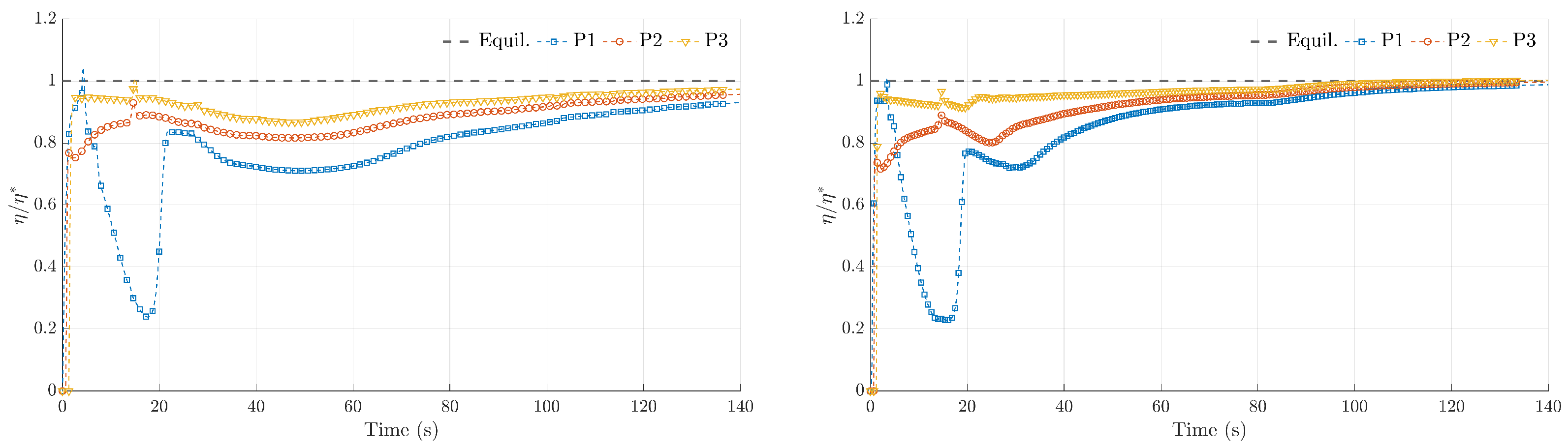
In order to get insight into the non-equilibrium bedload behaviour, the temporal evolution of the thickness of the transport layer at probes P1, P2 and P3, normalised by the corresponding equilibrium value computed from the instantaneous local hydrodynamic features using (8), is depicted in Figure 6 for cases C1 and C2. During the early stages after the overtopping flow starts, non-equilibrium states in the bedload transport layer occur all along the downward dam slope. The closer the dyke crest, the more enhanced is the non-equilibrium state of bedload transport and hence the normalised value generally shows lower values at P1 location than that at probes P2 and P3 during the first flow stages. Then, as the dam erosion progresses, the thickness of the transport layer tends progressively to the equilibrium value () all along the dyke downward side.
The temporal evolution of the computed and measured discharge at the dyke crest and the water surface level at the the upstream reservoir have been plotted in Figure 7 for cases C1 and case C2. Also the Root Mean Square Error (RMSE) of the computed data with respect to the available measured data have been reported in Table 4 considering both equilibrium and non-equilibrium approaches. Considering non-equilibrium conditions for the bedload transport improves clearly the general agreement between the computed and measured evolution of the crest discharge and reservoir level in both benchmarking cases.
4.3. Breach Opening in Homogeneous Dam
This benchmark case aims to explore qualitatively the differences on the numerical modelling of the dambreach opening process using both bedload equilibrium and non-equilibrium approaches. Here we consider one of the experimental dambreach tests carried out at the Laboratório Nacional de Engenharia Civil (LNEC), Lisbon, Portugal, as part of the 6th Workshop on River and Sedimentation Hydrodynamics and Morphodynamics (Online, 24–26 November 2021), supported by Experimental Methods and Instrumentation Committee of the IAHR. The main results obtained during this laboratory campaign are unpublished yet. The experimental data available for this work were provided to the numerical modellers during the first blind stage and hence they are limited. Figure 8 shows a 3D sketch of the initial experimental setup. A homogeneous trapezoidal dam was constructed at the end of a 6 m length m width rectangular cross-section channel. The dam was m height, 1V:2H upward slope, 1V:2.5H downward slope, m base length and m crest width. Downstream the dam, there exists a settling basin, where the elevation of the free surface is zero relatively to the bottom of the upstream reservoir (dam base).
The dam was composed of a non-cohesive silty sand with 25% of fines, solid density 2650 kg/m, median diameter mm, relative compaction of 90% of the Standard Proctor reference value, 10% optimal water content for compaction. At the centerline of the dam crest, a triangular cross-section notch with 1V:1H side slopes and cm deep (see Figure 8) was carved to guide the dambreach process during the early flow stages. Initially, the water level at the upstream reservoir was equal to the height of the model dam ( m) and the free surface at the downstream basin is at the dam toe elevation. Note that the water at the downstream basin is spilt if the elevation is higher than the dam toe. Once the flow started at the notch region and the breach opening process began, the water level at the upstream reservoir was maintained approximately constant by changing the upstream inlet discharge. The maximum inlet discharge allowed in the upstream reservoir is m/s. The test was conducted until the maximum discharge at the upstream reservoir was attained. During the test, the temporal evolution of the inlet discharge at the upstream reservoir was recorded using an electromagnetic flowmeter whereas the water level was obtained from an acoustic probe following the free-surface.
This test has been simulated using an unstructured mesh of almost 16,500 triangular cells, with 50 cm of base cell area and a progressively refined region at the dam and notch zones of cm minimum cell area. At the inlet section of the upstream reservoir, the time series of inlet discharge recorded in the experiment has been imposed during the simulation, whereas free outflow has been allowed at the outlet section at the downstream basin. The Manning’s roughness coefficient has been used for the sediment material in the Manning-Strickler relation . The porosity of the dam layer has been estimated as from the bulk weight of the compacted dam material (90% of the Standard Proctor) and the entrainment and deposition constants have been set to and respectively. The Smart formula (Table 1) has been used to compute the bedload transport rate with the critical Shields stress for the incipient motion . The morphological mechanism plays a key role in this case to model the breach opening due to the collapse of the lateral sides. Based on experimental qualitative observations, a collapse bed slope angle has been set (see Section 3.2). CFL = for a full simulated period of 4500 s.
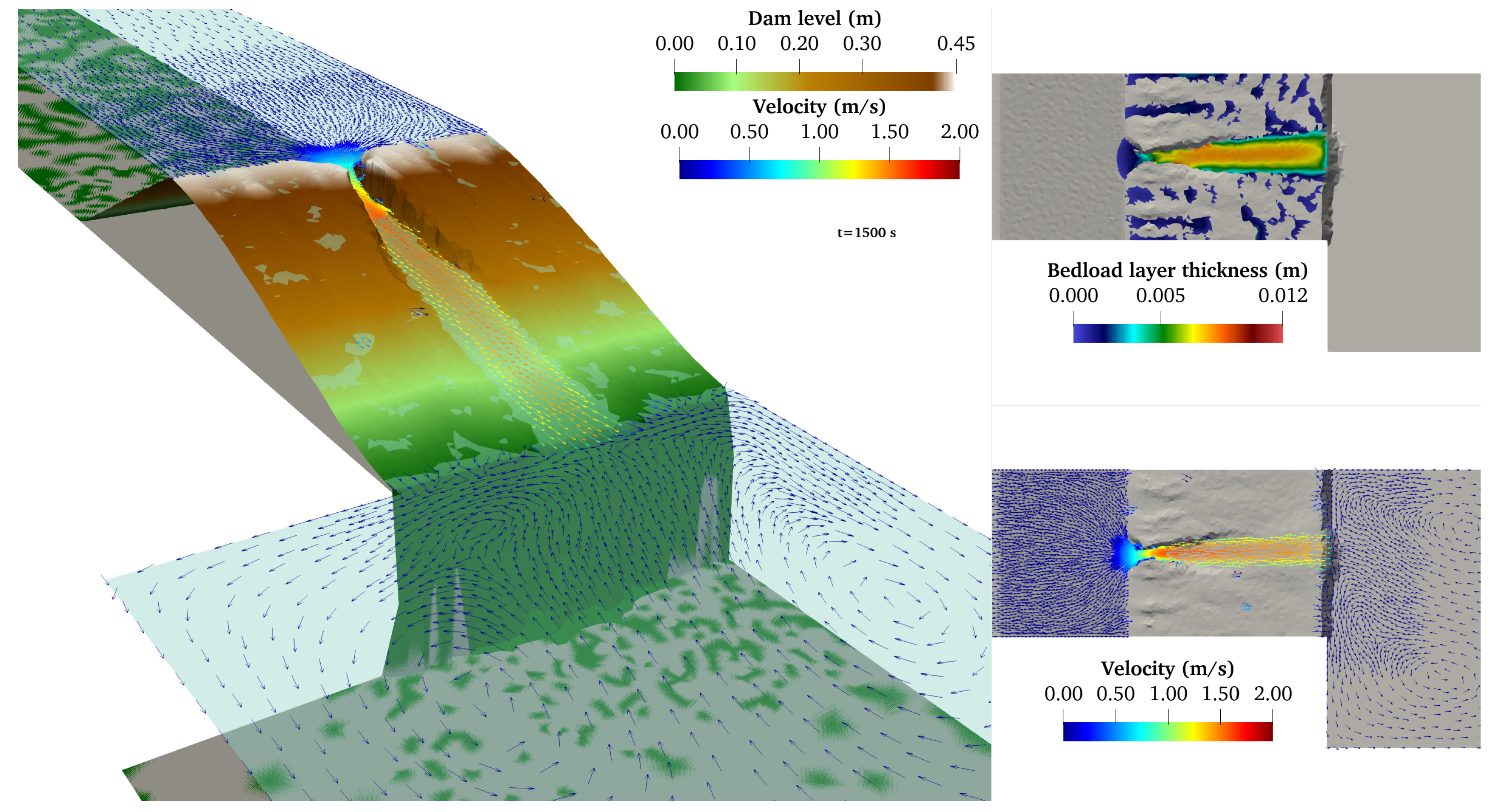
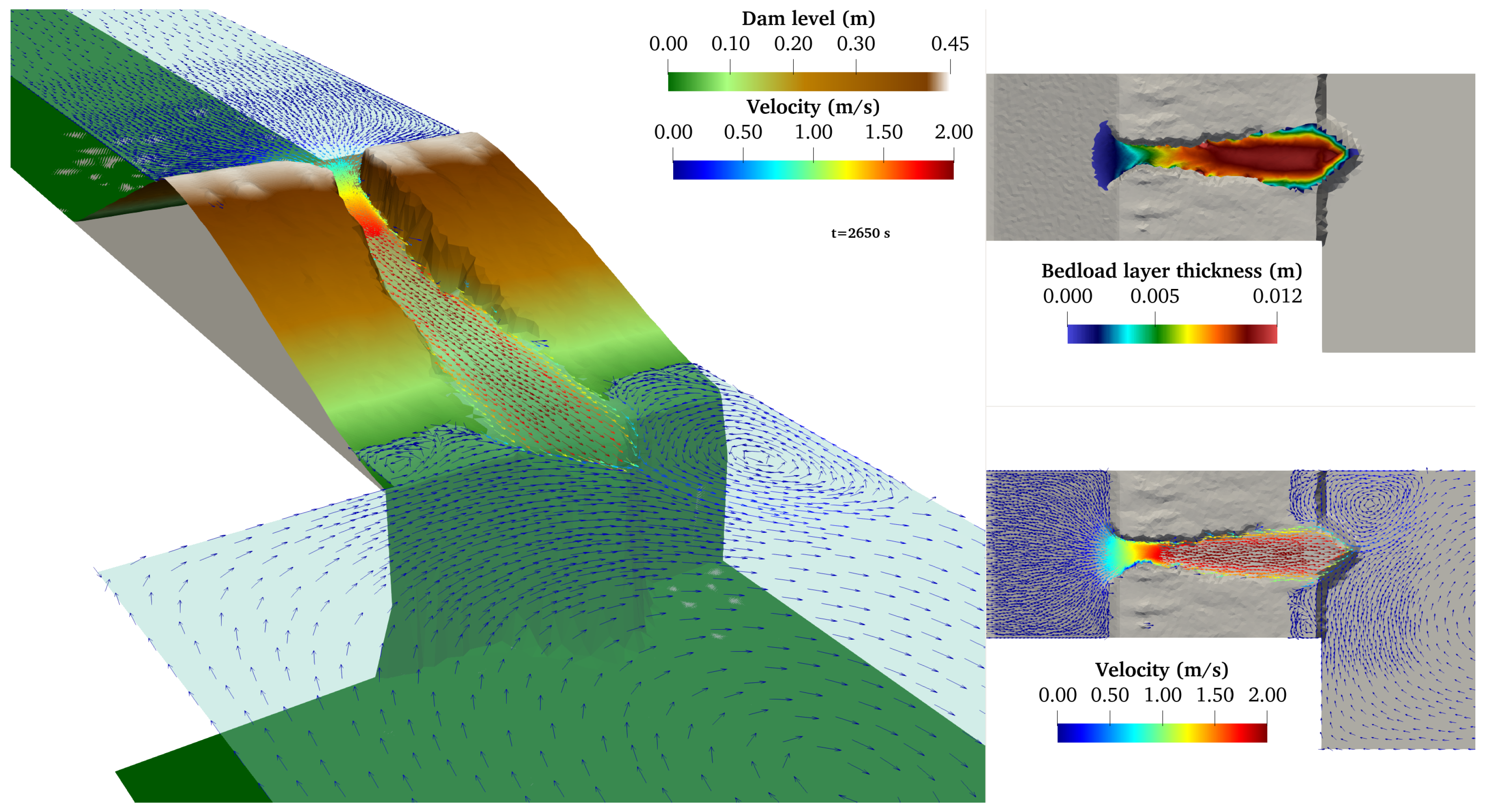
Figure 9, Figure 10, Figure 11 and Figure 12 show a 3D view of the dam topography and free water surface computed with the non-equilibrium model at s, s, s and s respectively. Also the thickness of the bedload transport layer and the flow velocity field at the breach region are shown. The breach opens progressively, increasing its cross-wise width due to the side wall collapse thanks to the collapse mechanism. A couple of coherent vortices appear downstream the dam, as the flow through the breach goes into the downward basin. The thickness of the transport layer increases progressively along the breach, allowing that the mobilized material incorporated to the flow from the breach sides can be transported downstream and reaches the settling basin.
Differences appears in the breach opening process depending on the equilibrium or non-equilibrium approaches selected. Figure 13 depicts (left) the total breach discharge and (right) the upstream reservoir level during the test computed with both equilibrium and non-equilibrium models. The total water discharge at the breach crest cross-section is almost similar using both approaches. Nevertheless, as the breach opens, the reservoir level decreases more markedly with the equilibrium assumption than that using the non-equilibrium model. Note that the experimental test was carried out maintaining an almost-constant water level at the upstream reservoir (solid black line in Figure 13 right). Therefore, the non-equilibrium model seems to approximate better the breach opening process than the equilibrium approach.
Finally, the left column of Figure 14 shows cross-section wetted-area at the dam crest section whereas the right column depicts the averaged flow velocity at the same section. Assuming non-equilibrium bedload transport leads to a slower flow velocity during the early stages of the breach opening and a higher wetted area along the breach region. This hydrodynamic combination reduces the erosive capability of the flow at this region and delays the breach opening process.
5. Conclusions
In this work, a recently developed 2D generalized bedload transport model [30], able to account for equilibrium and non-equilibrium transport conditions, is applied to study the dam breach and dyke erosion processes. This generalized model is based on the grain-scale analysis of the net exchange flux through the static-moving bed layers interface and provide new expressions for the erosion and deposition rates and , respectively. The proposed bedload transport model is supported by a generalized Grass-type formula for the non-equilibrium 2D bedload rate as a function of the transport layer thickness , which must be solved depending on equilibrium or non-equilibrium approach is considered. The 2D morpho-dynamical system of flow-bed conservation equations is solved using and fully-coupled augmented Roe solver [34] whereas the bedload transport layer equation is solved using an upwind scheme. Furthermore, the maximum bed slope is limited using an efficient non-iterative morphological collapse mechanism, which imposes geometrical restrictions on each cell edge.
The proposed model has been benchmarked against dyke erosion and dambreach opening laboratory experiments, involving highly unsteady flows. The non-equilibrium model is able to predict the measured data in all the cases tested, improving the results obtained with the classical equilibrium approach. Furthermore, the effects of the entrainment and deposition constants, and respectively, have also been analysed. When non-equilibrium model is applied, the adaptation of the actual bedload solid rate to the flow carry capacity becomes non-instantaneous and the appearance of bed changes is delayed in time and space. The temporal and spatial delay of the non-equilibrium bedload rate respect to the corresponding flow carry capacity increases as the entrainment constant decreases. Moreover, as the local Shield stress exerted by the flow in the bedload transport layer grows, the equivalent dynamic adaptation length is increased and hence the non-equilibrium states are promoted (see Section 4.1).
In general, considering the unsteady dambreach flow configuration, better predictions of the breach opening mechanism can be obtained using the non-equilibrium approach for the bedload transport rate with moderate values of the exchange entrainment and deposition parameters respect those obtained using the equilibrium model. Numerical results seems to support that considering non-equilibrium conditions for the bedload transport improves the general agreement between the computed results and measured data for overtopping dyke erosion and dambreach opening cases, delaying the breach opening process. However, the non-equilibrium approach requires a careful calibration of the exchange parameters in regions with complex transient processes.
Author Contributions
Conceptualization, S.M.-A. and P.G.-N.; methodology, S.M.-A.; software, S.M.-A. and J.F.-P.; validation, S.M.-A.; resources, P.G.-N.; data curation, S.M.-A.; writing and original draft preparation, S.M.-A.; review and editing, J.F.-P. and P.G.-N.; supervision, P.G.-N.; funding acquisition, S.M.-A. and P.G.-N. All authors have read and agreed to the published version of the manuscript.
Funding
This work has been carried out under the project JIUZ2022-IAR-03: High Performance Computing Tools for Smart Agriculture and Forestry, funded by the University of Zaragoza. This work has been partially funded by the Aragón Government (DGA) through the Fondo Europeo de Desarrollo Regional (FEDER).
Institutional Review Board Statement
Not applicable.
Informed Consent Statement
Not applicable.
Data Availability Statement
Not applicable.
Acknowledgments
Thanks are due to Rui M.L. Ferreira (Instituto Superior Técnico, Universidade de Lisboa, Lisbon, Portugal) for the invitation to participate in the 6th Workshop on River and Sedimentation Hydrodynamics and Morphodynamics (Online, 24–26 November 2021). The resulting experimental data provided for validation of these numerical models is gratefully appreciated.
Conflicts of Interest
The authors declare no conflict of interest.
Abbreviations
The following abbreviations are used in this manuscript:
| FV | Finite Volume |
| RMSE | Root Mean Square Error |
References
- Yang, C. Sediment Transport: Theory and Practice; McGraw-Hill Inc.: New York, NY, USA, 1996. [Google Scholar]
- Juez, C.; Murillo, J.; Garcia-Navarro, P. Numerical assessment of bed-load discharge formulations for transient flow in 1D and 2D situations. J. Hydroinform. 2013, 15, 1234–1257. [Google Scholar] [CrossRef]
- Tingsanchali, T.; Chinnarasri, C. Numerical modelling of dam failure due to flow overtopping. Hydrol. Sci. J. 2001, 46, 113–130. [Google Scholar] [CrossRef]
- Cao, Z.; Day, R.; Egashira, S. Coupled and Decoupled Numerical Modeling of Flow and Morphological Evolution in Alluvial Rivers. J. Hydraul. Eng. 2002, 128, 306–321. [Google Scholar] [CrossRef]
- Hudson, J.; Sweby, P.K. Formulations for Numerically Approximating Hyperbolic Systems Governing Sediment Transport. J. Sci. Comput. 2003, 19, 225–252. [Google Scholar] [CrossRef]
- Goutière, L.; Soares-Frazão, S.; Savary, C.; Laraichi, T.; Zech, Y. One-Dimensional Model for Transient Flows Involving Bed-Load Sediment Transport and Changes in Flow Regimes. J. Hydraul. Eng. 2008, 134, 726–735. [Google Scholar] [CrossRef]
- Castro-Díaz, M.; Fernández-Nieto, E.; Ferreiro, A. Sediment transport models in Shallow Water equations and numerical approach by high order finite volume methods. Comput. Fluids 2008, 37, 299–316. [Google Scholar] [CrossRef]
- Murillo, J.; García-Navarro, P. Weak solutions for partial differential equations with source terms: Application to the shallow water equations. J. Comput. Phys. 2010, 229, 4327–4368. [Google Scholar] [CrossRef]
- Juez, C.; Murillo, J.; García-Navarro, P. A 2D weakly-coupled and efficient numerical model for transient shallow flow and movable bed. Adv. Water Resour. 2014, 71, 93–109. [Google Scholar] [CrossRef]
- Martínez-Aranda, S.; Murillo, J.; García-Navarro, P. A 1D numerical model for the simulation of unsteady and highly erosive flows in rivers. Comput. Fluids 2019, 181, 8–34. [Google Scholar] [CrossRef]
- Wu, W.; Wang, S. One-Dimensional Modeling of Dam-Break Flow over Movable Beds. J. Hydraul. Eng. 2007, 133, 48–58. [Google Scholar] [CrossRef]
- El Kadi Abderrezzak, K.; Paquier, A. One-dimensional numerical modeling of sediment transport and bed deformation in open channels. Water Resour. Res. 2009, 45. [Google Scholar] [CrossRef]
- Cao, Z.; Li, Z.; Pender, G.; Hu, P. Non-capacity or capacity model for fluvial sediment transport. Proc. Inst. Civil Eng. Water Manag. 2012, 165, 193–211. [Google Scholar] [CrossRef]
- Fernández-Nieto, E.; Lucas, C.; Morales-de Luna, T.; Cordier, S. On the influence of the thickness of the sediment moving layer in the definition of the bedload transport formula in Exner systems. Comput. Fluids 2014, 91, 87–106. [Google Scholar] [CrossRef]
- Bohorquez, P.; Ancey, C. Particle diffusion in non-equilibrium bedload transport simulations. Appl. Math. Model. 2016, 40, 7474–7492. [Google Scholar] [CrossRef]
- Van-Rijn, L. Principles of Sediment Transport in Rivers, Estuaries and Coastal Seas; Aqua Publications: Amsterdam, The Netherlands, 1993; Chapter 10, Bed Material Transport, Erosion and Deposition in Non-Steady and Non-Uniform Flow. [Google Scholar]
- Cao, Z.; Hu, P.; Pender, G. Multiple Time Scales of Fluvial Processes with Bed Load Sediment and Implications for Mathematical Modeling. J. Hydraul. Eng. 2011, 137, 267–276. [Google Scholar] [CrossRef]
- El Kadi Abderrezzak, K.; Paquier, A.; Gay, B. One-dimensional numerical modelling of dam-break waves over movable beds: Application to experimental and field cases. Environ. Fluid Mech. 2008, 8, 169–198. [Google Scholar] [CrossRef]
- Zhang, S.; Duan, J. 1D finite volume model of unsteady flow over mobile bed. J. Hydrol. 2011, 405, 57–68. [Google Scholar] [CrossRef]
- Soliman, M.R.; Ushijima, S. Equilibrium and Non-equilibrium Sediment Transport Modeling Based On Parallel MACS Algorithm. J. Jpn. Soc. Civil Eng. 2013, 69, 79–86. [Google Scholar] [CrossRef]
- van Rijn, L. Sediment Transport, Part I: Bed Load Transport. J. Hydraul. Eng. 1984, 110, 1431–1456. [Google Scholar] [CrossRef]
- Lee, H.; Hsu, I. Investigation of Saltating Particle Motions. J. Hydraul. Eng. 1994, 120, 831–845. [Google Scholar] [CrossRef]
- Ferreira, R.M.L.; Franca, M.J.; Leal, J.G.A.B.; Cardoso, A.H. Mathematical modelling of shallow flows: Closure models drawn from grain-scale mechanics of sediment transport and flow hydrodynamics. Can. J. Civil Eng. 2009, 36, 1605–1621. [Google Scholar] [CrossRef]
- Charru, F. Selection of the ripple length on a granular bed sheared by a liquid flow. Phys. Fluids 2006, 18, 121508. [Google Scholar] [CrossRef]
- Zech, Y.; Soares-Frazão, S.; Spinewine, B.; Grelle, N.L. Dam-break induced sediment movement: Experimental approaches and numerical modelling. J. Hydraul. Res. 2008, 46, 176–190. [Google Scholar] [CrossRef]
- Fernández-Nieto, E.D.; Luna, T.M.d.; Narbona-Reina, G.; Zabsonré, J.d.D. Formal deduction of the Saint-Venant-Exner model including arbitrarily sloping sediment beds and associated energy. Math. Model. Numer. Anal. 2017, 51, 115–145. [Google Scholar] [CrossRef]
- Singh, U.; Ahmad, Z. Transport rate and bed profile computations for clay–silt–gravel mixture. Environ. Earth Sci. 2019, 78, 432. [Google Scholar] [CrossRef]
- Singh, U.K.; Jamei, M.; Karbasi, M.; Malik, A.; Pandey, M. Application of a modern multi-level ensemble approach for the estimation of critical shear stress in cohesive sediment mixture. J. Hydrol. 2022, 607, 127549. [Google Scholar] [CrossRef]
- Martínez-Aranda, S.; Murillo, J.; García-Navarro, P. A comparative analysis of capacity and non-capacity formulations for the simulation of unsteady flows over finite-depth erodible beds. Adv. Water Resour. 2019. in print. [Google Scholar] [CrossRef]
- Martínez-Aranda, S.; Meurice, R.; Soares-Frazão, S.; García-Navarro, P. Comparative analysis of HLLC- and Roe-based Models for the simulation of a dam-break flow in an erodible channel with a 90º bend. Water 2021, 13, 1840. [Google Scholar] [CrossRef]
- Grass, A. Sediments Transport by Waves and Currents; Department of Civil Engineering, University College: London, UK, 1981. [Google Scholar]
- Murillo, J.; García-Navarro, P. An Exner-based coupled model for two-dimensional transient flow over erodible bed. J. Comput. Phys. 2010, 229, 8704–8732. [Google Scholar] [CrossRef]
- Godlewski, E.; Raviart, P.A. Numerical Approximation of Hyperbolic Systems of Conservation Laws; Springer: New York, NY, USA, 1996. [Google Scholar]
- Martínez-Aranda, S.; Murillo, J.; García-Navarro, P. Comparison of new efficient 2D models for the simulation of bedload transport using the augmented Roe approach. Adv. Water Resour. 2021, 153, 103931. [Google Scholar] [CrossRef]
- Wu, W.; Vieira, D.; Wang, S. One-Dimensional Numerical Model for Nonuniform Sediment Transport under Unsteady Flows in Channel Networks. J. Hydraul. Eng. 2004, 130, 914–923. [Google Scholar] [CrossRef]
- Wu, W. Computational River Dynamics; CRC Press: London, UK, 2007. [Google Scholar]
Figure 1.
Sketch of the generalized bedload transport model at grain-scale.

Figure 2.
Bedload transport rate evolution for classical equilibrium formulations.

Figure 3.
Bedload transport rate evolution for the generalised non-equilibrium model with (top) and (bottom) .
Figure 3.
Bedload transport rate evolution for the generalised non-equilibrium model with (top) and (bottom) .

Figure 4.
Normalised bedload transport rate for the generalised non-equilibrium model with increasing Shields stresses .
Figure 4.
Normalised bedload transport rate for the generalised non-equilibrium model with increasing Shields stresses .

Figure 5.
Dam profile evolution for (top row) case C1 and (bottom row) case C2 with equilibrium and non-equilibrium approaches: (left) dam profile at different times and (right) bed level evolution at P1, P2 and P3.
Figure 5.
Dam profile evolution for (top row) case C1 and (bottom row) case C2 with equilibrium and non-equilibrium approaches: (left) dam profile at different times and (right) bed level evolution at P1, P2 and P3.

Figure 6.
Temporal evolution of the transport layer thickness at P1, P2 and P3: (left) case C1 and (right) case C2.
Figure 6.
Temporal evolution of the transport layer thickness at P1, P2 and P3: (left) case C1 and (right) case C2.

Figure 7.
Computed and measured temporal evolution of (left column) the discharge at the dyke crest and (right column) the upstream reservoir water surface level: (top row) case C1 and (bottom row) case C2.
Figure 7.
Computed and measured temporal evolution of (left column) the discharge at the dyke crest and (right column) the upstream reservoir water surface level: (top row) case C1 and (bottom row) case C2.

Figure 8.
3D sketch of the experimental setup (initial condition) at the Laboratório Nacional de Engenharia Civil (LNEC, Lisbon). Detail of the initial triangular notch at the dam crest.
Figure 8.
3D sketch of the experimental setup (initial condition) at the Laboratório Nacional de Engenharia Civil (LNEC, Lisbon). Detail of the initial triangular notch at the dam crest.

Figure 9.
Dambreach opening at s with non-equilibrium model: (left) 3D view of the dam level and water surface; (right top) thickness of the bedload transport layer and (right bottom) depth-averaged velocity field.
Figure 9.
Dambreach opening at s with non-equilibrium model: (left) 3D view of the dam level and water surface; (right top) thickness of the bedload transport layer and (right bottom) depth-averaged velocity field.

Figure 10.
Dambreach opening at s with non-equilibrium model: (left) 3D view of the dam level and water surface; (right top) thickness of the bedload transport layer and (right bottom) depth-averaged velocity field.
Figure 10.
Dambreach opening at s with non-equilibrium model: (left) 3D view of the dam level and water surface; (right top) thickness of the bedload transport layer and (right bottom) depth-averaged velocity field.

Figure 11.
Dambreach opening at s with non-equilibrium model: (left) 3D view of the dam level and water surface; (right top) thickness of the bedload transport layer and (right bottom) depth-averaged velocity field.
Figure 11.
Dambreach opening at s with non-equilibrium model: (left) 3D view of the dam level and water surface; (right top) thickness of the bedload transport layer and (right bottom) depth-averaged velocity field.

Figure 12.
Dambreach opening at s with non-equilibrium model: (left) 3D view of the dam level and water surface; (right top) thickness of the bedload transport layer and (right bottom) depth-averaged velocity field.
Figure 12.
Dambreach opening at s with non-equilibrium model: (left) 3D view of the dam level and water surface; (right top) thickness of the bedload transport layer and (right bottom) depth-averaged velocity field.

Figure 13.
Dambreach evolution with equilibrium and non-equilibrium approaches: (left) dam discharge and (right) upstream reservoir level.
Figure 13.
Dambreach evolution with equilibrium and non-equilibrium approaches: (left) dam discharge and (right) upstream reservoir level.

Figure 14.
Dambreach evolution with equilibrium and non-equilibrium approaches: (left) cross-section wetted-area of the breach and (right) averaged flow velocity at the dam crest section.
Figure 14.
Dambreach evolution with equilibrium and non-equilibrium approaches: (left) cross-section wetted-area of the breach and (right) averaged flow velocity at the dam crest section.


Table 1.
Grass-type interaction factor G for transport rate formulations.
| Formulation | ||||
|---|---|---|---|---|
| MPM | 0.047 | |||
| Nielsen | 0.047 | |||
| Fernandez-Luque | 0.037 | |||
| Wong | 0.0495 | |||
| Smart | 0.047 | |||
| Wu | 0.030 |
In the Smart formula, the parameter accounts for the bed slope along the bedload transport direction.
Table 2.
Setup for benchmarking cases C1 and C2.
| Case | (L/s) | ||||
|---|---|---|---|---|---|
| C1 | 1V:3H | 1V:5H | 1.05 | 0.24 | 0.012 |
| C2 | 1V:3H | 1V:3H | 1.23 | 0.34 | 0.017 |
Table 3.
RMSE for dam level evolution data in benchmarking cases C1 and C2.
| Data Series | Equil. | No-Equil. |
|---|---|---|
| C1—Bed level in P1 | 0.057 m | 0.023 m |
| C1—Bed level in P2 | 0.053 m | 0.022 m |
| C1—Bed level in P3 | 0.033 m | 0.020 m |
| C2—Bed level profile at s | 0.112 m | 0.061 m |
| C2—Bed level profile at s | 0.029 m | 0.039 m |
Table 4.
RMSE for the crest discharge and reservoir level data in benchmarking cases C1 and C2.
| Data Series | Equil. | No-Equil. |
|---|---|---|
| C1—Dam discharge | 10.94 L/s | 3.10 L/s |
| C1—Reservoir level | 0.055 m | 0.019 m |
| C2—Dam discharge | 45.02 L/s | 11.76 L/s |
| C2—Reservoir level | 0.116 m | 0.034 m |
Disclaimer/Publisher’s Note: The statements, opinions and data contained in all publications are solely those of the individual author(s) and contributor(s) and not of MDPI and/or the editor(s). MDPI and/or the editor(s) disclaim responsibility for any injury to people or property resulting from any ideas, methods, instructions or products referred to in the content. |
© 2023 by the authors. Licensee MDPI, Basel, Switzerland. This article is an open access article distributed under the terms and conditions of the Creative Commons Attribution (CC BY) license (https://creativecommons.org/licenses/by/4.0/).
Share and Cite
MDPI and ACS Style
Martínez-Aranda, S.; Fernández-Pato, J.; García-Navarro, P. Non-Equilibrium Bedload Transport Model Applied to Erosive Overtopping Dambreach. Water 2023, 15, 3094. https://0-doi-org.brum.beds.ac.uk/10.3390/w15173094
AMA Style
Martínez-Aranda S, Fernández-Pato J, García-Navarro P. Non-Equilibrium Bedload Transport Model Applied to Erosive Overtopping Dambreach. Water. 2023; 15(17):3094. https://0-doi-org.brum.beds.ac.uk/10.3390/w15173094
Chicago/Turabian StyleMartínez-Aranda, Sergio, Javier Fernández-Pato, and Pilar García-Navarro. 2023. "Non-Equilibrium Bedload Transport Model Applied to Erosive Overtopping Dambreach" Water 15, no. 17: 3094. https://0-doi-org.brum.beds.ac.uk/10.3390/w15173094
Note that from the first issue of 2016, this journal uses article numbers instead of page numbers. See further details here.