
Sensitivity Analysis of Runoff and Wind with Respect to Yellow River Estuary Salinity Plume Based on FVCOM

1
The Center for Ports and Maritime Safety (CPMS), Dalian Maritime University, Dalian 116026, China
2
Shandong Marine Resource and Environment Research Institute, Yantai 265503, China
3
The Department of Food and Biochemical Engineering, Yantai Vocational Collage, Yantai 264025, China
4
College of Oceanography and Atmosphere, Ocean University of China, Qingdao 266100, China
5
Marine Environmental Monitoring Central Station, State Oceanic Administration, Yantai 264000, China
*
Author to whom correspondence should be addressed.
Water 2023, 15(7), 1378; https://0-doi-org.brum.beds.ac.uk/10.3390/w15071378
Submission received: 19 February 2023
/
Revised: 29 March 2023
/
Accepted: 30 March 2023
/
Published: 3 April 2023
(This article belongs to the Special Issue Impact of Atmospheric and River Inputs on the Transfer of Elements and Organic Matter to the Ocean)
Abstract
:In 2020, Yellow River runoff was more than twice as much as past years, and the proportion of strong winds was also higher than that in past years, which will inevitably lead to a change in salinity plume distribution in the Yellow River Estuary and Laizhou Bay. Based on FVCOM numerical modelling, this paper presents the spatial salinity distribution and dispersion of the Yellow River Estuary and Laizhou Bay during the wet and dry seasons in 2020. We used data from six tidal and current stations and two salinity stations to verify the model, and the results showed that the model can simulate the local hydrodynamic and salinity distribution well. The influence of river discharge and wind speed on salinity diffusion was then investigated. The simulation results showed that under the action of residual currents, fresh water from the Yellow River spread to Laizhou Bay, and the low salinity area of Laizhou Bay was mainly distributed in the northwest. The envelope area of 27 psu isohaline can account for about one-quarter of Laizhou Bay in the wet season, while the low-salinity area was only concentrated near the estuary of Yellow River in the dry season. River discharge mainly affects the diffusion area and depth of fresh water, and wind can change the diffusion structure and direction. In the wet season, with the increase in wind speed, the surface area of the plume decreased gradually, and the direction of the fresh water plume changed counterclockwise from south to north. During the dry season, the plume spread to the northwest along the nearshore. The increase in wind speed in the early stage increased the surface plume area, and the plume area decreased above a wind speed of 10 m/s due to the change in the turbulence structure. The model developed and the results from this study provide valuable information for establishing robust water resource regulations for the Yellow River. This is particularly important to ensure that the areas with low salinity in the Yellow River Estuary will not decrease and affect the reproduction of fish species.
1. Introduction
Low-salinity areas have become important economic development areas for marine fishery, especially around estuaries. The change in salinity around estuaries will have great influence on biological survival, mariculture, and underwater construction. Differing from the ocean area, estuaries fully reflect their own complexity in both offshore marine structure and ecological environment. Tidal circulation and salinity transport processes around estuaries are usually very complex. The situation is further complicated due to the mixing of salt and fresh water and the simultaneous effects of runoff, tides, waves, wind, and offshore currents [1]. When fresh water flows from estuaries into open nearshore waters, a plume diffusion structure is formed near estuaries due to different invasion rates of density currents inside and outside estuaries [2]. Xia [3] performed numerical simulation of the salinity distribution in the mouth of the Fair River in North Carolina, and found that winds with different speeds had different influences on the diffusion of low-salinity water in the estuary through separate and coupled studies of tides, wind, and runoff. The diffusion and distribution of salinity around the estuary were affected by the river discharge [4,5], tide [6,7], and wind [8,9]. Fong and Geyer [10] showed that wind had a very strong effect on the diffusion of low-salinity water offshore, and wind speed and direction can both affect diffusion structure and direction. Cheng and Casulli [11] showed that astronomical tides had an impact on salinity diffusion around estuaries, especially on the vertical distribution of salinity. Wang [12] found that estuary salinity fluctuated with changes in tidal current, tide, wind, and fresh water flow. Estuarine salinity diffusion has a great impact on coastal ecology. Zhou and Matthew [13] found that the Mississippi River’s discharge affected the salinity distribution of the estuaries in the northern Gulf of Mexico, and showed that river discharge, wind, and season were important factors affecting estuarine salinity diffusion. Salmela [14] showed that high river discharge promoted the development of an estuary plume in the Baltic River estuary. Under the action of low river discharge and wind, the Baltic Sea estuary developed counterclockwise circulation, and high river discharge and salinity stratification promoted the development of clockwise circulation. Coogan [15] showed that river discharge was the main factor controlling the seasonal variation of salinity; but in a short time, wind became the main factor. Mixing and dispersion in the nearshore and estuarine area are complicated, and the underlying processes that underpin this complexity are the spatiotemporal varying structure of turbulence [16] and the complex interactions of nearshore currents [17].
The Yellow River (YR) is the main river that flows into the Bohai Sea (BHS). YR runoff significantly decreased under the influence of natural factors, reservoir construction, and other human factors, and serious long-term flow interruption occurred [18]. This will have an effect on the salinity field near the estuary and even the whole BHS. Figure 1 shows the location (a) and the annual YR runoff from 1952 to 2017 (b) observed in Lijin station. The runoff from the YR to the sea changes dynamically. In 1964, the YR runoff reached a maximum of 1.06 × 10⁸ m3. In 2002, the YR runoff reached only 4.19 × 10⁶ m3. After 2002, runoff was regulated and increased [19].
Dramatic changes in the runoff of the YR caused dynamic change in salinity in the BHS, especially in Laizhou Bay (LZB). In the 20th century, the mean salinity of Bohai Bay increased by 2 psu due to the decrease of the YR’s runoff [20]. Lin et al. [21] analyzed the salinity data of the observation stations around the BHS from 1960 to 1997 and found that the surface salinity of BHB increased by 0.074 psu per year. Wang et al. [22] observed and analyzed the salinity changes in the estuarine area before and after the YR runoff regulation event of 2002, indicating that the increased salinity value around the YR Estuary after the runoff regulation was over two times greater than before.
The YR Estuary is a typical continental estuary with frequent evolution [23], and has been a frequent focus of research. Wang [19] used a numerical model to show that the salinity in the YR Estuary had obvious seasonal variations, indicating that the impact of runoff on salinity distribution was huge. Liu [24] simulated and revealed the influence of wind and tide on salinity distribution around the YR Estuary. Shi [25] used the numerical model ROMS to study the influence of runoff into the sea on the salinity distribution of LZB. Based on the numerical model, Cheng [26] studied the changes and differences in salinity diffusion caused by runoff and topographic changes since the YR changed its estuary three times. A series of studies have shown that tide, wind, runoff, and other factors affect the direction and structure of salinity diffusion around estuaries. However, previous studies focused more on long-term changes in salinity, and did not pay much attention to the changes during a particular time. According to the statistics of Lijin station, the YR’s runoff into the sea during the wet season in 2020 was more than two times higher than the average of previous years. This paper analyzed the influence of runoff and wind on salinity plume based on FVCOM
The paper is organized as follows. The first part is the introduction, and the materials and methods are shown in part two. The third part describes the salinity distribution of the areas near the YR Estuary and in LZB during the wet and dry seasons in 2020. The fourth part discusses the influence of different runoff volumes and wind speeds on YR plume diffusion. The final part describes the study’s conclusions.
2. Materials and Method
2.1. FVCOM Model
FVCOM is a 3D nearshore ocean model based on an unstructured triangular grid [27,28], and has a high ability to simulate complex conditions near estuaries. The control equation is similar to POM, including nonlinear advection, free surface, runoff, vertical mixed 2.5 order turbulent closed mode, etc. The vertical σ coordinate system can better fit the complex seabed topography, and the unstructured grid can better fit the complex shoreline. FVCOM discretizes the governing equations, making its computation more efficient and geometric processing more flexible. It has been widely used in the simulation of nearshore and regional ocean areas, and has achieved good results [29,30,31].The governing equations are shown as follows:
- (a)
- momentum equation
- (b)
- continuity equation
- (c)
- salinity equation
2.2. Boundary Conditions
The boundary conditions for the salinity at the surface and bottom are as follows:
where AH is the horizontal heat diffusion coefficient; α is the angle formed from the sea floor; is the precipitation rate; is the evaporation rate; D is the total depth; H is the water depth below the average sea level; σ increases from the seabed (σ = −1) to the sea surface (σ = 0); and is the height of the free sea above the average sea level.
2.3. Model Setting
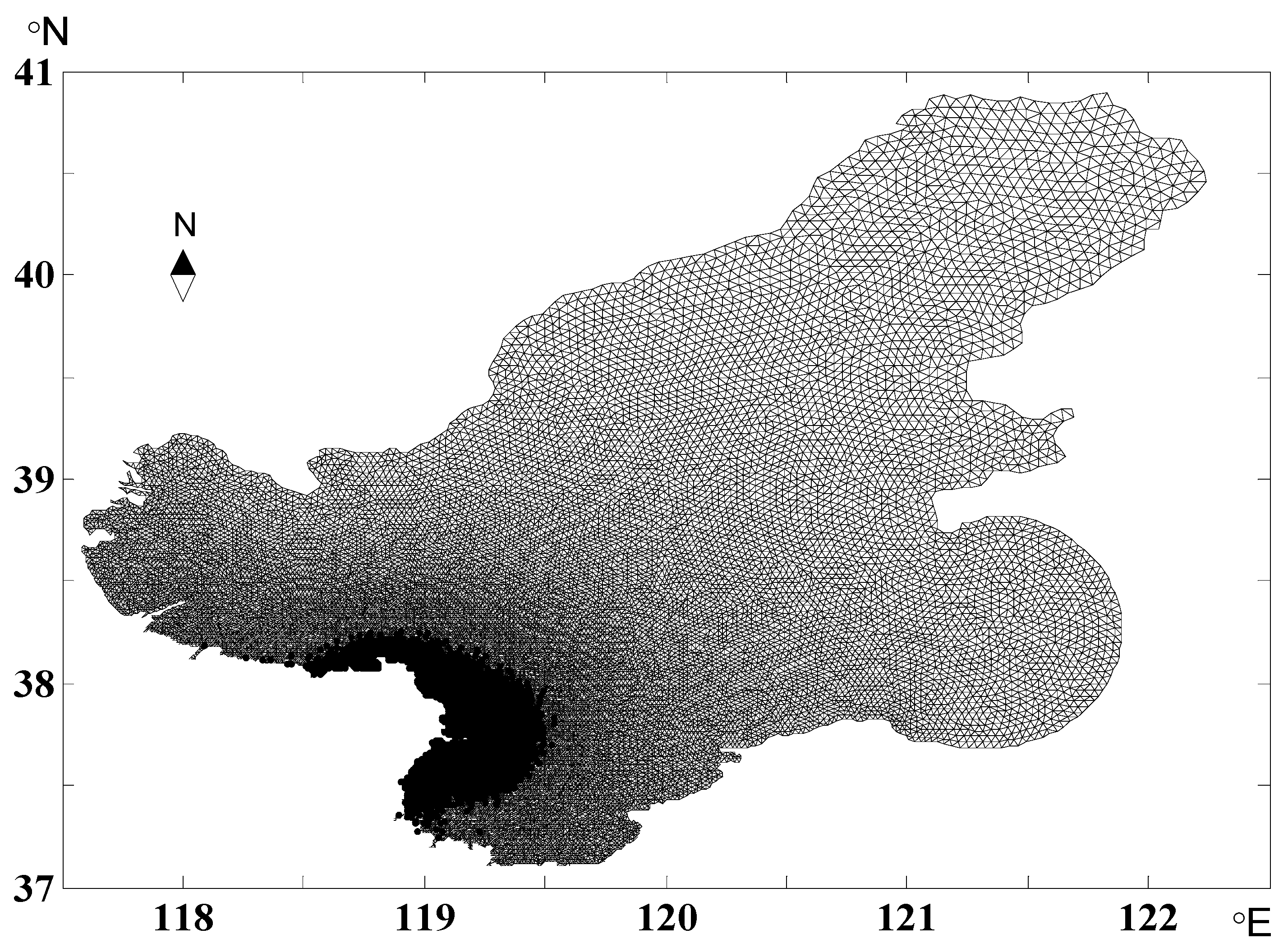
In this paper, the simulated area was the whole BH, and the grid near the YR Estuary was refined. The size of the grid, especially the location of the estuary, has a great influence on fresh water diffusion [32,33]. Therefore, a careful treatment of the refined region is essential to ensure accuracy. According to Chinese standards for liquid diffusion [34] and the width of the estuary, the minimum grid was ~50 m, and there were 100,428 units and 51,499 nodes in total. Figure 2 shows the detailed grid information. The vertical direction was divided into 20 sigma layers. The model adopted a cold start, and the mode calculation adopted an internal and external mode-splitting algorithm, in which the internal mode time step was set to 0.5 s, and the external mode time step was set to 5 s, which could well meet the requirements of calculation accuracy. The salinity diffusion rates in the wet season (July–August) and the dry season (January–February) were simulated respectively. The simulation time of the wet season was from 1 July 2020 to 31 August 2020, and the simulation time of the dry season was from 1 January 2020 to 29 February 2020. The results of February and August were primarily analyzed.
- A.
- River discharge
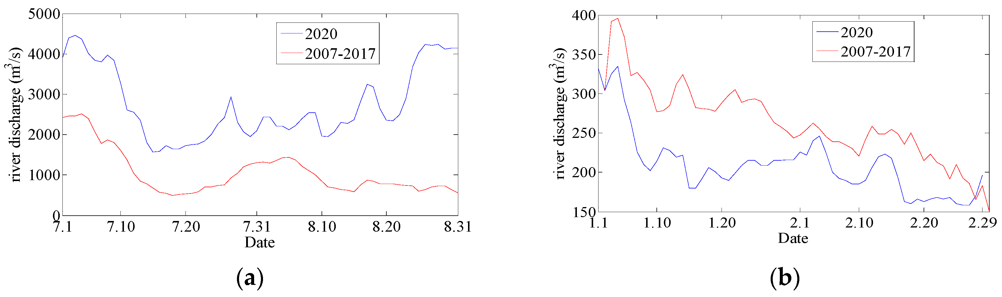
In this model, day-by-day river discharge data were obtained from Lijin Station of YR. Figure 3 shows the variation of the river discharge from the YR into the sea in the wet and dry seasons in 2020. The average river discharge into the sea in 2020 was 2761.935 m3/s in the wet season, and 209.783 m3/s in the dry season. Figure 3 shows the statistical results of multiyear average daily river discharge data during the dry and wet periods from 2007 to 2017. Additionally, the statistical results of multiyear daily average river discharge data in the dry season and wet season from 2007 to 2017 are presented. From 2007 to 2017, the average river discharge in the YR Estuary was 1059.595 m3/s. The average river discharge in the dry season was 264.662 m3/s. Compared to the previous year, the river discharge into the BHS during the dry season changed little in 2020, but the average river discharge during the wet season was 2.6 times higher than the average of the previous years.
- B.
- Wind
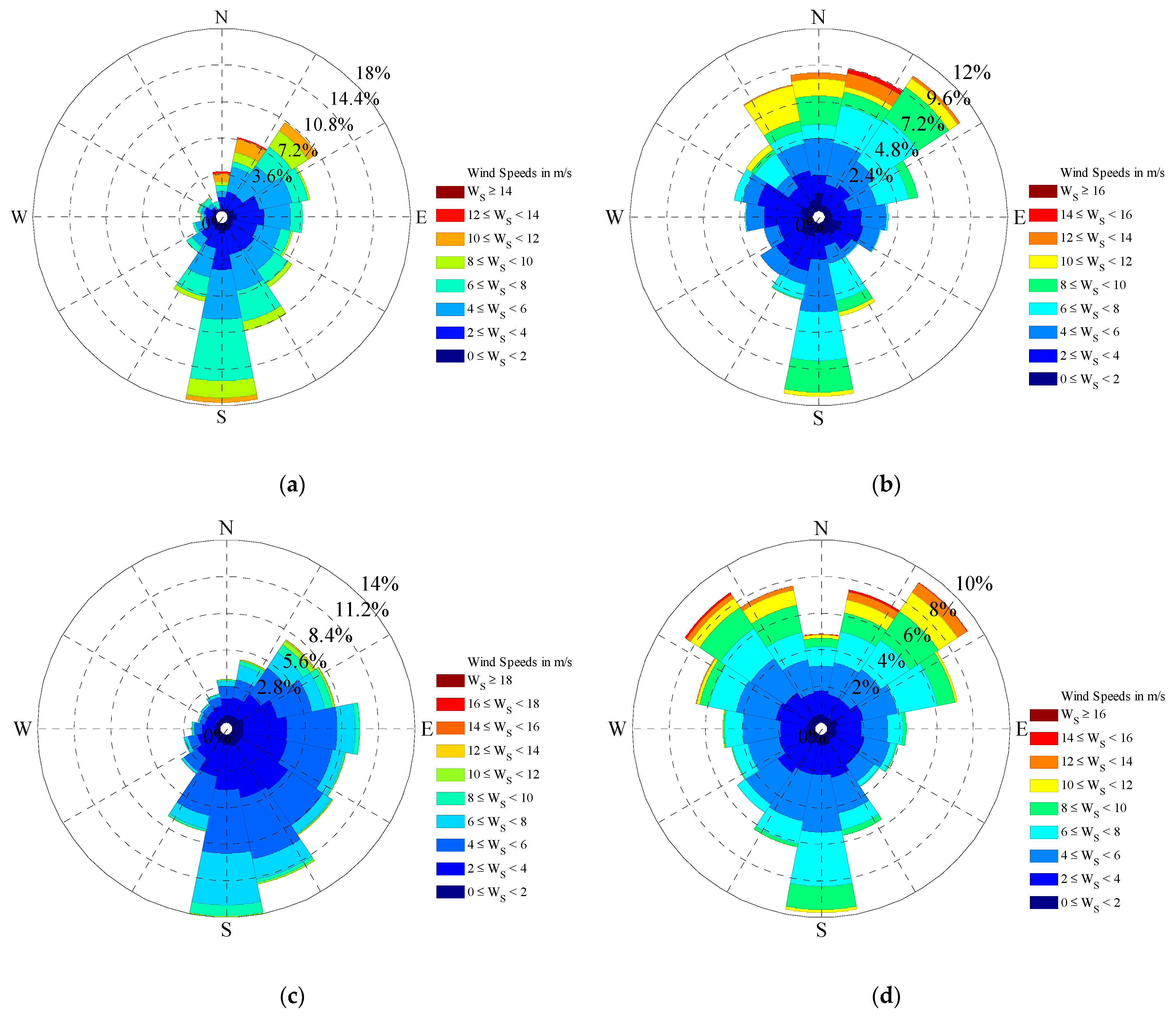
The wind data used for the model were derived from ERA5 (ECMWF Reanalysis V5) with a resolution of 0.25° × 0.25°. Figure 4a,b shows wind roses near the YR Estuary during wet and dry seasons in 2020, and Figure 4c,d shows the wind roses near the YR Estuary during the wet and dry seasons from 2007 to 2017. The main wind direction near the YR Estuary was south in the summer and northeast in the winter. Compared with the statistics from 2007 to 2017, there was a higher proportion of main wind direction and an increased proportion of high wind speed in summer in 2020.
- C.
- Tide
Eight major tidal components (M2, S2, N2, K2, K1, O1, P1, and Q1) were selected for the model, and the open boundary conditions were defined according to harmonic constants.
- D.
- Salinity
The initial salinity field of the model used SODA (Simple Ocean Data Assimilation) data. In the simulation process, the salinity of fresh water was set as 0 psu, and the open boundary salinity was set as 32 psu.
2.4. Model Verification
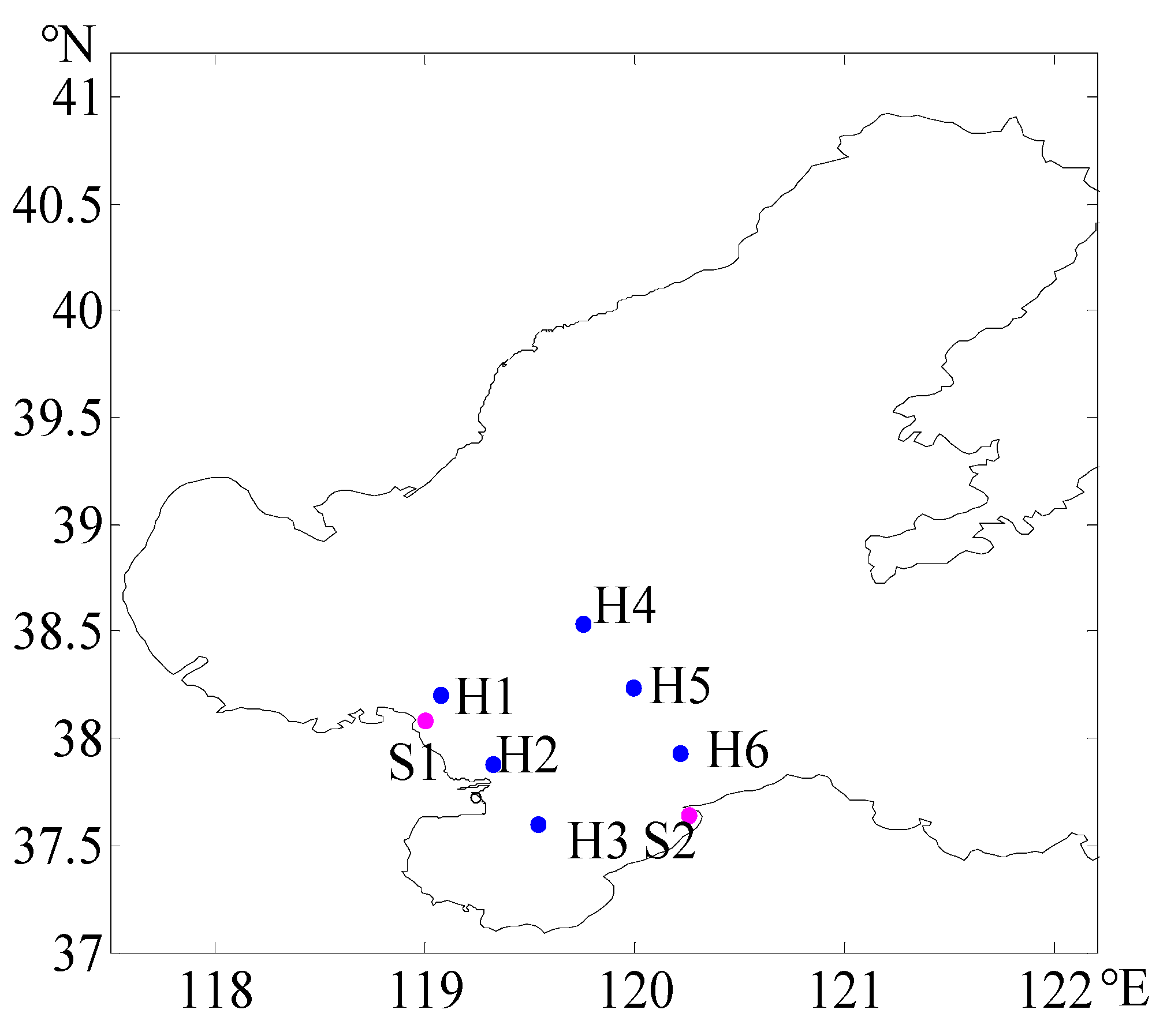
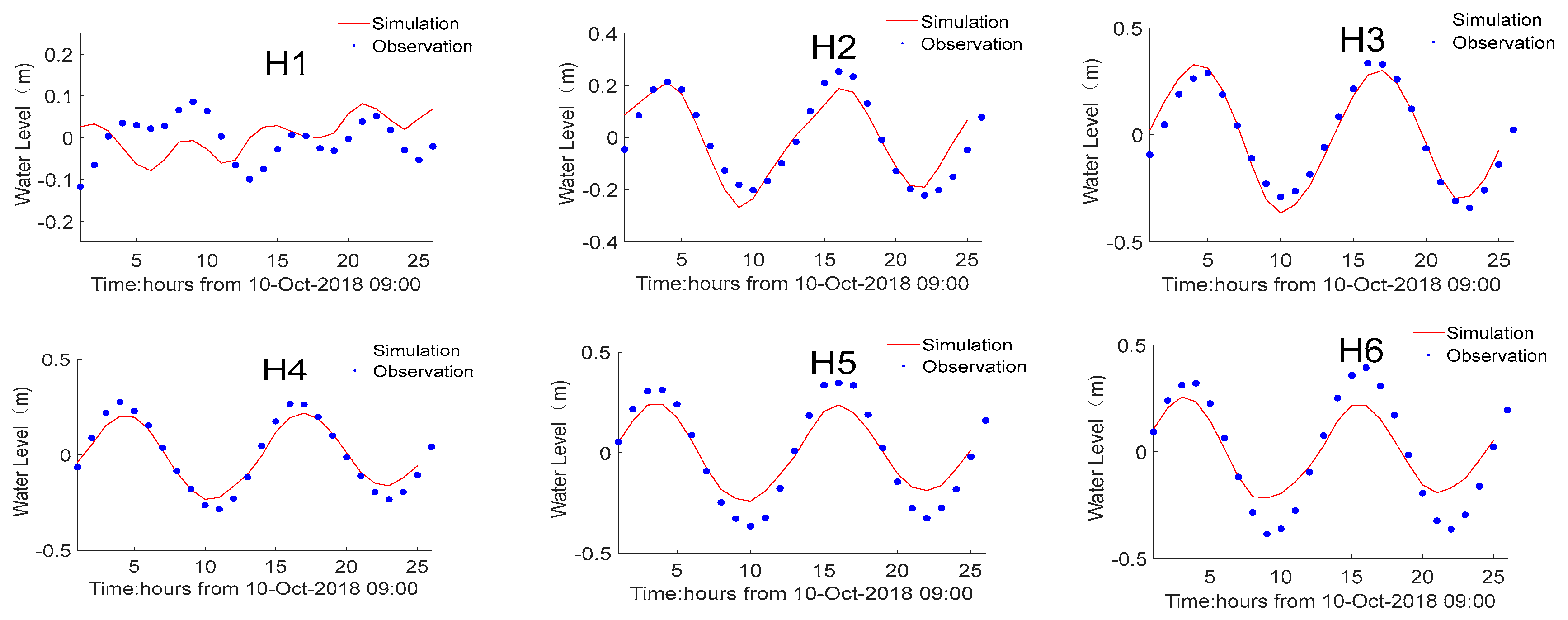
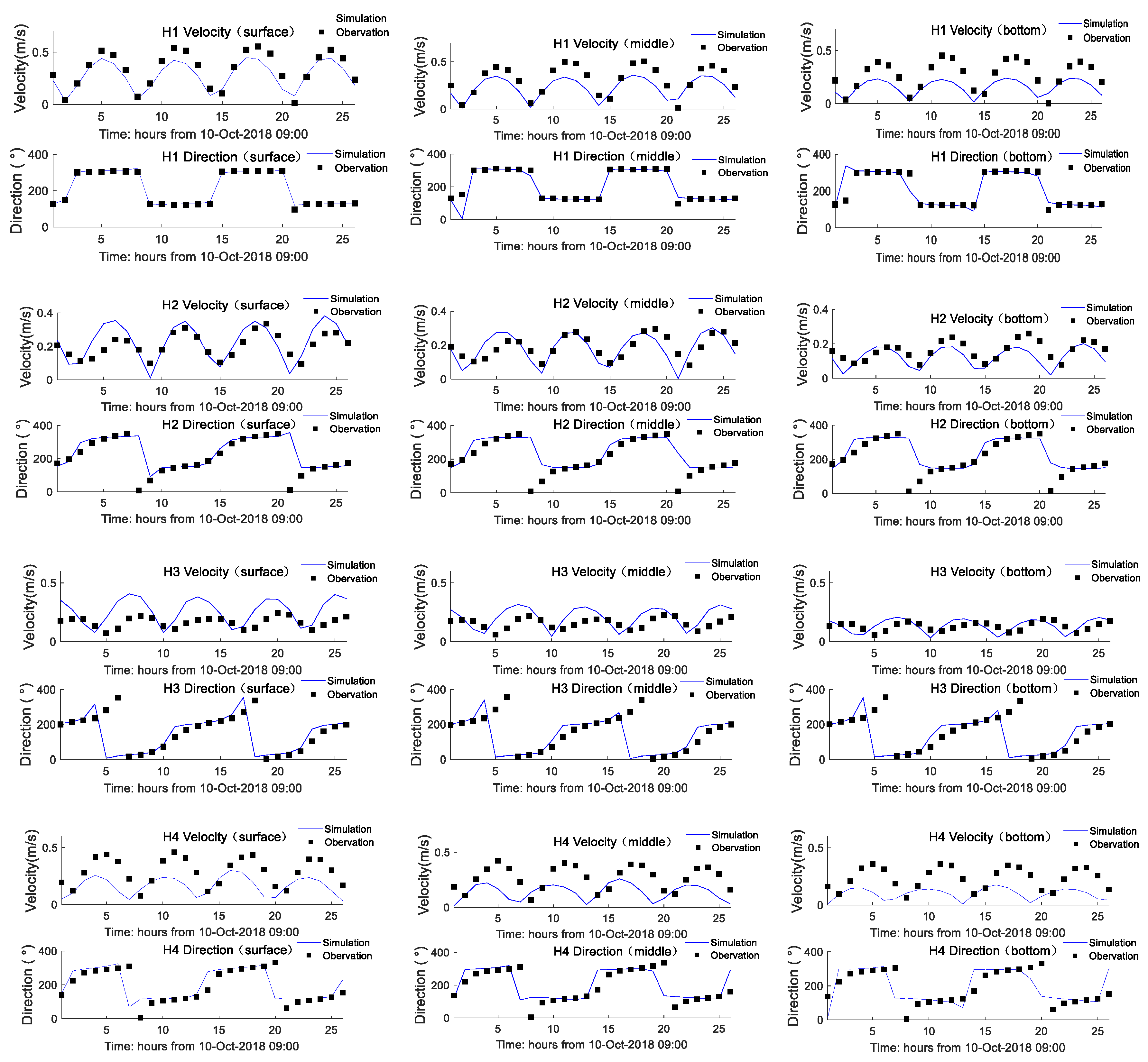
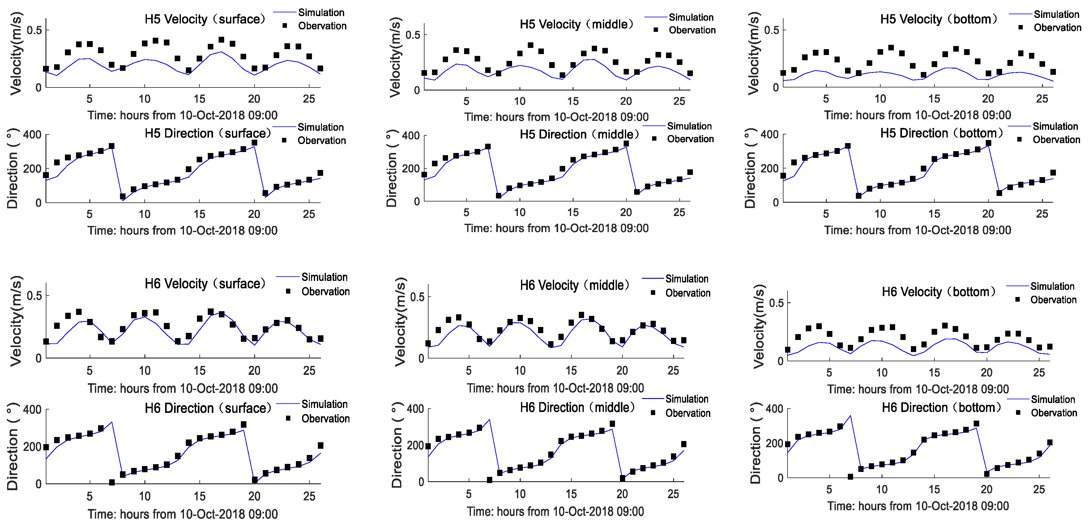
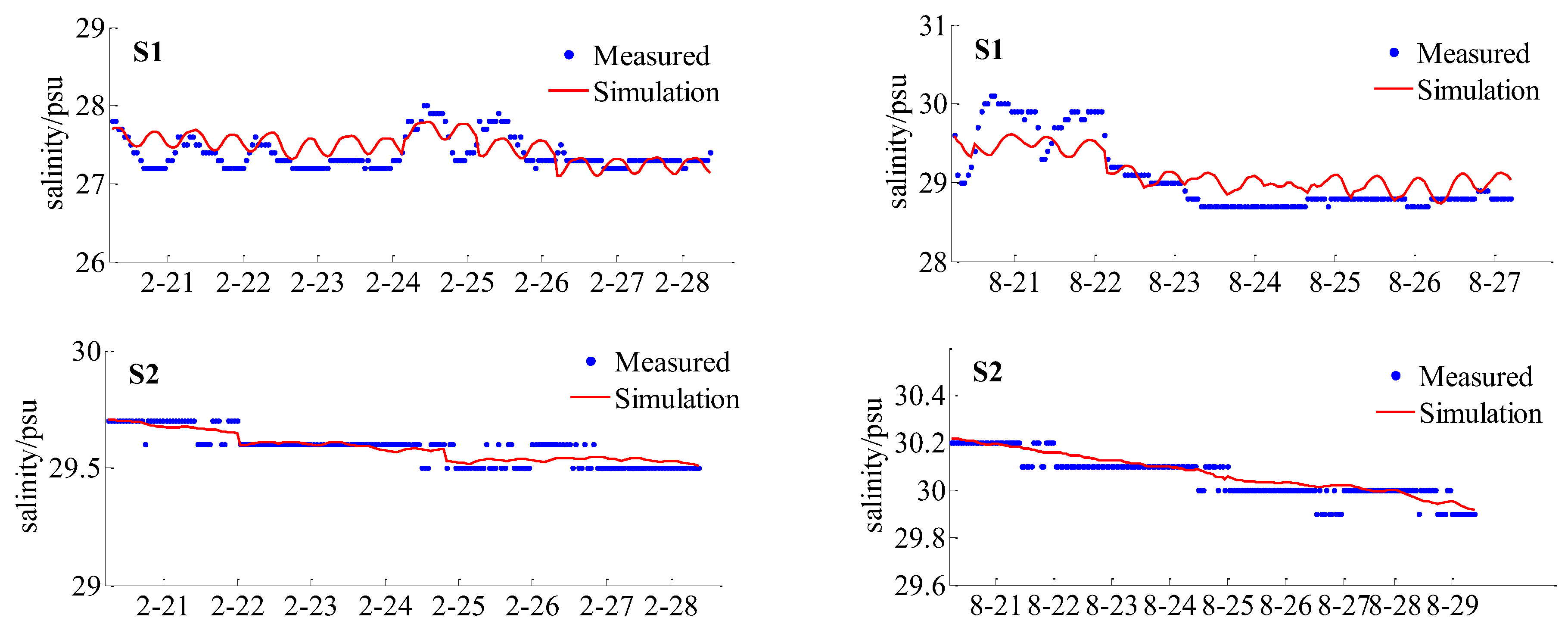
In order to verify the accuracy of the model, we took 6 tidal and current stations and 2 salinity stations for verification. The data on tidal currents and tide levels came from the observations of the research group, the instruments used were JFE and RBR, respectively, and the sampling frequency was 1 h. The salinity data came from the observation data of the Ministry of Natural Resources, the observing instrument was RBR CTD, and the sampling frequency was also 1 h. Figure 5 and Table 1 show the location and the detail of the stations, respectively. Figure 6, Figure 7 and Figure 8 show the verification of tide, current, and salinity, respectively. The correlation coefficient (r) was used to judge the fit of the numerical model (Table 2). The comparison results showed that the calculated salinity value was basically consistent with the measured value. The S1 and H1 stations were close to the YR Estuary, and thus they were greatly affected by the runoff; therefore, the simulation of salinity and water level did not agree with the measure data well (Figure 6). The S2 station was far from the YR Estuary and was less affected by the runoff, and the absolute difference was within 0.1 psu. The calculation results basically reflected the hydrodynamic and salinity changes in research area.
3. Results
3.1. Distribution of Surface Current in the Wet and Dry Seasons
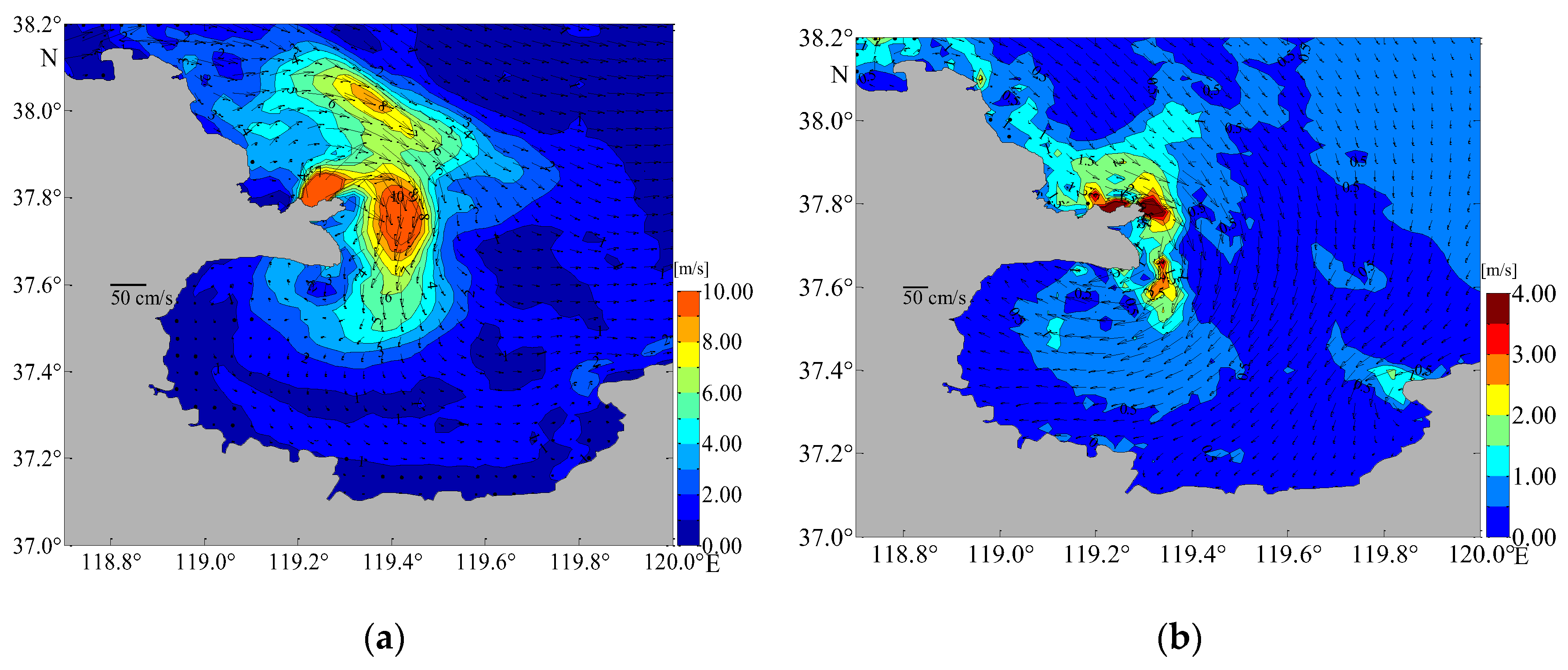
The YR discharge was the main reason for the distribution of salinity in LZB. Under the action of residual currents, fresh water from the YR flowed to LZB. Figure 9 shows the distribution of the residual current field in the wet and dry seasons. The high velocity area is mainly concentrated near the YR Estuary and the southern part of LZB. Under the influence of topography and the Coriolis force, there was a phenomenon that the fresh water from the YR would drift south. Additionally, the direction of the tide was also one of the reasons for the YR plume to spread southward.
3.2. Horizontal Distribution Characteristics of Salinity Fields around the Yellow River Estuary and Laizhou Bay
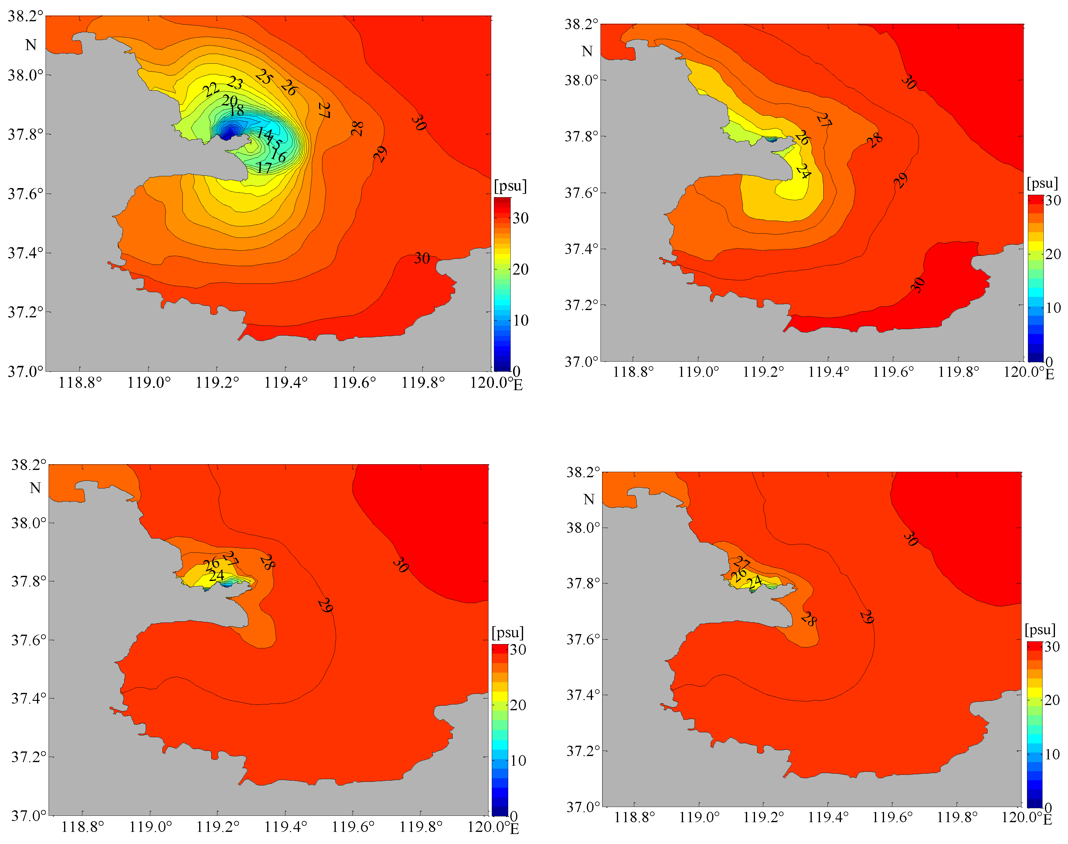
Figure 10 shows the spatial distribution of surface and bottom salinity in the wet and dry seasons. There was an obvious stratification phenomenon near the YR Estuary and LZB in summer, and the salinity distributions between the surface and bottom layer were very different. The vertical distribution of salinity was almost uniform in winter. Due to the influence of river discharge, the salinity distributions in the wet season and the dry season were very different. In the wet season, fresh water from the YR affected nearly the entire LZB. In the dry season, fresh water had an obvious tendency to spread to the middle of LZB. Due to the limitation of river discharge, fresh water from the YR only affected the northwest part of LZB. The isohaline of 27 psu is an important index to measure the salinity distribution. The area near the isohaline of 27 psu is suitable for marine organisms to inhabit and spawn. In the wet season, the salinity front of 27 psu could spread to the middle of LZB, accounting for about one-quarter of the whole LZB. During the dry season, the area below 27 psu salinity was only concentrated near the estuary of the YR.
The research showed that the YR’s fresh water diffused toward LZB in both wet and dry seasons by using the latest data from 2020. In summer, the southeastern wind was dominant near the estuary of the YR, and the diffusion of low-salinity water to the southeast was restricted. Under the action of surface currents, the low-salinity water diffused to LZB. In winter, the northern wind was dominant, and the low-salinity water had an obvious southward diffusion trend, but only a small area of low salinity was formed around the YR Estuary due to the shortage of fresh water.
3.3. Vertical Distribution Characteristics of Salinity in Laizhou Bay
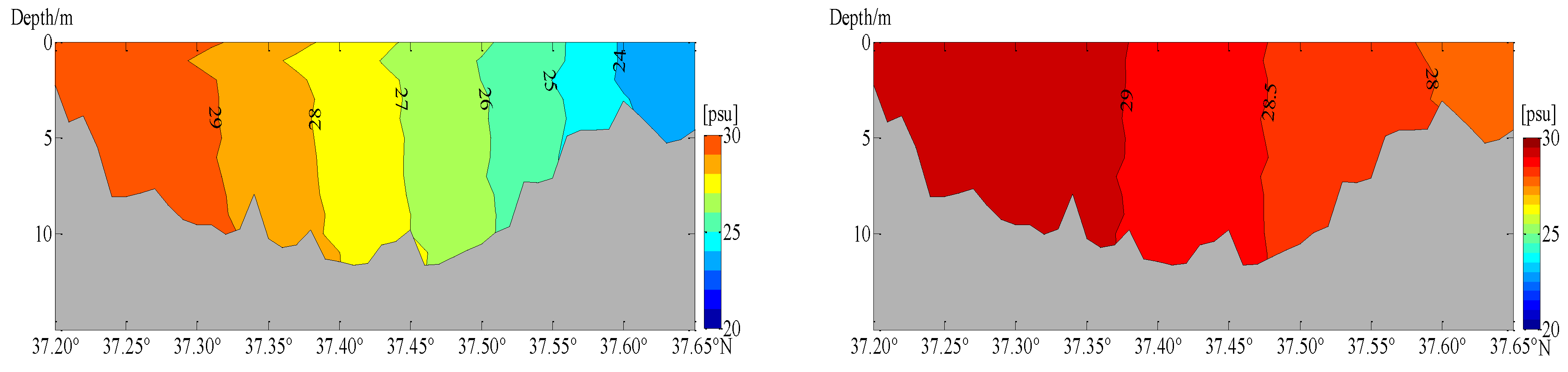
In the salt profile analysis in LZB, we took the location most greatly affected by tide and residual current as an example, and the salinity diffusion phenomenon was analyzed. The section at 119.3° E was selected to study salinity diffusion (Figure 11) in the range of 37.2° N–37.65° N. In the wet season, the river discharge was large and the area affected by YR fresh water in LZB was large. There were many horizontal layers of salinity and the salinity front spreading towards LZB was obvious. During the dry season, the salinity of the whole LZB was high, ranging from 28 to 30 psu. In summer, the salinity exchange at the upper layer was more intense, so the salinity front was more prominent. As it spread to the south of LZB, the surface water with low salinity decreased gradually, causing the salinity mixing zone to become shallower and shallower. In winter, there was very little fresh water and the wind speed was high, causing the vertical distribution of salinity to be relatively uniform.
4. Discussions
The river discharge into the sea from the YR in the wet season in 2020 was 2.6 times higher than the average of previous years. The proportion of high wind speed (≥15 m/s) was also slightly larger than previous years. The particularity of river discharge and wind speed certainly changed the spatial and temporal distribution of salinity near the YR Estuary and LZB in 2020, and continued to affect it in the short term. It was necessary to investigate the influence of river discharge and wind speed. In order to explore the effects of river discharge and wind speed on salinity diffusion near the YR Estuary and LZB, a series of numerical experiments were set up, as shown in Table 3.
4.1. Influence of River Discharge on Salinity Diffusion
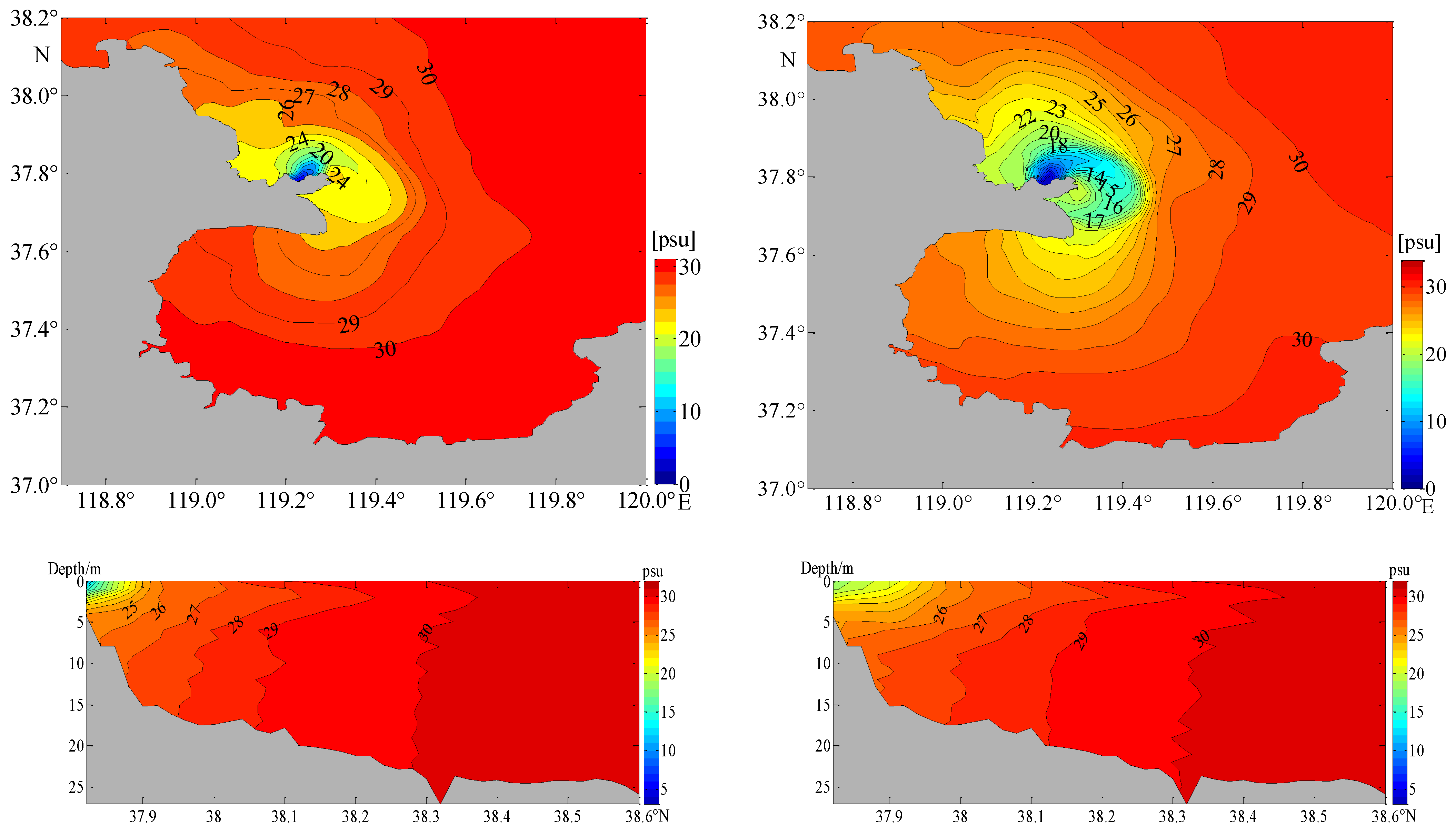
The average river discharge during the wet season in 2020 was 2761.9 m3/s (case 2), and the average river discharge during the wet season from 2007 to 2017 was 1059.6 m3/s (case 1). The volume of river discharge mainly affected the area, distance, and depth of salinity diffusion. Figure 12 (top) shows the surface salinity distribution of the two cases. Figure 12 (bottom) shows the vertical salinity distribution of the two cases. With increasing runoff, the horizontal diffusion area of the plume became larger and the diffusion distance of the salinity front became longer, and the diffusion depth of low salinity water became deeper at the same location. In addition, fresh water from the YR can directly affected the offshore seabed.
4.2. Influence of Different Wind Speeds on Salinity Diffusion in the Wet Season
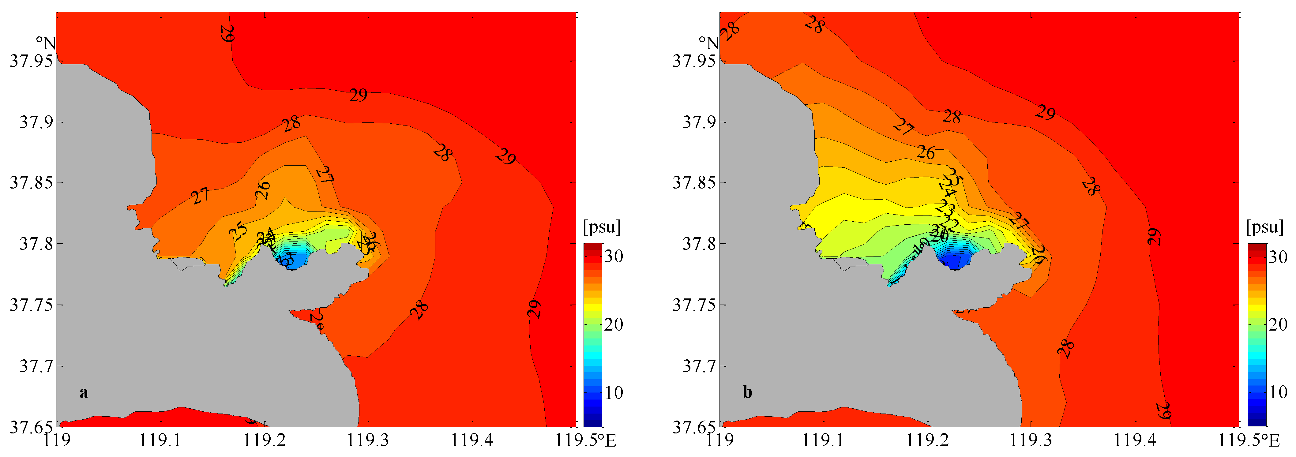
The area around the YR Estuary has a prevailing southern wind in summer. Four cases (cases 3–6) with different wind speeds were established to explore the influence of summer monsoons on salinity diffusion around the YR Estuary. Figure 13 shows the corresponding diffusion distribution of surface salinity. When there was no wind (case 3), under the action of tide and residual current, more fresh water from the YR was imported into LZB. When there was a breeze (v = 4 m/s) (case 4), the southward area with low salinity decreased obviously. Under the effect of surface currents and thermal stratification [19], fresh water from the YR began to spread to the middle of the BHS. When the southern wind continued to strengthen (case 5 and case 6), the diffusion trend of low salinity water to the middle of BH Bay was strengthened. When strong wind increased, the YR’s diluted water diffused almost completely northward. Generally speaking, the diffusion direction of the YR plume was roughly counterclockwise from south to north with the strengthening of the wind during the wet season.
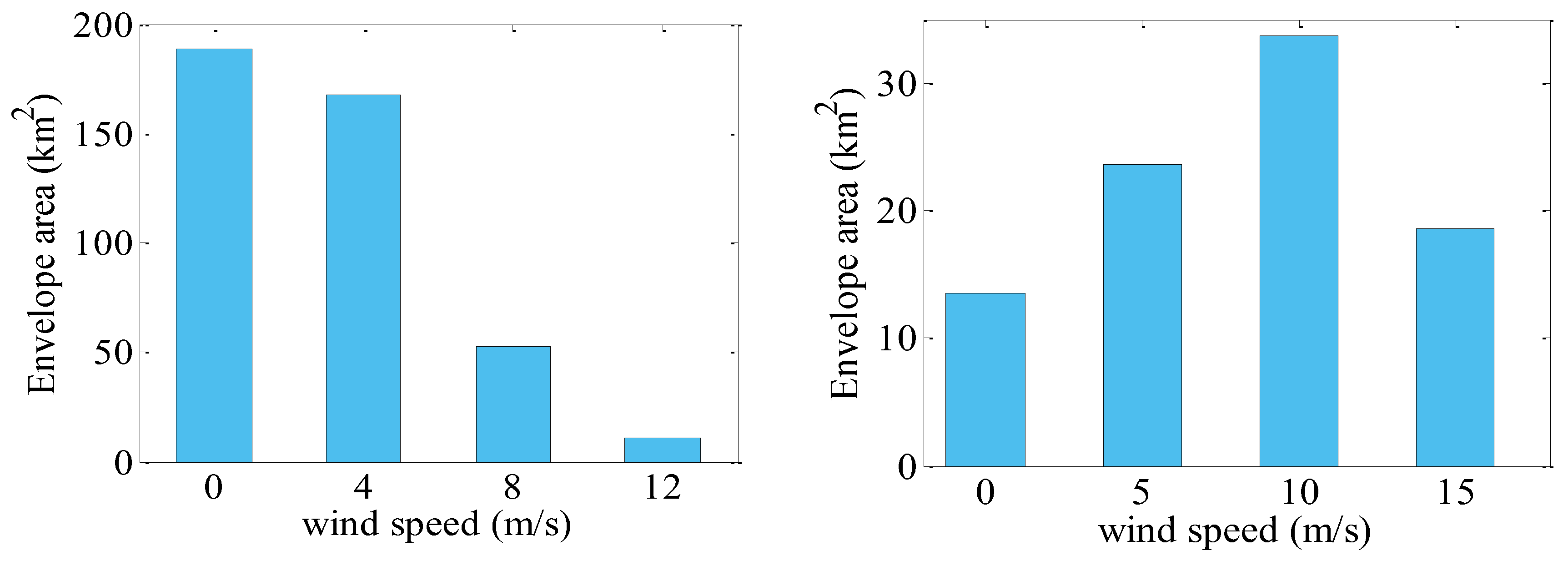
Figure 14 shows the vertical salinity diffusion in the range of 37.7° N–38.6° N at the section of 119.25° E. When the wind speed was low (case 3 and case 4), there were more horizontal layers of salinity, and low salinity water diffused a longer distance. Figure 15 shows the statistical diagram of surface area of 27 psu isohaline in the wet and dry seasons under different wind speeds. When the wind speed increased, the surface area of low-salinity water became smaller and smaller. When the wind speed was over 4 m/s, the area of low salinity water began to decrease sharply. Wind facilitated vertical exchange of salinity. Along the same horizontal length, the higher the wind speed was, the more complete the exchange of water with different densities was.
4.3. Influence of Different Wind Speeds on Salinity Diffusion in the Dry Season
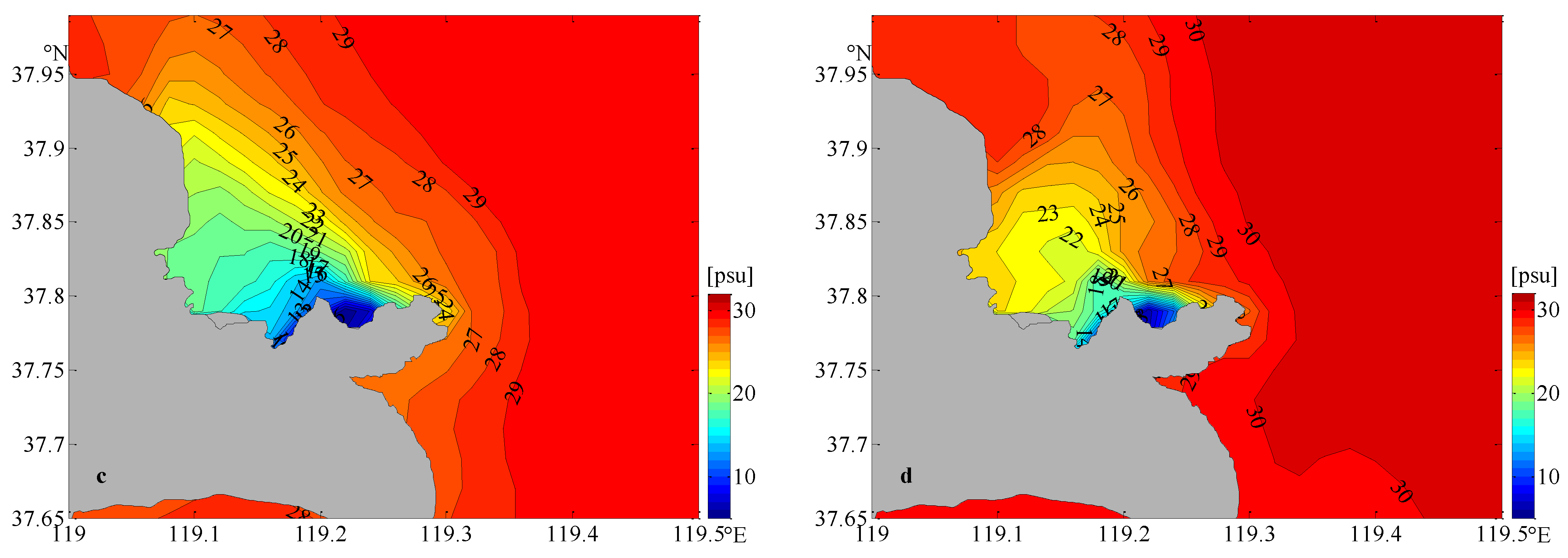
Northern wind prevails in winter in the estuary of the YR. In order to explore the influence of different wind speeds on salinity diffusion during the dry season, the northeasterly wind with the highest statistical frequency was selected as the constant wind direction, and four different gradient wind speeds were set (case 7–10). Figure 16 shows the surface salinity distribution at different wind speeds during the dry season, and Figure 17 shows the salinity distribution profile at a section of 119.25° E. Due to limited river discharge during the dry season, the plume only distributed in the water near the estuary of the YR. Under the influence of the northeastern wind, the diffusion of fresh water from the YR to the sea was restrained. Influenced by the direction of the estuary, the low-salinity plume spread northwest along the shore. The area with low salinity in the dry season showed that northeasterly wind promoted the diffusion of the plume even under low wind speed, causing an increase in the plume’s scope and area. When the strong wind speed continued to increase, the water area with low salinity began to decrease. This was mainly related to runoff and the prevailing wind direction in the dry season. Due to low runoff, wind played a leading role in salinity diffusion in the dry season. When the wind speed was low, the wind promoted the diffusion of fresh water from the YR to the northwest; when the wind strengthened, the vertical diffusion was more obvious. Changes in the profile corresponding to the wind speed also indicated that vertical diffusion became more intense and the surface area began to decrease when wind strengthened.
5. Conclusions
The YR’s discharge was 2.6 times higher than in previous years, and wind was stronger than ever during the wet season in 2020, which was particularity different from the statistical results of previous years. In this paper, the FVCOM three-dimensional model was used to simulate salinity diffusion around the estuary of the YR during the wet and dry seasons in 2020. The effects of river discharge and wind speed on salinity diffusion were also investigated. Under the influence of residual current and the direction of ebb and flow, fresh water from the YR diffusing to LZB can last for a long time. Under the influence of monsoons, the salinity diffusions in the wet and dry seasons were obviously different. In the wet season, the plume of low-salinity water spread southward, and the YR’s diluted water affected nearly the entire LZB. The salinity front of 27 psu could reach the central part of LZB, and the envelope area of 27 psu isohaline accounted for about one-quarter of the total LZB. In the dry season, due to limited river discharge, low salinity water only concentrated near the estuary of the YR. In addition, the fresh water could directly affect the offshore seabed.
The discharge from the river mainly affected the area, distance, and depth of salinity diffusion. Wind could change the structure and direction of the plume diffusion. In the wet season, under the action of the southern wind, with the strengthening of the wind, the diffusion direction of the YR’s plume was roughly counterclockwise from south to north. The envelope area of the 27 psu isohaline gradually decreased with increasing wind speed. In the dry season, with the increase of wind speed and the limited northeasterly wind and river discharge, the YR’s plume spread northwest along the nearshore. Wind speed under 10 m/s was positively correlated with the envelope area of the 27 psu isohaline, and the surface plume area began to decrease only at a wind speed above 10 m/s.
The model developed and the results from this study provide valuable information for establishing robust water resource regulations for the YR. This is particularly important to ensure that the areas with low salinity in the YR Estuary will not decrease and affect the reproduction of fish species. The present study only considered the effects of wind speed and runoff, but did not take the effects of waves into account. In the real ocean, waves play an important role in turbulence. Moreover, previous studies [35] have shown that hyporheic exchange also plays an important role in mixing. Therefore, the influence of waves and hyporheic exchange can be considered in future research.
Author Contributions
Methodology, H.S.; Software, H.Q. and S.Q.; Formal analysis, H.S.; Investigation, Q.L.; Resources, Y.G.; Data curation, Y.G.; Writing—original draft, H.Q. All authors have read and agreed to the published version of the manuscript.
Funding
This work was supported by the Major Research Grant (No. U1906231) from the Natural Science Foundation of China (NSFC) and the Natural Science Foundation of China (No. 51909114).
Data Availability Statement
Data are available from the corresponding author upon reasonable request.
Conflicts of Interest
The authors declare no conflict of interest.
References
- Xing, Y.; Ai, C.F.; Jin, S. A three-dimensional hydrodynamic and salinity transport model of estuarine circulation with an application to a macrotidal estuary. Appl. Ocean Res. 2013, 39, 53–71. [Google Scholar] [CrossRef]
- Dong, L.X.; Su, J.L.; Wong, L.A.; Cao, Z.; Chen, J.C. Seasonal variation and dynamics of the Pearl River plume. Cont. Shelf Res. 2004, 24, 1761–1777. [Google Scholar] [CrossRef]
- Xia, M.; Xie, L.; Leonard, J.; Pietrafesa, L.J. Modeling of the Cape Fear River Estuary plume. Geophys. Res. Lett. 2007, 30, 698–709. [Google Scholar] [CrossRef]
- Granskog, M.A.; Ehn, J.; Niemel, M. Characteristics and potential impacts of under-ice river plumes in the seasonally ice-covered Bothnian Bay (Baltic Sea). J. Mar. Syst. 2005, 53, 187–196. [Google Scholar] [CrossRef]
- Restrepo, J.C.; Schrottke, K.; Bartholomae, A.; Ospino, S.; Ortíz, J.C.; Orejarena, A. Estuarine and sediment dynamics in a microtidal tropical estuary of high fluvial discharge: Magdalena River (Colombia, South America). Mar. Geol. 2018, 398, 86–98. [Google Scholar] [CrossRef]
- Pritchard, M.; Huntley, D.A. A simplified energy and mixing budget for a small river plume discharge. J. Geophys. Res. Ocean 2006, 111, C3. [Google Scholar] [CrossRef]
- Walker, N.D.; Wiseman, W.J.; Rouse, L.J.; Babin, A. Effects of River Discharge, Wind Stress, and Slope Eddies on Circulation and the Satellite-Observed Structure of the Mississippi River Plume. J. Coast. Res. 2005, 216, 1228–1244. [Google Scholar] [CrossRef]
- Molleri, G.S.F.; Novo, E.M.L.d.M.; Kampel, M. Space-time variability of the Amazon River plume based on satellite ocean color. Cont. Shelf Res. 2010, 30, 342–352. [Google Scholar] [CrossRef]
- Kourafalou, V.H. river plume development in semi-enclosed mediterranean regions: North adriatic sea and northwestern aegean sea. J. Marrine Syst. 2001, 30, 181–205. [Google Scholar] [CrossRef]
- Fong, D.A.; Geyre, W.R. The alongshore transport of freshwater in a surface-trapped river plume. J. Phys. Oceanogr. 2002, 32, 957–972. [Google Scholar] [CrossRef]
- Cheng, R.T.; Casulli, V. Modeling a three-dimensional river plume over continental shelf using a 3D unstructured grid model. In Estuarine and Coastal Modeling; ASCE: Reston, VA, USA, 2004. [Google Scholar]
- Wang, F.; Meng, Q.; Tang, X.; Hu, D. The long-term variability of sea surface temperature in the seas east of China in the past 40 a. Acta Oceanol. Sin. 2013, 32, 48–53. [Google Scholar] [CrossRef]
- Zhou, J.H.; Matthew, J.; Deitcha, S.G.; Screaton, E.J.; Olabarrieta, M. Effect of Mississippi River discharge and local hydrological variables on salinity of nearby estuaries using a machine learning algorithm—ScienceDirect. Estuar. Coast. Shelf Sci. 2021, 263, 107628. [Google Scholar] [CrossRef]
- Salmela, J.; Kasvi, E.; Alho, P. River plume and sediment transport seasonality in a non-tidal semi-enclosed brackish water estuary of the Baltic Sea. Estuar. Coast. Shelf Sci. 2020, 245, 106986. [Google Scholar] [CrossRef]
- Coogan, J.; Dzwonkowski, B. Observations of Wind Forcing Effects on Estuary Length and Salinity Flux in a River-Dominated, Microtidal Estuary, Mobile Bay, Alabama. J. Phys. Oceanogr. 2018, 48, 1787–1802. [Google Scholar] [CrossRef]
- Abolfathi, S.; Pearson, J.M. Solute dispersion in the nearshore due to oblique waves. In Proceedings of the 34th Conference on Coastal Engineering, Seoul, Republic of Korea, 15–20 June 2014; ISBN 9780989661126. [Google Scholar] [CrossRef] [Green Version]
- Zeinabi, A.; Kohansal, A. Numerical modeling of sediment transport patterns under the effects of waves and tidal currents at Pars port complex inlet. Int. J. Marit. Technol. 2020, 14, 33–40. [Google Scholar]
- Xu, J.X. The Water Fluxes of the Yellow River to the Sea in the Past 50 Years, in Response to Climate Change and Human Activities. Environ. Manag. 2005, 35, 620. [Google Scholar]
- Wang, Q.; Guo, X.; Takeoka, H. Seasonal variations of the Yellow River plume in the Bohai Sea: A model study. J. Geophys. Res. 2008, 113, C08046. [Google Scholar] [CrossRef]
- Mao, X.Y.; Jiang, W.; Zhao, P.; Gao, H. A 3-D numerical study of salinity variations in the Bohai Sea during the recent years. Cont. Shelf Res. 2008, 28, 2689–2699. [Google Scholar] [CrossRef]
- Lin, C.; Su, J.L.; Xu, B.R.; Tang, Q. Long-term variations of temperature and salinity of the Bohai Sea and their influence on its ecosystem. Prog. Oceanogr. 2001, 49, 7–19. [Google Scholar] [CrossRef]
- Wang, Y.; Liu, Z.H.; Gao, H.W.; Guo, X. Response of salinity distribution around the Yellow River mouth to abrupt changes in river discharge. J. Cont. Shelf Res. 2011, 31, 685–694. [Google Scholar] [CrossRef]
- Sui, Y.; Shi, H.Y.; You, Z.J.; Qiao, S.; Sun, J. Long-term Trend and Change Point Analysis on Runoff and Sediment Flux into the Sea from the Yellow River during the Period of 1950–2018. J. Coast. Res. 2020, 99, 203. [Google Scholar] [CrossRef]
- Liu, H. Fate of three major rivers in the Bohai Sea: A model study. Cont. Shelf Res. 2011, 31, 1490–1499. [Google Scholar] [CrossRef]
- Shi, H.Y.; Li, Q.J.; Sun, J.C.; Gao, G.; Sui, Y.; Qiao, S.; You, Z. Variation of Yellow River Runoff and Its Influence on Salinity in Laizhou Bay. J. Ocean. Univ. China 2020, 19, 1235–1244. [Google Scholar] [CrossRef]
- Cheng, X.Y.; Zhu, J.R.; Chen, S.L. Extensions of the river plume under various Yellow River courses into the Bohai Sea at different times. Estuar. Coast. Shelf Sci. 2020, 249, 107092. [Google Scholar] [CrossRef]
- Chen, C.S.; Beardsley, R.C. An Unstructured Grid, Finite-Volume Coastal Ocean Model. In FVCOM User Manual, 2nd ed.; SMAST/UMASSD: New Bedford, MA, USA, 2006; pp. 1–135. [Google Scholar]
- Chen, C.S.; Liu, H.D.; Robert, C. An Unstructured Grid, Finite-Volume, Three-dimensional, primitive equations ocean model: Application to Coastal and Estuaries. J. Atmos. Ocean. 2003, 20, 159–186. [Google Scholar] [CrossRef]
- Li, S.; Chen, C. Air-sea interaction processes during hurricane Sandy: Coupled WRF-FVCOM model simulations. Prog. Oceanogr. 2022, 206, 102855. [Google Scholar] [CrossRef]
- Chen, C.; Huang, H.; Lin, H.; Blanton, J.; Li, C.; Andrade, F. A Wet/Dry Point Treatment Method of FVCOM, Part II: Application to the Okatee/Colleton River in South Carolina. J. Mar. Sci. Eng. 2022, 10, 982. [Google Scholar] [CrossRef]
- Yang, Z.; Shao, W.; Ding, Y.; Shi, J.; Ji, Q. Wave Simulation by the SWAN Model and FVCOM Considering the Sea-Water Level around the Zhoushan Islands. J. Mar. Sci. Eng. 2020, 8, 783. [Google Scholar] [CrossRef]
- Goodarzi, D.; Mohammadian, A.; Pearson, J.; Abolfathi, S. Numerical modelling of hydraulic efficiency and pollution transport in waste stabilization ponds. Ecol. Eng. 2022, 182, 106702. [Google Scholar] [CrossRef]
- Goodarzi, D.; Abolfathi, S.; Borzooei, S. Modelling solute transport in water disinfection systems: Effects of temperature gradient on the hydraulic and disinfection efficiency of serpentine chlorine contact tanks. J. Water Process. Eng. 2020, 37, 101411. [Google Scholar] [CrossRef]
- SL 160-2012; Regulation for Hydraulic and Thermal Model in Cooling Water Projects. Ministry of Water Resources of the People’s Republic of China: Beijing, China, 2017.
- Cook, S.; Price, O.; King, A.; Finnegan, C.; van Egmond, R.; Schafer, H.; Pearson, J.M.; Abolfathi, S.; Bending, G.D. Bedform characteristics and biofilm community development interact to modify hyporheic exchange. Sci. Total Environ. 2020, 749, 141397. [Google Scholar] [CrossRef]
Figure 1.
The locations of the Yellow River and Lijin station (a) and annual runoff of the Yellow River from 1952 to 2017 (b).
Figure 1.
The locations of the Yellow River and Lijin station (a) and annual runoff of the Yellow River from 1952 to 2017 (b).

Figure 2.
Grid information for the research area.

Figure 3.
River discharge statistics in the wet season (a) and the dry season (b) in 2020 and 2007–2017 (wet season: 1 July–31 August; dry season: 1 January–28 February; data link: http://61.163.88.227:8006/hwsq.aspx?sr=0nkRxv6s9CTRMlwRgmfFF6jTpJPtAv87, accessed on 29 March 2023).
Figure 3.
River discharge statistics in the wet season (a) and the dry season (b) in 2020 and 2007–2017 (wet season: 1 July–31 August; dry season: 1 January–28 February; data link: http://61.163.88.227:8006/hwsq.aspx?sr=0nkRxv6s9CTRMlwRgmfFF6jTpJPtAv87, accessed on 29 March 2023).

Figure 4.
Wind rose in the wet season (right) and the dry season (left) in 2020 (a,b) and 2007–2017 (c,d) (wet season: 1 July–31 August; dry season: 1 January–28 February; data link: https://www.ecmwf.int/en/forecasts/datasets/reanalysis-datasets/era5, accessed on 29 March 2023).
Figure 4.
Wind rose in the wet season (right) and the dry season (left) in 2020 (a,b) and 2007–2017 (c,d) (wet season: 1 July–31 August; dry season: 1 January–28 February; data link: https://www.ecmwf.int/en/forecasts/datasets/reanalysis-datasets/era5, accessed on 29 March 2023).

Figure 5.
Station information of observations (tide and current: H1–H6; salinity: S1 and S2).

Figure 6.
Verification of tidal level.

Figure 7.
Verification of tidal current.


Figure 8.
Verification of salinity in the dry (left) and wet (right) period.

Figure 9.
Distribution of the surface residual current field in the wet season (a) and the dry season (b).
Figure 9.
Distribution of the surface residual current field in the wet season (a) and the dry season (b).

Figure 10.
Distribution of surface (right) and bottom (left) salinity in the wet (top) and dry (bottom) seasons.
Figure 10.
Distribution of surface (right) and bottom (left) salinity in the wet (top) and dry (bottom) seasons.

Figure 11.
Salinity vertical distribution in Laizhou Bay during the wet season (left) and the dry season (right).
Figure 11.
Salinity vertical distribution in Laizhou Bay during the wet season (left) and the dry season (right).

Figure 12.
Surface (top) and vertical (bottom) salinity distribution of case 1 (left) and case 2 (right).
Figure 12.
Surface (top) and vertical (bottom) salinity distribution of case 1 (left) and case 2 (right).

Figure 13.
Surface salinity distribution at different wind speeds in the wet season. ((a): case 3, (b): case 4, (c): case 5, (d): case 6).
Figure 13.
Surface salinity distribution at different wind speeds in the wet season. ((a): case 3, (b): case 4, (c): case 5, (d): case 6).

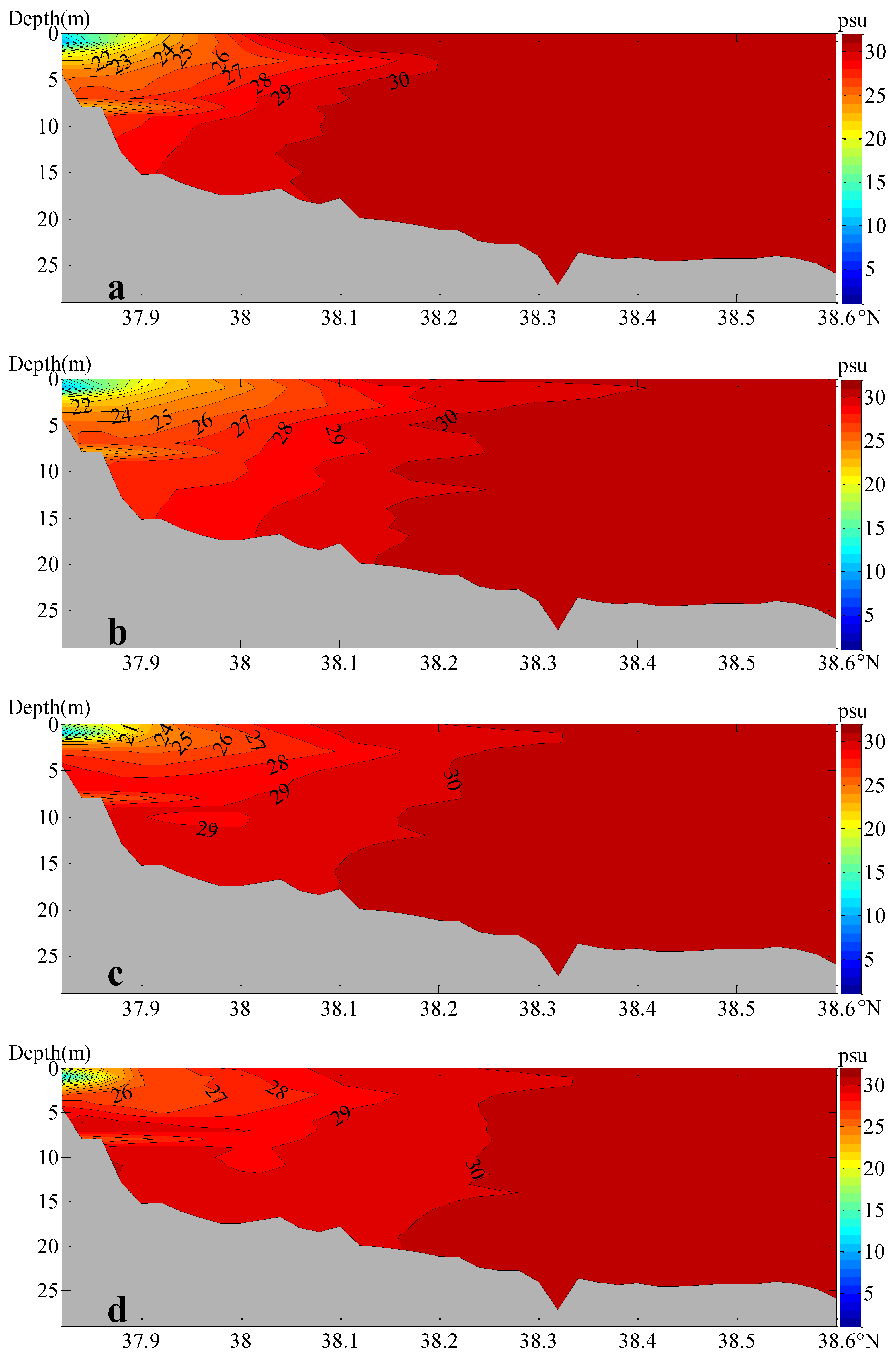
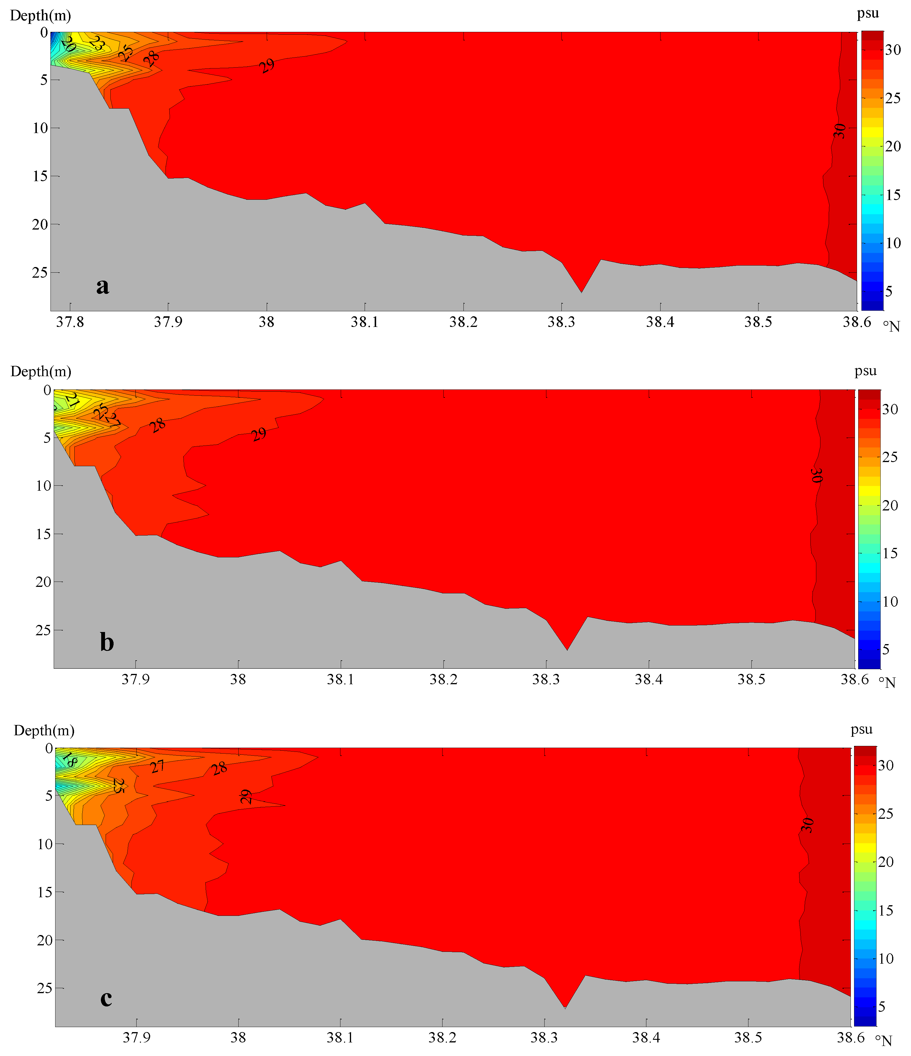
Figure 14.
Vertical salinity distribution at different wind speeds in the wet season ((a): case 3, (b): case 4, (c): case 5, (d): case 6).
Figure 14.
Vertical salinity distribution at different wind speeds in the wet season ((a): case 3, (b): case 4, (c): case 5, (d): case 6).

Figure 15.
Surface area of 27 psu isohaline in the wet season (right) and the dry season (left).

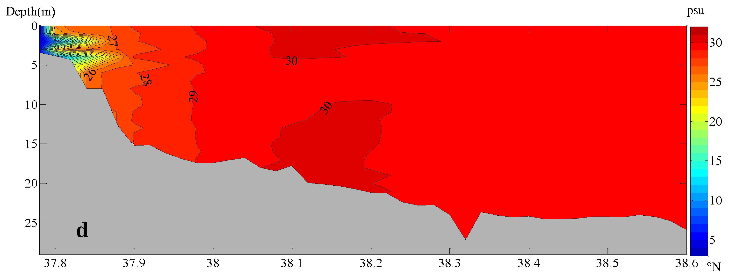
Figure 16.
Surface salinity distribution at different wind speeds in the dry season ((a): case 3, (b): case 4, (c): case 5, (d): case 6).
Figure 16.
Surface salinity distribution at different wind speeds in the dry season ((a): case 3, (b): case 4, (c): case 5, (d): case 6).


Figure 17.
Vertical salinity distribution at different wind speeds in the dry season ((a): case 3, (b): case 4, (c): case 5, (d): case 6).
Figure 17.
Vertical salinity distribution at different wind speeds in the dry season ((a): case 3, (b): case 4, (c): case 5, (d): case 6).


Table 1.
Detailed information of the observation stations.
| Station Type | Station Name | Longitude | Latitude | Time |
|---|---|---|---|---|
| Tidal current and tide | H1 | 119.077247 | 38.207694 | 10 October 2018–11 October 2018 |
| H2 | 119.322183 | 37.885078 | 10 October 2018–11 October 2018 | |
| H3 | 119.535017 | 37.603250 | 10 October 2018–11 October 2018 | |
| H4 | 119.751378 | 38.539094 | 10 October 2018–11 October 2018 | |
| H5 | 119.987794 | 38.236428 | 10 October 2018–11 October 2018 | |
| H6 | 120.212142 | 37.935142 | 10 October 2018–11 October 2018 | |
| Salinity | S1 | 118.99837 | 38.08946 | 20 February–28 February 2020, 20 August–27 February |
| S2 | 120.25612 | 37.64275 | 20 February–28 February 2020, 20 August–27 February |
Table 2.
Correlation coefficients (r) between simulation and measured values.
| Station | Tide | Surface (V) | Surface (D) | Middle (V) | Middle (D) | Bottom (V) | Bottom (D) | Dry | Wet |
|---|---|---|---|---|---|---|---|---|---|
| H1 | 0.47 | 0.94 | 0.87 | 0.96 | 0.98 | 0.96 | 0.98 | - | - |
| H2 | 0.97 | 0.93 | 0.76 | 0.94 | 0.99 | 0.90 | 0.99 | - | - |
| H3 | 0.98 | 0.67 | 0.98 | 0.74 | 0.98 | 0.77 | 0.98 | - | - |
| H4 | 0.99 | 0.93 | 1.00 | 0.93 | 1.00 | 0.89 | 1.00 | - | - |
| H5 | 0.99 | 0.82 | 0.99 | 0.81 | 0.99 | 0.77 | 0.99 | - | - |
| H6 | 0.98 | 0.91 | 1.00 | 0.93 | 1.00 | 0.88 | 0.99 | - | - |
| S1 | - | - | - | - | - | - | - | 0.60 | 0.47 |
| S2 | - | - | - | - | - | - | - | 0.73 | 0.65 |
Table 3.
Description of numerical experiments.
| Case | Period | River Discharge | Wind |
|---|---|---|---|
| 1 | wet season | Average daily river discharge from 2007 to 2017 | Hourly variation |
| 2 | wet season | Average daily river discharge in 2020 | Hourly variation |
| 3 | wet season | None | |
| 4 | wet season | Constant wind, south with speed of 4 m/s | |
| 5 | wet season | Constant wind, south with speed of 8 m/s | |
| 6 | wet season | Constant wind, south with speed of 12 m/s | |
| 7 | dry season | None | |
| 8 | dry season | Constant wind, northeast with speed of 5 m/s | |
| 9 | dry season | Constant wind, northeast with speed of 10 m/s | |
| 10 | dry season | Constant wind, northeast with speed of 15 m/s |
Disclaimer/Publisher’s Note: The statements, opinions and data contained in all publications are solely those of the individual author(s) and contributor(s) and not of MDPI and/or the editor(s). MDPI and/or the editor(s) disclaim responsibility for any injury to people or property resulting from any ideas, methods, instructions or products referred to in the content. |
© 2023 by the authors. Licensee MDPI, Basel, Switzerland. This article is an open access article distributed under the terms and conditions of the Creative Commons Attribution (CC BY) license (https://creativecommons.org/licenses/by/4.0/).
Share and Cite
MDPI and ACS Style
Qin, H.; Shi, H.; Gai, Y.; Qiao, S.; Li, Q. Sensitivity Analysis of Runoff and Wind with Respect to Yellow River Estuary Salinity Plume Based on FVCOM. Water 2023, 15, 1378. https://0-doi-org.brum.beds.ac.uk/10.3390/w15071378
AMA Style
Qin H, Shi H, Gai Y, Qiao S, Li Q. Sensitivity Analysis of Runoff and Wind with Respect to Yellow River Estuary Salinity Plume Based on FVCOM. Water. 2023; 15(7):1378. https://0-doi-org.brum.beds.ac.uk/10.3390/w15071378
Chicago/Turabian StyleQin, Huawei, Hongyuan Shi, Yunyun Gai, Shouwen Qiao, and Qingjie Li. 2023. "Sensitivity Analysis of Runoff and Wind with Respect to Yellow River Estuary Salinity Plume Based on FVCOM" Water 15, no. 7: 1378. https://0-doi-org.brum.beds.ac.uk/10.3390/w15071378
Note that from the first issue of 2016, this journal uses article numbers instead of page numbers. See further details here.