Article

Identification of Microplastics Using µ-Raman Spectroscopy in Surface and Groundwater Bodies of SE Attica, Greece

1
School of Mining and Metallurgical Engineering, Division of Geo-Sciences, National Technical University of Athens, 15773 Zografou, Greece
2
Mineralogy-Geology Laboratory, Department of Natural Resources and Agricultural Engineering, Agricultural University of Athens, 11855 Athens, Greece
3
Université Claude Bernard Lyon 1, LEHNA UMR 5023, CNRS, ENTPE, F-69622 Villeurbanne, France
*
Author to whom correspondence should be addressed.
Submission received: 31 January 2024 / Revised: 11 March 2024 / Accepted: 12 March 2024 / Published: 14 March 2024

Abstract

:
Sixteen surface (5) and groundwater (11) samples were collected from the south-eastern part of Attica, Greece, and analysed for physico-chemical parameters and microplastics (MPs) by optical microscopy and Raman microspectroscopy (RS). A total of 3399 particles were optically identified in all sixteen samples, ranging from only 16 particles/L in a sample from a deeper borehole to 513 particles/L in a sample from a shallow water well. They were then visually classified into eight categories based on their color, texture, size, reflectivity, shape, and general morphological properties. Raman microspectroscopy was performed on the particles on the filters and revealed four different types of MPs, namely polyethylene (PE, 35%), polypropylene (PP, 30%), polystyrene (PS, 10%), and polyethylene terephthalate (PET, 25%). The samples from the shallow phreatic aquifer contained more MPs than the samples from the deeper borehole, which contained fewer MPs and categories. This is to be expected, since the phreatic aquifer (a) is generally more contaminated, as it is close to human activities that generate MPs and its infiltration depth is only a few metres, which means that many microplastics can infiltrate at such shallow depths, and (b) it is exposed to the atmosphere, so they can also be suspended in the air. On the other hand, it is interesting to note that MPs, especially PET and PE, were detected in the borehole sample, suggesting that MPs can migrate to greater depths through water infiltration. Chemical analyses of the groundwater samples revealed high values of E.C., Ca2+, Mg2+, Cl, and Na+, which indicate that seawater intrusion is taking place in the coastal aquifer system of the Erasinos basin. The increased concentrations of NO3 and PO43− also indicate the impact of agricultural activities.

1. Introduction

Environmental geochemistry is an important application of Raman spectroscopy (RS) in the geosciences. From inorganic to organic and biological contaminants in soil, water and air, RS is an important tool for their characterization. In the last decade, RS has been successfully used to identify microplastics (MPs) [1,2]. “Microplastics” were defined as plastic particles smaller than 5 mm by the National Oceanic and Atmospheric Administration (NOAA) International Research Workshop on the occurrence, effects, and fate of microplastic marine debris (2009, [3]). Since then, MPs have been systematically detected in soils, sediments, and in marine and aquatic environments around the world, raising scientific interest and public health concerns [4]. The main types of polymers that can be detected in the environment are polyethylene (PE), polypropylene (PP), and polystyrene (PS). Microplastics are either primary MPs, which include production pellet nurdles and microbeads, or secondary MPs, which are formed by the mechanical and chemical decomposition of larger plastic waste and fibers from synthetic textiles [5]. Although MPs are mostly colorless, colored MPs are also frequently found. This is due to the increasing trend of adding color pigments to plastics to obtain more attractive plastic products or to absorb part of the ultraviolet light as a light stabilizer to prevent or delay photodegradation and thus extend the life of plastic products [6].
From the Mediterranean [7] to the Pacific Ocean [8], Arctic Sea ice [9], and freshwater lakes [10], MPs are reported in an increasing number of studies worldwide.
The identification of MPs is of great significance and follows the process of separation, extraction, or concentration. The physicochemical properties of MPs, such as size, shape, and composition, are crucial for studying their pathways in soil, marine, and aquatic environments. Microscopic methods such as optical microscopy and scanning electron microscopy mainly provide information on the size, color, and shape of the MPs, whereas the vibrational spectroscopic analytical methods, Fourier Transform Infrared Spectroscopy (FT-IR) and RS, are employed to reveal the chemical composition of the MPs [11]. More advanced analytical methods such as Flow Cytometry (FCM), Dynamic Light Scattering (DLS), hyperspectral imaging (HIS), and Atomic Force Microscopy (AFM) have also been applied to the study of MPs [12,13,14] and others have yet to be adopted.
Capable of detecting MPs with particle sizes as small as 1 μm [15], RS spectroscopy combined with an RS microscope (µ-RS) offers rapid, generally non-destructive analysis and is becoming a conventional tool in MPs identification, as evidenced by the rapidly growing number of related publications. Raman imaging has also been applied in identifying MPs on filters [16].
Identifying the type of MPs found in soils and waters provides information on the origin of MPs, as well as the weathering/degradation processes that follow the original deposition/release. This may further contribute to monitoring and assessing the different types of MPs in the environment, setting up future prevention measures.
Even though MPs are considered a significant factor in groundwater pollution, a limited number of studies have linked them to other quality parameters such as electric conductivity (EC), pH, temperature (T), dissolved oxygen (DO), oxidation–reduction potential (ORP), total dissolved solids (TDS), turbidity, and salinity. Measuring and assessing these physical parameters in situ could improve the determination of the sources and behavior of MPs as a contaminant in aquifer systems [17]. However, the existing knowledge on how these parameters affect water or interact with MPs is still very limited. It is assumed that microplastics adsorb and transfer organic pollutants and ionic heavy metal pollutants (e.g., Cu, Pb, Hg, Cd, and Cr) in the aquatic environment [18]. The adsorption process of MPs is also controlled by various anions and cations [19]. It is believed that the physical parameters and chemical composition of groundwater are important factors influencing the occurrence of MPs in groundwater [17]. In the coming years, the big challenge for researchers will be the following: how do MPs interact with the chemical composition of groundwater and other contaminants?
There are only a limited number of published studies on the occurrence of MPs in Greek marine and aquatic ecosystems, mostly focussing on seawater samples and sediments. The analytical methods of SEM and ATR-FTIR have been mainly used to study the degradation of plastic materials in different marine environments in Greece [20], plastic pellets and fragments of polyethylene (PE) and expanded polystyrene (EPS) from two beaches of Salamina Island [21], and PE and PP as ingested microplastics in Boops Boops fish in the Southern Ionian Sea and Saronikos Gulf [22]. In addition, the temporal and spatial distribution of plastic pellets and fragments on nine sandy beaches along the coast of Northern Crete was investigated using Gas Chromatography—Ion Trap Mass Spectrometry (GC-ITMS) [23]. However, the possible presence of MPs in groundwater from wells and boreholes in Greece has yet to be explored, limiting our knowledge to the coastal and marine environment.
In this work, we conducted a thorough investigation of MPs detected in the surface water and groundwater of the Erasinos River basin in the southeastern part of Attica, Greece, using RS, after filtering and detailed visual presorting. In addition, chemical analyses of water samples were also carried out, in order to investigate the relationship between the chemical status of the groundwater and the occurrence of MPs in the Erasinos basin. The study area was selected because it is characterized by certain anthropogenic activities and land uses (Eleftherios Venizelos International Airport, with more than 25 million passengers annually, large shopping malls). In the Erasinos basin, there are also a variety of potential sources of MPs entering the groundwater system, such as surface runoff, agricultural activities (agrochemical products), atmospheric deposition, and wastewater, which can contribute to MP contamination. The aim was to determine the morphological characteristics and type(s) of MPs present, the impact of degradation, and the possible dependence on the depth of the aquifer. This will further contribute to build up a database of MPs present in Greek ecosystems, including underground aquifers of different types and depths.

2. Materials and Methods
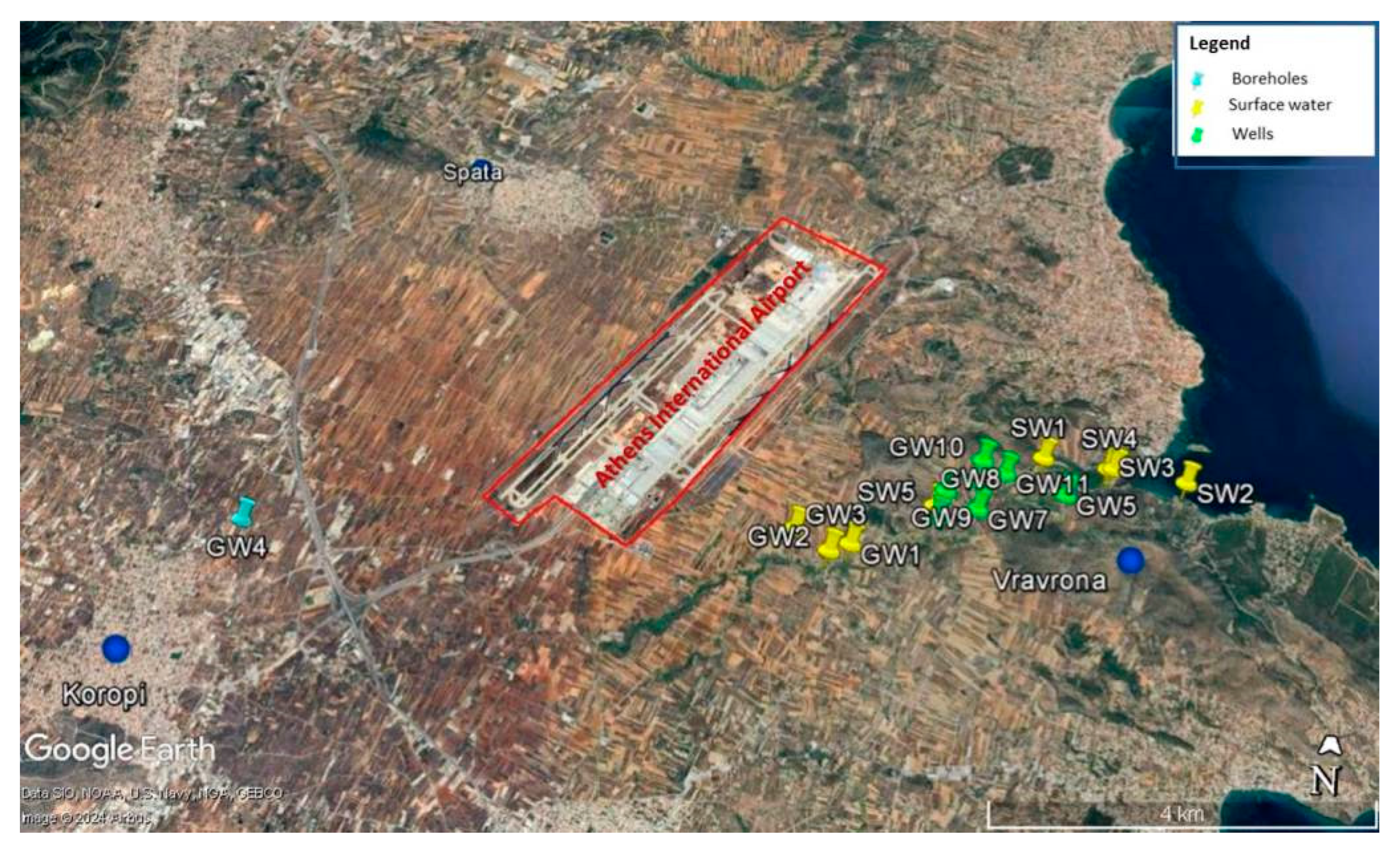
2.1. Study Area

The study area of the Erasinos basin is located in the south-eastern part of Attica Prefecture, covering an area of approximately 204 km2. The basin is bordered to the east by the coastline of Rafina–Artemis–Porto Rafti. The Erasinos River flows into the southern Gulf of Evoikos. The climate of the region is characterized by low precipitation and high summer temperatures. The average annual precipitation is estimated at 406 mm per year.
The Erasinos basin is part of the Attico-Cycladic Massif. The dominant geological formations in the basin are as follows [24,25] (Figure 1): (a) the crystalline basement of Paleozoic–Upper Cretaceous age (schists and carbonate rocks, mainly limestones and dolomite marbles), and (b) the clastic depositions of Neogene and Quaternary age (marl limestones, marls, clays, sandstones, conglomerates, and other unconsolidated materials).
A knowledge of the hydrogeological conditions of the basin is a crucial factor for the migration of MPs. In general, the groundwater flows towards the sea and discharges into Vavrona bay, while in some parts of the basin, it flows into the Erasinos River [26]. The groundwater flow is locally determined mainly by impermeable schists.
The main aquifer systems in the area are the following [27]:
  • A karstic aquifer with a high capacity (discharge rate over 100 m3/h) as it is also fractured. Along the coasts of Porto Rafti and Artemis, scattered underwater sources of this karst water have been identified, confirming the hydraulic connection with seawater.
  • The alternation of permeable and impermeable layers favors the development of unconfined and confined aquifers in the Neogene deposits. The capacity of these systems is low (discharge rates up to 5 m3/h). The shallow aquifer is overexploited by extensive pumping to meet irrigation and industrial needs in the region.
  • A phreatic aquifer has developed in Quaternary deposits with low capacity (discharge rates of 15 up to 35 m3/h). The phreatic aquifer is exploited by many wells, resulting in seawater intrusion in the coastal parts of the aquifer system. This fact is also reflected in the groundwater quality, as it is characterized as brackish.
  • Fractured aquifers are mainly developed in the Rafina area, due to secondary porosity, created by metamorphic and tectonic processes and the weathering of impermeable formations.
The main recharge of the aquifer system, investigated here, originates from the following: (a) direct infiltration of precipitation and (b) infiltration of surface runoff, rivers, and streams, and (c) lateral recharge from other aquifer systems that are hydraulically connected.
Land uses are mainly as follows: (i) agriculture, (ii) industry, (iii) pastures, (iv) transportation (Eleftherios Venizelos International Airport), (v) residential, and (vi) commercial.
The area is intensively used for agriculture, resulting in aquifer degradation, with significant concentrations of inorganic pollutants such as NO3, NO2, and PO43−. In addition, high concentrations of sodium (Na+) and chlorine (Cl) are also traced due to seawater intrusion from excessive pumping [26,27]. The area is also exposed to significant pollution from plastic materials due to intensive agriculture and anthropogenic processes, such as the Eleftherios Venizelos International Airport and the neighbouring city of Koropi.
Figure 1. Geological map of the Erasinos basin, with the locations of the surface and groundwater samples studied here (modified from the 1:50,000 geological map published by the Institute of Geology and Mineral Exploration of Greece [28]).
Water 16 00843 g001

2.2. Sampling

Sixteen (16) samples were collected in August 2020 from surface waters, groundwater wells, and a borehole from the catchment area of the Erasinos River in the area of Vravrona and Koropi; five (5) from surface waters (SW1, SW2, SW3, SW4, SW5), one (1) of which (SW2) was from the river exit into the sea, ten (10) from wells (GW1, GW2, GW3, GW5, GW6, GW7, GW8, GW9, GW10, GW11), and one (1) from a water borehole (GW4) (Figure 2). All groundwater samples, except GW4, were collected from the phreatic water table (up to 8 m), and the surface water samples SW1, SW3, SW4, and SW5 were collected from the Erasinos River estuary. Borehole sample GW4 was taken from a deeper aquifer (70 m) within the Neogene sediments. In all cases, the water was used exclusively for irrigation purposes. The sampling sites are presented in Table 1. The water samples were collected in two 500 mL glass bottles for microplastic analysis and 1000 mL polyethylene bottles for chemical analysis. In each case, the bottles were pre-cleaned, acid-washed, and thoroughly rinsed first with distilled water and then with Milli-Q deionized water [29,30]. Before sampling, the polyethylene bottles were rinsed three times with the water to be sampled. In addition, each sample was stored immediately after sampling without being treated—apart from transport—prior to laboratory analysis [29]. The physical parameters temperature (T), pH, Eh, dissolved oxygen (DO), and electrical conductivity (EC) were measured in situ immediately after sampling, using the YSI Professional Digital Sampling System (ProDSS).
Twelve selected water samples (SW1, GW5, SW2, SW3, SW4, SW5, GW6, GW7, GW8, GW9, GW10, and GW11) were analyzed to determine major cations (i.e., Ca2+, Mg2+, Na+, and K+) and anions (i.e., Cl, SO42−, HCO3, NO3, and PO43−). The saturation indices for calcite and dolomite were calculated, depending on the site and the prevailing hydrogeological conditions. The analyses of major ions were determined by atomic absorption spectrometry (Ca2+, Mg2+, Na+, and K+), by spectrophotometry (NO3, NO2, NH4+, and PO43−), by titrimetry (Cl−r and HCO3), and by turbidimetry (SO42−). The total dissolved solids (TDS) content was calculated directly from the sum of the major ions. All QC protocols were applied to the blank samples on site and in the laboratory, as well as to the duplicate analyses of the samples. The analytical accuracy of the ion measurement was determined by calculating the charge balance error in each sample and was less than ±10%.

2.3. Geochemical Modeling

The geochemical software PHREEQC version 3.1.2 was used to calculate the saturation indices (SIs) of the water samples. The mineral SIs for calcite, dolomite, and quartz were employed to define the mineral dissolution and precipitation processes in the water samples of the Erasinos basin.
A positive SI indicates that the mineral is oversaturated or supersaturated with respect to the solution [31]; thus, the mineral could precipitate. Conversely, a negative SI indicates that the solution is undersaturated with respect to the selected mineral, suggesting that the mineral is dissolved in the groundwater to reach equilibrium.

2.4. Sample Extraction

Each sample was filtered using a vacuum pump (−100 mbar pressure) to extract the MPs. Filtration was performed on GN–6 Metricel mixed cellulose ester membranes (47 mm diameter, Pore Size 0.45 µm, 152 µm thickness, gamma irradiated, gridded) at a constant flow rate. The samples were then dried at room temperature and the filters were covered with Petri glass dishes to prevent possible external contamination and the loss of particles. Samples were analyzed microscopically using a Dino X-light digital microscope with 200× optics (AM413MT, Dino-Lite, Almere, The Netherlands). The lowest resolution limit per particle size was set at 6μm. Bright field was used to visualize the samples, and color images were extracted to examine the results. The image analysis software DINOCAPTURE 2.0 was used. The size of the particles was estimated based on the Feret min diameter.
A protocol was applied to avoid contamination within the laboratory during the analysis. All work surfaces were disinfected with double-filtered 70% ethanol before handling the samples, and cotton gowns and nitrile gloves were used throughout the process. Samples were processed in a laminar flow cabinet (switched off) and plastic-free laboratory equipment was used whenever possible [30]. Considering the literature on microplastic sample preparation, three blanks (3) were used in each major analytical step [29]. All the blanks were open 50 mm Petri dishes [32] placed as follows: (1) in the room where the samples were stored for 24 h to dry, (2) under the laminar flow cabinet where the samples were processed while the process was running, and (3) next to the samples that were analyzed under the microscope at the time of analysis. The blanks were subjected to microscopic analysis, during which 1–5 fibers were removed. Blank #3 contained 5 fibers, which can be explained by the fact that the microscopy room and sample inspection as an action are associated with increased human movement [30]. All fibers that resulted from blanks were categorized but not included in our results.
Subsequently, a non-destructive Raman study was performed on 194 suspect particles of each of these MP categories directly on the filters, without further treatment, employing a Renishaw inVia Reflex micro-Raman (Renishaw, Gloucestershire, UK), at the School of Mining and Metallurgical Engineering of the Technical University of Athens, Greece. The spectra were excited at room temperature with the 785 nm (near-infrared) excitation wavelength of a diode laser, in the spectral range 100 cm−1–4000 cm−1. The light was scattered by a diffraction grating with 1800 lines/mm. The laser beam was focused on the samples by means of a ×100 short working distance objective under a Leica microscope. The laser spot on the surface had a diameter of ~1 μm and a power of 4 mW. Wavenumber calibration was checked periodically by measuring the LO phonon mode at 521 cm−1 of an internal silicon reference standard. An exposure time of 20 s and 2 accumulation cycles for each spectrum were applied. Attention should be paid to the laser power used to excite the Raman spectra of the MPs, as some of them are very temperature-sensitive, and a laser beam with high radiant energy can lead to their degradation during Raman analysis. The spectra were processed with the software WIRE 3.4. The peaks were assigned by comparing the Raman peaks with reference values from the literature.

3. Results

Table 2 shows the chemical analyses and the saturation indices of all water samples. All groundwater samples, with the exception of GW4, originate from the developed shallow unconfined aquifer system in Quaternary sediments. Τhe water depth of this aquifer system is less than 8 m for all water wells. The borehole from which sample GW4 was taken also exploits this aquifer at a depth of 70 m.
As shown in Table 3, the pH values range from 6.9 to 8.1; the water samples are characterized as neutral to alkaline, and the electrical conductivity (E.C.) values range from 1380 to 55,000 μS/cm. The measurements of major ions show strong fluctuations in the Erasinos basin. The concentration of Ca2+ ranges from 116.8 to 435.2 mg/L, of Mg2+ from 39.3 to 1393.6 mg/L, of K+ from 2.2 to 420 mg/L, of Na+ from 91.6 to 10,300 mg/L, of Cl from 212.8 to 12,198 mg/L, and of NO3− from 11 to 72.2 mg/L. All saturation indices are oversaturated except for the sample SW2, in which the SI for quartz is undersaturated.
Table 4 displays the number of particles identified in the sixteen samples. A total of 3399 particles were identified in all sixteen samples. The mean value is 212.5 particles per liter of water. The highest value (513 particles/L) was found in an uncapped well (GW5), while the lowest value (16 particles/L) was found in the borehole sample (GW4), indicating that potential airborne microplastic pollution should be considered and quantified in future work. Specifically, 2008 MPs particles were detected in the 11 groundwater samples, with a mean value of 182.5 MPs/L. On the other hand, the surface water samples showed a higher microplastic accumulation, with a mean value of 278.2 MPs/L. The closer we get to the banks of the Erasinos River (SW4), the more microplastics were detected, indicating that pollution is accumulating throughout the catchment area. The predominant visual category was F, with a total number of more than 2500 particles. The microplastic particles in the form of fibers and fragments were predominantly blue in color.

3.1. Visual Presorting

Microplastics were classified into eight categories based on their color, texture, size, reflectivity, shape, and general morphological features (Figure 3). These categories are described below:
Category A: Blue–colored fibers with a length of >150 μm, characterized mostly by uniform coloring throughout their length and a fairly stable thickness (minor or no thickness differentiations along strike). Some of them may have scissor-tailed tips.
Category B: Light blue–/azure fibers. All other characteristics are similar to category A.
Category C: Reddish–colored fibers. All other characteristics are similar to category A.
Category D: Blue–colored particles. Their color ranges from light blue, turquoise, and cyan to dark blue. Their size >30 μm and their shape is characterized as angular, irregular, and in a few cases as needle-shaped. Their color is uniform throughout their length, except for some needle-shaped particles where local discoloration can be observed.
Category E: Red-to-orange particles and granules. Their color is uniform throughout their length, their size >25 μm and their shape ranges from irregular, angular to rounded.
Category F: White–/whitish-gray particles and granules. Their coloring ranges from pale yellow, beige, whitish, and white to gray and their size >20 μm. Their shape is characterized as irregular, angular up to medium/half-rounded. Gray-colored particles tend to be transparent.
Category G: Highly reflective particles. They are highly reflective in a vertical light source, but if the light source forms an angle with the particles, then they are either low- or non-reflective. Their size >40 μm, and their shape is characterized as irregular and angular.
Category H: Blue–colored fibers, but different from category A. Their color varies from light blue, blue, dark blue, up to black. Their size is mostly >140 μm. Their morphological features and texture differ significantly from category A fibers, since they are characterized by heterogeneity in shape, texture, and thickness.

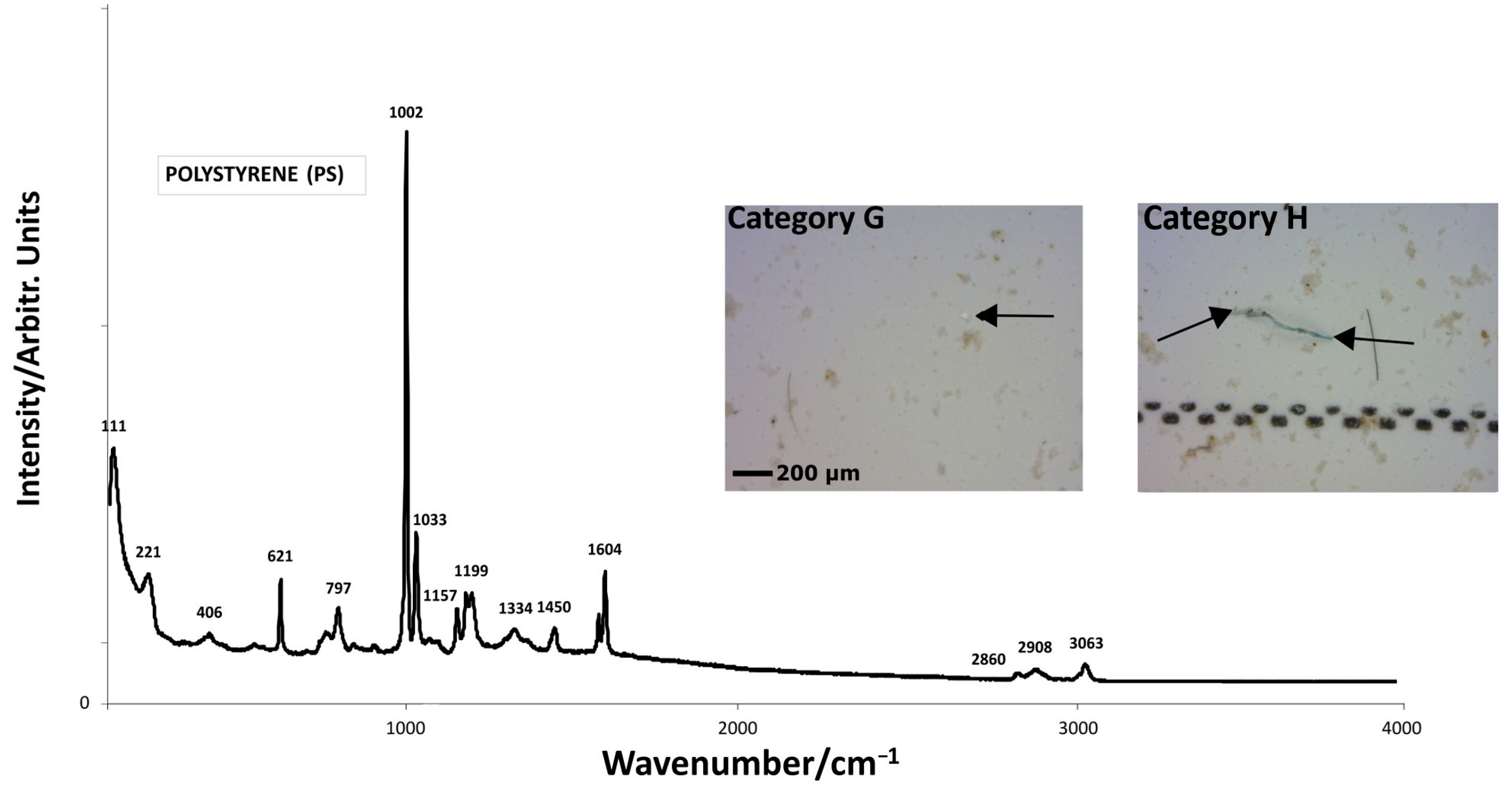
3.2. Raman Spectroscopy

Considering that most of the samples contained particles of each visual category, four randomly selected samples (three well samples and one borehole sample) covering most of the Erasinos catchment were subjected to μ-Raman analysis.
The 194 microplastics from each sample and category were analyzed using RS; RS analysis showed that each visual category was indicative of microplastics. In total, four different types of MPs were identified in the four samples based on their characteristic Raman peaks, namely, polyethylene (PE), polypropylene (PP), polystyrene (PS), and polyethylene terephthalate (PET) (Table 5, Figure 4, Figure 5, Figure 6 and Figure 7). In general, the peaks in the spectral range 2780–2980 cm−1 of the Raman spectra of MPs correspond to the stretching vibrations of CH/CH2/CH3 groups; in the spectral range 1580–1640 cm−1, to the aromatic bending vibrations, and in the spectral range 709–759 cm−1, to the symmetric stretching vibrations of CF2 [15,33]. In total, four different types of MPs polymers can be identified by their Raman peaks in these three spectral regions. In detail:
Polyethylene (PE) was identified in three samples (GW1, GW2, GW4), mainly by the two intense peaks at ~2850 and 2885 cm−1 corresponding to CH2 stretching vibrations. Moreover, the antisymmetric and symmetric stretching vibrations of C–C at ~1062 cm−1 and 1129 cm−1, respectively, and the bending vibrations of CH2 at 1296 and 1440 cm−1, were clearly visible in the Raman spectra of PE. The weak peak at ~2725 cm−1 is an overtone of wavenumbers in the range 1400–1495 cm−1 (–CH2 bonds). In the spectral region below 1000 cm−1, stretching and bending vibrations of C–C are expected, possibly together with CH2 twisting and rocking vibrations of methylene units in a Gauche relation. A typical spectrum of PE is shown in Figure 4a. In Figure 4b,c, in addition to the bands of PE (at ~1062, 1129, 1296, 1417, 1440, 1460, 2725, 2850, and 2885 cm−1), bands appear at ~483, 678, 746, 955, 1145, and 1530 cm−1. These bands are attributed to the blue pigment copper phthalocyanine (Pigment Blue 15, IRUG collection #ROD00126 [34]), which is often used to color plastics and is consistent with the blue color of these MPs. Polyethylene was identified in samples GW1, GW2, and GW4 (40% of the total Raman analyses) mainly in category A, followed by D, B, and E.
Figure 4. (ac) Raman spectra of polyethylene-type MPs, found in the studied samples. The black arrow on the inset shows the analyzed MP. In (b,c) additional peaks at ~682, 750, and 1532 cm−1 are assigned to the pigment copper phthalocyanine (Pigment Blue 15, IRUG collection #ROD00126 [34]).
Water 16 00843 g004
Isotactic polypropylene (iPP) was found in three samples (GW1, GW2, and GW3, 35%). It is characterized by intense peaks at 396 cm−1 attributed to CH2 wagging and CH bending, at ~809 cm−1 corresponding to the rocking vibrations of CH2 and stretching vibrations of C–C and C–CH3, at 841 cm−1 due to the rocking of CH2 and CH3 and the stretching of C–C and C–CH3, at 973 cm−1 assigned to CH3 rocking and C–C stretching, at 1153 cm−1 resulting by stretching vibrations of C–C and C–CH3, bending vibrations of CH, and rocking vibrations of CH, at 1330 cm−1 attributed to bending vibrations of CH, at 1360 cm−1 due to the symmetric bending of CH3 and CH bending, and at 1460 cm−1 due to the asymmetric bending of CH3 and CH2 bending (Figure 5b,c). The peaks of CH2 stretching vibrations between 2800 and 3000 cm−1 were relatively weak in some spectra, and a broad and strong band was also observed in the range of 2100–2200 cm−1. In Figure 5b,c, additional peaks at ~682, 750, and 1532 cm−1 are assigned to the pigment copper phthalocyanine (Pigment Blue 15, IRUG collection #ROD00126 [34]); this is consistent with the blue color of these two microplastic particles.
Figure 5. (ac) Raman spectra of polypropylene-type MPs, found in the studied samples. The black arrow on the inset shows the analyzed MP.
Water 16 00843 g005
Polyethylene terephthalate (PET) was identified in all samples studied (25%), mainly in category F, followed by D and G. The peak at approximately 1100 cm−1 corresponds to C–O and C–C stretching or C–O–C bending. A shoulder at about 1120 cm−1 indicates an amorphous phase. The peak at ~1615 cm−1 is due to the C-C ring of phenyl, and the peak at ~1730 cm−1 is assigned to the stretching vibrations of C=O. Between 2800 and 3000 cm−1, the peaks of CH2 stretching vibrations arise (Figure 6). The peak at 817 cm−1 in Figure 6b is attributed to C−H out-of-plane bending vibrations in para-xylene (p-xylene) [35,36].
Figure 6. (ac) Raman spectra of polyethylene terephthalate-type MPs, found in the studied samples. The black arrow on the inset shows the analyzed MP.
Water 16 00843 g006
Polystyrene (PS), identified only in sample GW1 (10%), provided intense Raman peaks at 1002 cm−1, corresponding to C–C symmetric stretching vibrations (Figure 7). Other characteristic PS bands were observed at ~621, 797, 1033, 1157, 1450, and 1604 cm−1, corresponding to the ν6b radial ring-stretching mode, ν1 symmetric ring-stretching mode, ν18a tangential C–H bending mode, ν15 mode, ν19b stretching or CH2 bending vibrations, and ν12 C–C stretching mode, respectively [37,38]. Overlapping bands at 3060 cm−1 appear due to the C–H bonds stretching on the benzene ring.
Figure 7. Raman spectra of polystyrene MPs, found in the studied samples. The black arrow on the inset shows the analyzed MP.
Water 16 00843 g007
Finally, some blue fibers analyzed yielded the Raman spectrum of the pigment indigo blue (250, 545, 599, 1310, 1228, 1575, and 1584 cm−1 [39]. Due to the high background of these spectra, it was not possible to identify the substrate of the pigment.
Raman spectroscopy on microparticles in the groundwater samples investigated also revealed the presence of inorganic mineral phases, mainly carbonates (calcite, dolomite) and quartz.
By combining the results of virtual sorting and Raman microspectroscopy, we found the following:
Polyethylene (PE) was found mainly in the form of dark and light blue fibers >150 μm long (visual categories A and B). A limited number of blue angular, irregular, and in a few cases acicular particles with a size of >30 μm (visual category D), and very rare red-to-orange particles and granules with a size of >25 μm, were also identified as PE.
Polypropylene (PP) was found mainly in the form of blue fibers >150 μm long (visual category A). Angular, irregular particles of a blue (visual category D) and whitish-gray (visual category Ε) color sized >25 μm were also identified as PP.
Polyethylene terephthalate (PET) was found mainly as irregular, angular-to-medium/semi-rounded particles and granules of a color ranging from pale yellow, beige, whitish, and white to gray and of a size of >20 μm (visual category F). A few angular, irregular particles of a blue color (visual category D) and a limited number of highly reflective angular, irregular particles in vertical reflected light (visual category G) were also identified as PET.
A very limited number of PS MPs were identified as highly reflective irregular, angular particles (visual category G) and blue–colored fibers characterized by a high heterogeneity in shape, texture, and thickness (visual category H).
Table 5. Identified polymer types in the studied samples based on their Raman peaks.
Polymer TypesPolymer FormulaRaman Peaks (cm−1)SampleVisual Categories
PEWater 16 00843 i001
(C2H4)n
1062sasC–C) [40,41,42]
~1129ssC–C) [40,41,42]
1296s (τCH2) [40,41,42]
~1417m (ωCH2) [42]
~1440s (δCH2) [40,41]
1512w (δCH2) [40,41]
~2850 (νsCH2) [43,44]
~2884sasCH2) [43,44]
GW1, GW2, GW4A,B,D,E
PPWater 16 00843 i002
(C3H6)n
396s (ωCH2,δCH) [45,46]
809vs (ρCH2, vCC, vC–CH3 [42,45,46]
841s (pCH2, vCCb, vC–CH3, pCH3) [45,46]
973m (ρCH3 + vC–C chain) [45,46]
1153s (vCCb, vC–CH3, δCH, pCH3) [45,46]
~1330s (δCH) [45,46]
~1460s (δCH3) [45,46]
~2842m(νCH2) [43,44]
2860m(νCH2) [43,44]
~2885ssCH3) [43,44]
2954-2963maCH3) [43,44]
GW1, GW2, GW3A,C,D,F
PSWater 16 00843 i003
(C8H8)n
621s (νC–C) [37,38]
797m (νsC–C) [37,38]
1002s (νC–C) [45]
1033 (δC–H) [37]
1157w (ν15 mode) [37]
1450w [ν19b or δ(CH2)] [37]
1604msC–C) [37]
2860wsCH2) [42]
2908wasCH2) [42]
3063w (νC–H) [42]
GW1G,H
PETWater 16 00843 i004
(C10H8O4)n
860s (ρCH2)
1097m (νC–O, νC–C, δC–O–C) [47]
1612-1617s (C–C ring of phenyl) [43,47]
1726-1730s (νC=O) [47]
2850w,m (νCH2) [43,47]
2883w,m (νCH2) [43,47]
3081w (C–H of phenyl) [43,47]
GW1, GW2, GW3, GW4D,F,G

4. Discussion

In view of the above, visual presorting, while a very time-consuming method, does not provide an unambiguous identification of the type of MPs in a sample; the latter is only possible with the use of a microspectroscopy method such as RS. However, visual presorting is faster in quantifying the total number of MPs in a sample. Future challenges in this field include the use of Raman hyperspectral mapping on filters aiming not only the identification but also the quantification of MPs, and/or the in situ identification of MPs with portable Raman microspectrometers.
Polyethylene and PP were the most abundant MPs in the samples studied. This is consistent with the fact that these two plastic polymers are the most commonly produced in the world and are therefore frequently found in relevant studies, especially in the marine environment (e.g., [48]).
Although one might attribute the abundance of blue MPs in the studied samples to possibly biased visual presorting, this could be explained by the faster photoaging of blue plastics compared to red or yellow plastics. As stated by Zhao et al. [6] in the visible light region, red or yellow pigments with longer wavelengths may absorb short-wave light with higher energy, while blue pigments absorb long-wavelength light with lower energy. The corresponding light energy transmitted to the blue plastic is consequently higher than that transmitted to red or yellow plastics, which makes the photoaging more intense. Because blue plastics cannot absorb UV light effectively, they age faster when exposed to sunlight, and higher levels of bluish microplastics are often found in the environment, especially in the smallest sizes [49].
Copper phthalocyanine (Pigment Blue 15), a common blue pigment used for dyeing plastics (e.g., [50]), was identified in both PP and PE MPs. In general, the MPs in the form of blue-colored fibers mainly correspond to either PP or PE and, less frequently, PS. Overall, RS confirmed that all identified particles were indeed MPs. Even though MPs are visually similar and belong to the same optical categories, RS has shown that they can differ in nature. Nevertheless, there is a trend that separates PP and PE, in one visual group (A, B, D), from PS and PET, which are part of another visual group (G, H, E). This trend needs further research.
Samples SW2 and SW4 are the only samples that have MPs from all eight categories, while GW4 has the least number of MPs and fewer categories. This was to be expected, as samples SW2 and SW4 were collected from surface water which is (a) generally more contaminated due to its proximity to human activities that generate MPs and (b) exposed to the atmosphere, so that MPs can also be enriched by air. Furthermore, it is very important to mention that they were collected at the estuary of Erasinos (SW4) and at the sea, where the river flows in and has accumulated MPs from the entire catchment area. This is also justified by the fact that more MPs were detected in samples SW1, GW5, SW2, SW3, SW4, SW5, GW6, GW7, GW8, GW9, GW10, and GW11, collected downstream, than in samples GW1, GW2, GW3, and GW4, which were collected further upstream of the catchment. Comparing the results in Figure 3, it can be assumed that surface water is generally more susceptible to MP contamination than groundwater, as on average, more MP particles/L of water samples were detected. On the other hand, it is interesting to note that MPs, and in particular PET and PE, were detected in the sample from the water borehole, suggesting that MPs can migrate to greater depths through water infiltration. Another alternative scenario for tracing MPs at greater water depths would be the possibility of waste injection through other boreholes.
The role of inorganic mineral phases such as carbonates and quartz in connection with microplastics needs further investigation in the future. Column experiments have shown that the presence of iron and manganese oxides, as well as calcite, not only changes the transport behavior of plastics, but can also shield plastics from UV light (e.g., [51,52]). In this context, it was investigated whether the groundwater tends to dissolve or precipitate the minerals calcite, dolomite, and quartz in particular. The positive SI value of these minerals indicates that the water is oversaturated in relation to the solution, which leads to the precipitation of these minerals. These mineral phases were also identified by Raman analyses, which confirmed their precipitation. Saturation-induced precipitation leads to the formation of small crystals on the surface of MPs.
A major challenge for researchers is the mechanism of how microplastics migrate through the vadose zone into the saturated zone and how they contaminate groundwater. The hydrogeological conditions of a region appear to play a key role in the transport of microplastics via different pathways. The most important hydrogeological factors that have recently been suggested to influence the distribution and migration of microplastics in groundwater are as follows [53,54,55]: (a) the permeability and porosity of an aquifer, which favor the size of microplastics that can migrate into groundwater, (b) the recharge of the aquifer by surface runoff, (c) the structure of the vadose zone, (d) the seasonal periods of recharge, (e) the hydraulic conductivity of an aquifer, (f) the water–soil interaction, (g) the groundwater velocity, (h) the lateral hydraulic connection between aquifers or the intrusion of seawater, and (i) the water depth. Another important factor for the migration of microplastics into groundwater is the type of sources, i.e, diffuse linear sources (torrents, rivers, streams) or point sources (spills, etc.), as well as the land cover of an area [56]. However, the extent to which these individual factors influence the migration of MPs and their interactions is an open field for future research.
The physico-chemical properties of the analyzed water samples (surface and groundwater) indicate the decisive role of anthropogenic activities in the area. According to Wang et al. [57], the pH of water could theoretically influence the sorption of ionic chemicals by MPs. The high values of E.C., Ca2+, Mg2+, Cl, and Na+ indicate the intrusion of seawater into the coastal area of the Erasinos basin due to the overexploitation of aquifers for irrigation. Agricultural activities are also a potential source of microplastics in surface and groundwater, mainly due to plastic bottles and the plastic in greenhouses. Agricultural activities in the study area were confirmed by the high NO3 and PO43- concentrations depicted in Table 2. In addition, major anions and cations are abundant in the groundwater environment [19]. It is hypothesized that the increased concentrations of Ca2+ forms increase the number of adsorption sites and enhance the adsorption of microplastics in the media. In contrast, it is assumed that the influence of increased concentrations of HCO3 and SO42−, in the water solution reduces the adsorption of MPs on the surface of the aquifers [19]. Monitoring the chemical properties of groundwater, in conjunction with the quantification and identification of MPs, will provide sufficient results when considering the correlation between chemical parameters and the presence of MPs. The latter may facilitate tracing the influence of different sources of MPs among the samples. This study can contribute to future databases that may correlate the presence of certain MPs with specific sources and environments supported by the geochemical analyses.
In the Erasinos basin, groundwater recharge from seepage of the Erasinos River and other surface runoff (torrents, rivers, streams) could potentially enhance the migration of MPs to the saturated zone. As seawater infiltrates into the nearshore part of the basin, there is a hydraulic connection between the aquifer system and the sea, which could represent an additional source of MPs.
This study is the first systematic work on MPs in groundwater in Attica, Greece, and one of the few worldwide [58,59,60] that have recently investigated the presence and transport of microplastics in groundwater. The results indicate that the investigation of microplastics in other aquifers needs to be expanded in order to monitor the extent of contamination and trace the sources where possible. As groundwater is in many cases not only used for irrigation but also as drinking water, it is of great importance and relevant for public health to investigate the occurrence of microplastics more systematically.
The concentrations of MPs are not stable and standardized in a region and vary due to the geomorphological characteristics, hydrogeological conditions, atmospheric conditions, and land use of each area, since they define the MPs sources. For example, the amount of MPs in shallow aquifers close to industrial and agricultural activities can be as high as 6832 MP particles/L [61]. In contrast, an average of 6.4 particles/L [53] was observed in karstic aquifers with low anthropogenic activities. In our study area, the high amount of microplastics (3399 particles/ per 16 Liters) is related to the intensive anthropogenic activities (agricultural, industrial, and urban) in this area, combined with the shallow aquifer.

5. Conclusions

In this work, we have investigated and documented for the first time the occurrence of MPs in groundwater in shallow and deep aquifers in Attica, Greece. Based on our results, the following conclusions can be drawn:
The characterization of MPs by Raman microspectroscopy revealed the presence of the following:
a.
PE and PP in the form of fibers and fragments;
b.
PET as angular irregular particles;
c.
PS as reflective irregular angular particles and blue-colored fibers.
Microplastics are more prevalent in shallow aquifers, as expected, reaching up to 513 MPs/L. In the deeper aquifers (water table ~70 m), the abundance of MPs is lower (up to 16 MPs/L); however, this is no less significant, as it may indicate that MPs are able to migrate to greater depths through water infiltration.
The types of MPs appear to vary due to different land use and the vulnerability of groundwater systems. A high amount of microplastics (3399 particles/ per 16 Liters) was found where intensive anthropogenic activities (agricultural, industrial, and urban) take place.
The mechanism of MPs admission into the deep (water table ~70 m) aquifer needs further investigation. Seawater intrusion, which is reflected in the qualitative characteristics of groundwater, could potentially be a source of microplastics. The extent at which seawater MP contamination interacts with other potential sources such as agricultural activities requires further in-depth geochemical investigations, to document the correlation between MPs and key chemical parameters.
This study can contribute to future databases that, supported by geochemical analyses, will link the presence of MPs to specific sources and environments.

Author Contributions

Conceptualization, M.P., E.V. and I.P.; methodology, M.P., E.V. and I.P.; resources: P.M., E.V., C.S., I.P. and G.S.; investigation, all; data curation, P.M., V.S. and C.S.; writing—original draft preparation, M.P. and V.S.; writing—review and editing, all; supervision, M.P., E.V. and I.P. All authors have read and agreed to the published version of the manuscript.

Funding

This research received no external funding.

Data Availability Statement

Data are contained within the article.

Conflicts of Interest

The authors declare no conflicts of interest.

References

  1. Cowger, W.; Gray, A.; Christiansen, S.H.; DeFrond, H.; Deshpande, A.D.; Hemabessiere, L.; Lee, E.; Mill, L.; Munno, K.; Ossmann, B.E.; et al. Critical Review of Processing and Classification Techniques for Images and Spectra in Microplastic Research. Appl. Spectrosc. 2020, 74, 989–1010. [Google Scholar] [CrossRef] [PubMed]
  2. Silva, A.B.; Bastos, A.S.; Justino, C.I.L.; da Costa, J.P.; Duarte, A.C.; Rocha-Santos, T.A.P. Microplastics in the Environment: Challenges in Analytical Chemistry—A Review. Anal. Chim. Acta 2018, 1017, 1–19. [Google Scholar] [CrossRef] [PubMed]
  3. Arthur, C.; Baker, J.E.; Bamford, H.A. NOAA Technical Memorandum NOS-OR&R-30. In Proceedings of the International Research Workshop on the Occurrence, Effects, and Fate of Microplastic Marine Debris, University of Washington Tacoma, Tacoma, WA, USA, 9–11 September 2008. [Google Scholar]
  4. Ziani, K.; Ioniță-Mîndrican, C.-B.; Mititelu, M.; Neacșu, S.M.; Negrei, C.; Moroșan, E.; Drăgănescu, D.; Preda, O.-T. Microplastics: A Real Global Threat for Environment and Food Safety: A State of the Art Review. Nutrients 2023, 15, 617. [Google Scholar] [CrossRef]
  5. An, L.; Liu, Q.; Deng, Y.; Wu, W.; Gao, Y.; Ling, W. Sources of Microplastic in the Environment. In Microplastics in Terrestrial Environments: Emerging Contaminants and Major Challenges; He, D., Luo, Y., Eds.; The Handbook of Environmental Chemistry; Springer International Publishing: Cham, Switzerland, 2020; pp. 143–159. [Google Scholar] [CrossRef]
  6. Zhao, X.; Wang, J.; Yee Leung, K.M.; Wu, F. Color: An Important but Overlooked Factor for Plastic Photoaging and Microplastic Formation. Environ. Sci. Technol. 2022, 56, 9161–9163. [Google Scholar] [CrossRef]
  7. Suaria, G.; Avio, C.G.; Mineo, A.; Lattin, G.L.; Magaldi, M.G.; Belmonte, G.; Moore, C.J.; Regoli, F.; Aliani, S. The Mediterranean Plastic Soup: Synthetic Polymers in Mediterranean Surface Waters. Sci. Rep. 2016, 6, 37551. [Google Scholar] [CrossRef]
  8. Isobe, A.; Iwasaki, S.; Uchida, K.; Tokai, T. Abundance of Non-Conservative Microplastics in the Upper Ocean from 1957 to 2066. Nat. Commun. 2019, 10, 417. [Google Scholar] [CrossRef]
  9. Peeken, I.; Primpke, S.; Beyer, B.; Gütermann, J.; Katlein, C.; Krumpen, T.; Bergmann, M.; Hehemann, L.; Gerdts, G. Arctic Sea Ice Is an Important Temporal Sink and Means of Transport for Microplastic. Nat. Commun. 2018, 9, 1505. [Google Scholar] [CrossRef]
  10. González-Pleiter, M.; Velázquez, D.; Edo, C.; Carretero, O.; Gago, J.; Baron-Sola, Á.; Hernández, L.E.; Yousef, I.; Quesada, A.; Leganés, F.; et al. Fibers Spreading Worldwide: Microplastics and Other Anthropogenic Litter in an Arctic Freshwater Lake. Sci. Total Environ. 2020, 722, 137904. [Google Scholar] [CrossRef]
  11. Nguyen, N.B.; Kim, M.-K.; Le, Q.T.; Ngo, D.N.; Zoh, K.-D.; Joo, S.-W. Spectroscopic Analysis of Microplastic Contaminants in an Urban Wastewater Treatment Plant from Seoul, South Korea. Chemosphere 2021, 263, 127812. [Google Scholar] [CrossRef]
  12. Hidalgo-Ruz, V.; Gutow, L.; Thompson, R.C.; Thiel, M. Microplastics in the Marine Environment: A Review of the Methods Used for Identification and Quantification. Environ. Sci. Technol. 2012, 46, 3060–3075. [Google Scholar] [CrossRef] [PubMed]
  13. Shan, J.; Zhao, J.; Liu, L.; Zhang, Y.; Wang, X.; Wu, F. A Novel Way to Rapidly Monitor Microplastics in Soil by Hyperspectral Imaging Technology and Chemometrics. Environ. Pollut. 2018, 238, 121–129. [Google Scholar] [CrossRef] [PubMed]
  14. Fu, W.; Min, J.; Jiang, W.; Li, Y.; Zhang, W. Separation, Characterization and Identification of Microplastics and Nanoplastics in the Environment. Sci. Total Environ. 2020, 721, 137561. [Google Scholar] [CrossRef] [PubMed]
  15. Käppler, A.; Fischer, D.; Oberbeckmann, S.; Schernewski, G.; Labrenz, M.; Eichhorn, K.-J.; Voit, B. Analysis of Environmental Microplastics by Vibrational Microspectroscopy: FTIR, Raman or Both? Anal. Bioanal. Chem. 2016, 408, 8377–8391. [Google Scholar] [CrossRef]
  16. Käppler, A.; Windrich, F.; Löder, M.G.J.; Malanin, M.; Fischer, D.; Labrenz, M.; Eichhorn, K.-J.; Voit, B. Identification of Microplastics by FTIR and Raman Microscopy: A Novel Silicon Filter Substrate Opens the Important Spectral Range below 1300 Cm−1 for FTIR Transmission Measurements. Anal. Bioanal. Chem. 2015, 407, 6791–6801. [Google Scholar] [CrossRef]
  17. Lee, J.-Y.; Cha, J.; Ha, K.; Viaroli, S. Microplastic Pollution in Groundwater: A Systematic Review. Environ. Pollut. Bioavailab. 2024, 36, 2299545. [Google Scholar] [CrossRef]
  18. Ma, H.; Chao, L.; Wan, H.; Zhu, Q. Microplastic Pollution in Water Systems: Characteristics and Control Methods. Diversity 2024, 16, 70. [Google Scholar] [CrossRef]
  19. Li, S.; Yang, M.; Wang, H.; Jiang, Y. Adsorption of Microplastics on Aquifer Media: Effects of the Action Time, Initial Concentration, Ionic Strength, Ionic Types and Dissolved Organic Matter. Environ. Pollut. 2022, 308, 119482. [Google Scholar] [CrossRef] [PubMed]
  20. Ioakeimidis, C.; Fotopoulou, K.N.; Karapanagioti, H.K.; Geraga, M.; Zeri, C.; Papathanassiou, E.; Galgani, F.; Papatheodorou, G. The Degradation Potential of PET Bottles in the Marine Environment: An ATR-FTIR Based Approach. Sci. Rep. 2016, 6, 23501. [Google Scholar] [CrossRef]
  21. Tziourrou, P.; Megalovasilis, P.; Tsounia, M.; Karapanagioti, H.K. Characteristics of Microplastics on Two Beaches Affected by Different Land Uses in Salamina Island in Saronikos Gulf, East Mediterranean. Mar. Pollut. Bull. 2019, 149, 110531. [Google Scholar] [CrossRef]
  22. Tsangaris, C.; Digka, N.; Valente, T.; Aguilar, A.; Borrell, A.; de Lucia, G.A.; Gambaiani, D.; Garcia-Garin, O.; Kaberi, H.; Martin, J.; et al. Using Boops Boops (Osteichthyes) to Assess Microplastic Ingestion in the Mediterranean Sea. Mar. Pollut. Bull. 2020, 158, 111397. [Google Scholar] [CrossRef]
  23. Karkanorachaki, K.; Kiparissis, S.; Kalogerakis, G.C.; Yiantzi, E.; Psillakis, E.; Kalogerakis, N. Plastic Pellets, Meso- and Microplastics on the Coastline of Northern Crete: Distribution and Organic Pollution. Mar. Pollut. Bull. 2018, 133, 578–589. [Google Scholar] [CrossRef] [PubMed]
  24. Jacobshagen, V. Geologie von Griechenland. Available online: https://www.schweizerbart.de/publications/detail/isbn/9783443110192/Geologie_von_Griechenland (accessed on 27 January 2024).
  25. Katsikatsos, G. Geology of Greece; University of Patras: Patras, Greece, 1992. [Google Scholar]
  26. Champidi, P.; Stamatis, G.; Zagana, E. Groundwater Quality Assessment and Geogenic and Anthropogenic Effect Estimation in Erasinos Basin (E. Attica). Eur. Water 2011, 33, 11–27. [Google Scholar]
  27. Stamatis, G.; Lambrakis, N.; Alexakis, D.; Zagana, E. Groundwater Quality in Mesogea Basin in Eastern Attica (Greece). Hydrol. Process. 2006, 20, 2803–2818. [Google Scholar] [CrossRef]
  28. Latsoudas, X. Geological Map “Koropi-Plaka”, Scale 1:50.000; Institute of Geology and Mineral Exploration: Athens, Greece, 2003. [Google Scholar]
  29. Koelmans, A.A.; Mohamed Nor, N.H.; Hermsen, E.; Kooi, M.; Mintenig, S.M.; De France, J. Microplastics in Freshwaters and Drinking Water: Critical Review and Assessment of Data Quality. Water Res. 2019, 155, 410–422. [Google Scholar] [CrossRef]
  30. Kutralam-Muniasamy, G.; Shruti, V.C.; Pérez-Guevara, F.; Roy, P.D.; Elizalde-Martínez, I. Common Laboratory Reagents: Are They a Double-Edged Sword in Microplastics Research? Sci. Total Environ. 2023, 875, 162610. [Google Scholar] [CrossRef] [PubMed]
  31. Merkel, B.; Friedrich, B. Groundwater Geochemistry: A Practical Guide to Modeling of Natural and Contaminated Aquatic Systems; Nordstorm, D.K., Ed.; Springer: Berlin/Heidelberg, Germany, 2005. [Google Scholar] [CrossRef]
  32. Shruti, V.C.; Kutralam-Muniasamy, G. Blanks and Bias in Microplastic Research: Implications for Future Quality Assurance. Trends Environ. Anal. Chem. 2023, 38, e00203. [Google Scholar] [CrossRef]
  33. Jin, N.; Song, Y.; Ma, R.; Li, J.; Li, G.; Zhang, D. Characterization and Identification of Microplastics Using Raman Spectroscopy Coupled with Multivariate Analysis. Anal. Chim. Acta 2022, 1197, 339519. [Google Scholar] [CrossRef]
  34. Scherrer, N.C.; Stefan, Z.; Francoise, D.; Annette, F.; Renate, K. Synthetic Organic Pigments of the 20th and 21st Century Relevant to Artist’s Paints: Raman Spectra Reference Collection. Spectrochim. Acta Part A Mol. Biomol. Spectrosc. 2009, 73, 505–524. [Google Scholar] [CrossRef]
  35. Vedad, J.; Reilly, L.; Desamero, R.Z.B.; Mojica, E.-R.E. Quantitative Analysis of Xylene Mixtures Using a Handheld Raman Spectrometer. In Raman Spectroscopy in the Undergraduate Curriculum; ACS Symposium Series; American Chemical Society: Washington, DC, USA, 2018; Volume 1305, pp. 129–152. [Google Scholar] [CrossRef]
  36. Lapa, H.M.; Martins, L.M.D.R.S. P-Xylene Oxidation to Terephthalic Acid: New Trends. Molecules 2023, 28, 1922. [Google Scholar] [CrossRef]
  37. Zhou, X.-X.; Liu, R.; Hao, L.-T.; Liu, J.-F. Identification of Polystyrene Nanoplastics Using Surface Enhanced Raman Spectroscopy. Talanta 2021, 221, 121552. [Google Scholar] [CrossRef]
  38. Kellar, E.J.C.; Galiotis, C.; Andrews, E.H. Raman Vibrational Studies of Syndiotactic Polystyrene. 1. Assignments in a Conformational/Crystallinity Sensitive Spectral Region. Macromolecules 1996, 29, 3515–3520. [Google Scholar] [CrossRef]
  39. Caggiani, M.C.; Cosentino, A.; Mangone, A. Pigments Checker Version 3.0, a Handy Set for Conservation Scientists: A Free Online Raman Spectra Database. Microchem. J. 2016, 129, 123–132. [Google Scholar] [CrossRef]
  40. Gall, M.J.; Hendra, P.J.; Peacock, C.J.; Cudby, M.E.A.; Willis, H.A. Laser-Raman Spectrum of Polyethylene: Part 1. Structure and Analysis of the Polymer. Polymer 1972, 13, 104–108. [Google Scholar] [CrossRef]
  41. Fischer, J.; Wallner, G.M.; Pieber, A. Spectroscopical Investigation of Ski Base Materials. Macromol. Symp. 2008, 265, 28–36. [Google Scholar] [CrossRef]
  42. Nava, V.; Frezzotti, M.L.; Leoni, B. Raman Spectroscopy for the Analysis of Microplastics in Aquatic Systems. Appl. Spectrosc. 2021, 75, 1341–1357. [Google Scholar] [CrossRef] [PubMed]
  43. Dong, M.; Zhang, Q.; Xing, X.; Chen, W.; She, Z.; Luo, Z. Raman Spectra and Surface Changes of Microplastics Weathered under Natural Environments. Sci. Total Environ. 2020, 739, 139990. [Google Scholar] [CrossRef] [PubMed]
  44. Kniggendorf, A.-K.; Wetzel, C.; Roth, B. Microplastics Detection in Streaming Tap Water with Raman Spectroscopy. Sensors 2019, 19, 1839. [Google Scholar] [CrossRef] [PubMed]
  45. De Baez, M.A.; Hendra, P.J.; Judkins, M. The Raman spectra of oriented isotactic polypropylene. Spectrochim. Acta Part A Mol. Biomol. Spectrosc. 1995, 51, 2117–2124. [Google Scholar] [CrossRef]
  46. Andreassen, E. Infrared and Raman Spectroscopy of Polypropylene. In Polypropylene; Karger-Kocsis, J., Ed.; Polymer Science and Technology Series; Springer: Dordrecht, The Netherlands, 1999; Volume 2, pp. 320–328. [Google Scholar] [CrossRef]
  47. Ciera, L.; Beladjal, L.; Almeras, X.; Gheysens, T.; Van Landuyt, L.; Mertens, J.; Nierstrasz, V.; Van Langenhove, L. Morphological and Material Properties of Polyethyleneterephthalate (PET) Fibres with Spores Incorporated. Fibres Text. East. Eur. 2014, 22, 29–36. [Google Scholar]
  48. Prata, J.C.; da Costa, J.P.; Duarte, A.C.; Rocha-Santos, T. Methods for Sampling and Detection of Microplastics in Water and Sediment: A Critical Review. TrAC Trends Anal. Chem. 2019, 110, 150–159. [Google Scholar] [CrossRef]
  49. Martí, E.; Martin, C.; Galli, M.; Echevarría, F.; Duarte, C.M.; Cózar, A. The Colors of the Ocean Plastics. Environ. Sci. Technol. 2020, 54, 6594–6601. [Google Scholar] [CrossRef]
  50. Gregory, P. Industrial Applications of Phthalocyanines. J. Porphyr. Phthalocyanines 2000, 4, 432–437. [Google Scholar] [CrossRef]
  51. Leiser, R.; Jongsma, R.; Bakenhus, I.; Möckel, R.; Philipp, B.; Neu, T.R.; Wendt-Potthoff, K. Interaction of Cyanobacteria with Calcium Facilitates the Sedimentation of Microplastics in a Eutrophic Reservoir. Water Res. 2021, 189, 116582. [Google Scholar] [CrossRef] [PubMed]
  52. Dodhia, M.S.; Rogers, K.L.; Fernández-Juárez, V.; Carreres-Calabuig, J.A.; Löscher, C.R.; Tisserand, A.A.; Keulen, N.; Riemann, L.; Shashoua, Y.; Posth, N.R. Microbe-Mineral Interactions in the Plastisphere: Coastal Biogeochemistry and Consequences for Degradation of Plastics. Front. Mar. Sci. 2023, 10, 1134815. [Google Scholar] [CrossRef]
  53. Panno, S.V.; Kelly, W.R.; Scott, J.; Zheng, W.; McNeish, R.E.; Holm, N.; Hoellein, T.J.; Baranski, E.L. Microplastic Contamination in Karst Groundwater Systems. Groundwater 2019, 57, 189–196. [Google Scholar] [CrossRef] [PubMed]
  54. Severini, E.; Ducci, L.; Sutti, A.; Robottom, S.; Sutti, S.; Celico, F. River–Groundwater Interaction and Recharge Effects on Microplastics Contamination of Groundwater in Confined Alluvial Aquifers. Water 2022, 14, 1913. [Google Scholar] [CrossRef]
  55. Gong, X.; Tian, L.; Wang, P.; Wang, Z.; Zeng, L.; Hu, J. Microplastic Pollution in the Groundwater under a Bedrock Island in the South China Sea. Environ. Res. 2023, 239, 117277. [Google Scholar] [CrossRef] [PubMed]
  56. Ye, S.; Pei, D. Relationships between Microplastic Pollution and Land Use in the Chongqing Section of the Yangtze River. Front. Ecol. Evol. 2023, 11, 1202562. [Google Scholar] [CrossRef]
  57. Wang, F.; Shih, K.M.; Li, X.Y. The Partition Behavior of Perfluorooctanesulfonate (PFOS) and Perfluorooctanesulfonamide (FOSA) on Microplastics. Chemosphere 2015, 119, 841–847. [Google Scholar] [CrossRef]
  58. Shockley, D.J.; Lapworth, D.J. Microplastics in Groundwater: A Literature Review. Available online: https://nora.nerc.ac.uk/id/eprint/532669/ (accessed on 27 January 2024).
  59. Alvarado-Zambrano, D.; Rivera-Hernández, J.R.; Green-Ruiz, C. First Insight into Microplastic Groundwater Pollution in Latin America: The Case of a Coastal Aquifer in Northwest Mexico. Environ. Sci. Pollut. Res. 2023, 30, 73600–73611. [Google Scholar] [CrossRef]
  60. Sangkham, S.; Aminul Islam, M.d.; Adhikari, S.; Kumar, R.; Sharma, P.; Sakunkoo, P.; Bhattacharya, P.; Tiwari, A. Evidence of Microplastics in Groundwater: A Growing Risk for Human Health. Groundw. Sustain. Dev. 2023, 23, 100981. [Google Scholar] [CrossRef]
  61. Mu, H.; Wang, Y.; Zhang, H.; Guo, F.; Li, A.; Zhang, S.; Liu, S.; Liu, T. High Abundance of Microplastics in Groundwater in Jiaodong Peninsula, China. Sci. Total Environ. 2022, 839, 156318. [Google Scholar] [CrossRef] [PubMed]
Figure 2. Sampling sites in the Erasinos basin (Google Earth).
Water 16 00843 g002
Figure 3. (a) MPs/L/Surface water, (b) MPs/L/Groundwater.
Water 16 00843 g003
Table 1. Sampling sites.
Sample IDX LongitudeY LatitudeElevation (m.a.s.l.) *Notes
GW123°57′57.77″ E37°54′53.56″ N25 mWell—phreatic water table
GW223°57′43.44″ E37°54′50.45″ N33 mWell—phreatic water table
GW323°57′27.13″ E37°54′58.95″ N41 mWell—phreatic water table
GW423°52′59.76″ E37°54′53.20″ N103 mBorehole
SW123°59′29.80″ E37°55′33.56″ N10 mSurface water
GW523°59′38.50″ E37°55′17.50″ N9.5 mWell—phreatic water table
SW224°0′37.90″ E37°55′24.90″ N0 mSurface water—river mouth to the sea
SW324°0′0.85″ E37°55′29.64″ N8.5 mSurface water
SW424°0′3.50″ E37°55′29.85″ N0 mSurface water
SW523°58′33.4″ E37°55′7.40″ N19.5 mSurface water
GW623°58′32.55″ E37°55′5.16″ N19.8 mWell—phreatic water table
GW723°58′55.15″ E37°55′10.10″ N15.2 mWell—phreatic water table
GW823°58′55.11″ E37°55′22.59″ N12 mWell—phreatic water table
GW923°58′40.60″ E37°55′17.65″ N14 mWell—phreatic water table
GW1023°58′59.85″ E37°55′31.39″ N13.5 mWell—phreatic water table
GW1123°59′10.14″ E37°55′25.90″ N5.2 mWell—phreatic water table
Note: * m.a.s.l.: meters above sea level.
Table 2. Analyzed physical and chemical parameters of the investigated water samples in the Erasinos basin.
Sample IDpHTDSE.C.TempNa+K+Ca2+Mg2+ClHCO3NO3SiSO42−PO43−
mg/LµS/cm°Cmg/Lmg/Lmg/Lmg/Lmg/Lmg/Lmg/Lmg/Lmg/Lmg/L
SW17.4112617322199.3413639.4212.836631.710.71200.034
GW57.41807278022.63463.4208.874.2531.9317.272.264700.14
SW28.135,75055,0002010,300420435.21393.612,198.6170.8110.826400.055
SW37.81251192522206.65147.281.4425.5396.531.210.3162.50.145
SW47.811,44017,6002120870227.2506.66241.1549228.1195.50.13
SW57.7965148524.893.33.2116.843.7248.2329.436.19.843.80.069
GW67.41043160522.595.14142.447.7283.7347.740.510.51150.11
GW77.310401600221013.8123.269.1319.242716.78.972.50.07
GW87.9917141021.586.66.412039.3248.2384.312.39.517.50.935
GW97.11339206021.21143.6174.457.5372.336661.213.11250.14
GW106.914112170241222.2209.653.2407.8396.5489.987.50.07
GW117.589713802591.64.2123.266.7319.2372.136.58500.155
Table 3. Calculated saturation indices of the investigated water samples in the Erasinos basin.
Sample IDSI (Calcite)SI (Dolomite)SI (Quartz)
SW10.450.660.62
GW50.490.840.35
SW20.712.25−0.42
SW30.871.80.59
SW40.942.550.52
SW50.71.320.52
GW60.460.770.59
GW70.390.850.53
GW80.931.680.56
GW90.190.20.71
GW100.130.010.55
GW110.61.280.44
Table 4. Number of MPs particles/L per category identified in the investigated water samples in the Erasinos basin.
Category/Samples No of MPs Particles/LABCDEFGHTotal
SW1 (MPs particles/L)26724289040170
GW5 (MPs particles/L)1143101458026513
SW2 (MPs particles/L)166773347116403
SW3 (MPs particles/L)142270166115207
SW4 (MPs particles/L)277744123031372485
SW5 (MPs particles/L)3038195016126
GW6 (MPs particles/L)1754160220018280
GW7 (MPs particles/L)82270291857
GW8 (MPs particles/L)121153229013264
GW9 (MPs particles/L)1305820362221431
GW10 (MPs particles/L)9228377011112
GW11 (MPs particles/L)11115212809157
GW1 (MPs particles/L)171023314967
GW2 (MPs particles/L)180362360570
GW3 (MPs particles/L)10020370141
GW4 (MPs particles/L)4000056116
Total per category2073842139522612282813399
Disclaimer/Publisher’s Note: The statements, opinions and data contained in all publications are solely those of the individual author(s) and contributor(s) and not of MDPI and/or the editor(s). MDPI and/or the editor(s) disclaim responsibility for any injury to people or property resulting from any ideas, methods, instructions or products referred to in the content.

