
Fractal Characteristics of Water Outflows on the Soil Surface after a Pipe Failure


Department of Water Supply and Wastewater Disposal, Faculty of Environmental Engineering, Lublin University of Technology, Nadbystrzycka 40 B, 20-618 Lublin, Poland
*
Author to whom correspondence should be addressed.
Water 2024, 16(9), 1222; https://0-doi-org.brum.beds.ac.uk/10.3390/w16091222
Submission received: 20 March 2024
/
Revised: 11 April 2024
/
Accepted: 22 April 2024
/
Published: 25 April 2024
Abstract
:Water pipe failures result in real water losses in the form of water outflowing into the porous medium, such as the surrounding soil. Such an outflow may result in the creation of suffosion holes. The appropriate management of the water supply network may contribute to reducing the number of failures, but due to their random nature, it is not possible to completely eliminate them. Therefore, alternative solutions are being sought to reduce the effects of the failures. This article presents a fragment of the results from a broader scope of the research, which attempted to determine the outflow zone in relation to the fractal characteristics of water outflows. The research included the analysis of the actual geometric structures created by the water outflows, which were simplified into linear structures using isometric transformations. The structures were analyzed in terms of the parameters characterizing them, including their fractal dimensions. As a result, it was found that there was no relationship between the analyzed fractal parameters and the leakage area or hydraulic pressure in the water pipe. However, the influence of the number of points forming each linear structure on the analyzed parameters was shown. This allowed for the determination of further research aimed at estimating the size of the water outflow zone after the unsealing of an underground water supply pipe.
1. Introduction
The outflow of a liquid from a pressure pipe into a porous medium is a common phenomenon. It may occur during the failure of underground systems transporting liquids, for example, water supply networks. Owing to the efficient management of the water supply system and making of appropriate decisions and operational activities, the number of failures can be reduced, but they cannot be completely eliminated. The main reason that failures in water supply networks are inevitable is that they are very often random. Unwanted outflows from water pipes not only cause water loss but may also pose a threat to the safety of people and property. The cause of the threat is the possibility of water washing out particles from the soil matrix during a buried pipe failure, which may lead to the formation of empty spaces under the soil surface and the creation of land depressions (suffosion phenomenon). The accidents resulting from suffosion in urbanized areas are reported relatively often all over the world.
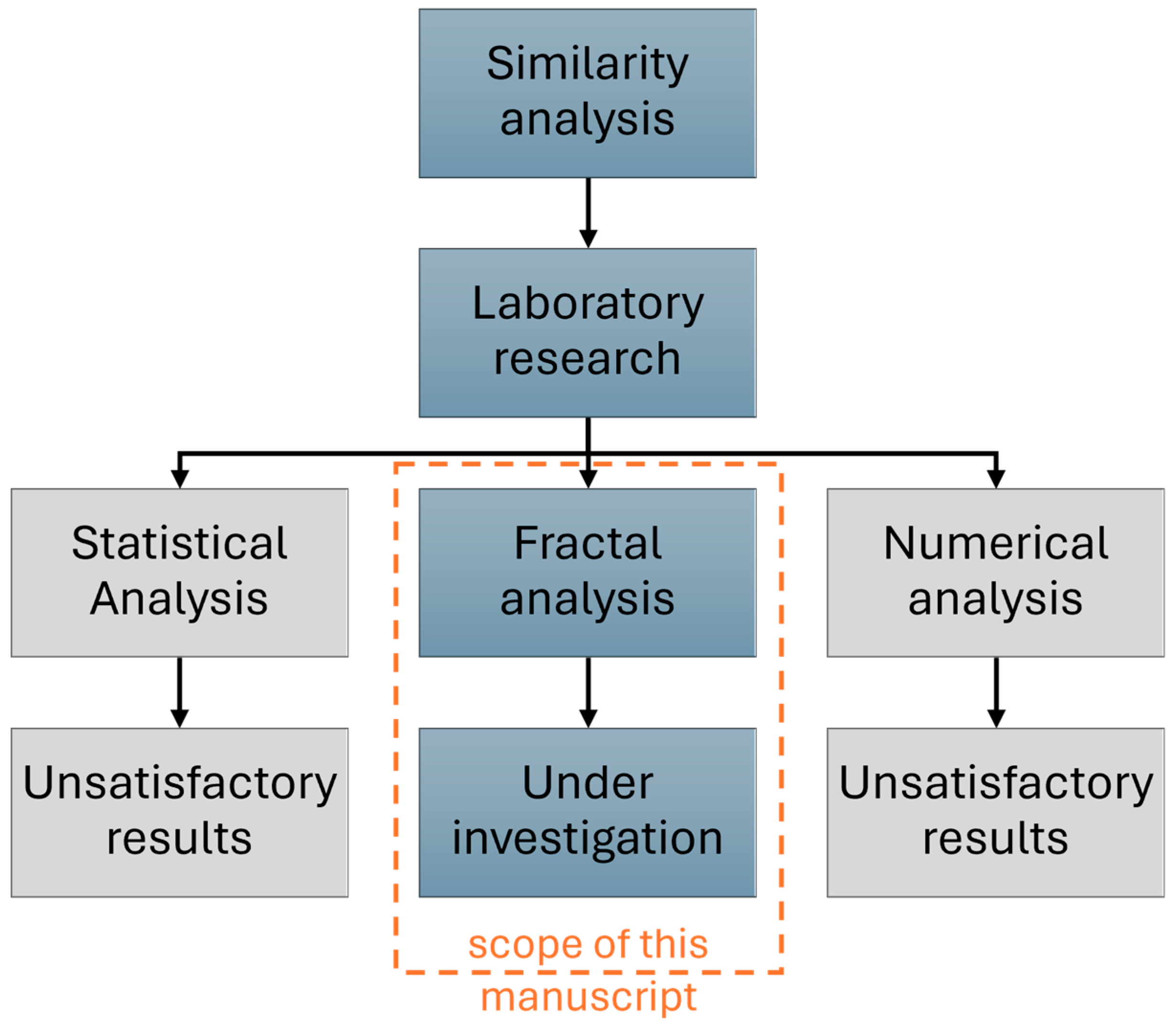
Among the proposals to limit the dangerous and costly effects of the suffosion phenomenon after a possible water pipe failure is the determination of the so-called outflow zones, within which water can flow to the soil surface after a leak occurs in a pipe. An attempt to limit the effects of a possible failure related to soil suffosion by determining an outflow zone is an alternative method to the methods aimed at preventing failures, but it should be emphasized that both approaches complement each other. However, estimating the dimensions of the outflow zones is a difficult task due to the complexity of the phenomenon in question and its dependence on many factors. The analyses presented in this article are part of larger studies aimed at determining the range of the outflow zone. The full scope of research is presented in the block diagram (Figure 1). The conducted research, based on the statistical analyses and numerical simulations presented in the works [1,2,3,4,5], did not give satisfactory results in the context of determining the range of the outflow zone; therefore, an attempt was made to determine such a zone using fractal geometry elements.
One way to determine the outflow zone is through a geometrical analysis of the distribution of points corresponding to the places of water outflow onto the soil surface. As it was shown in previous research, these points create irregular sets that are difficult to describe based on the concepts of classical Euclidean geometry [6]. Simultaneously, these sets meet the conditions for random fractals [7], so it is possible to determine their fractal dimensions. The aim of the article is to check the possibility of using a fractal dimension to estimate the size of the water outflow zone on the soil surface as a result of leakage from a water pipe. The obtained research will give direction to further analyses aimed at determining the outflow zone. It is a very important issue in terms of the safe operation of water supply systems.
2. Literature Review
2.1. The Phenomenon of Suffosion as a Result of Water Leakage from Buried Pipes
The undesirable flow of water from a buried water pipe into the soil is a common example of liquid outflow from a pressure pipe into a porous medium. Leakages from water pipes may pose a threat to the safety of people and property. The danger results from the possibility of suffosion occurrence, which is caused by the flow of water in internally unstable soil. As a result of this flow, small particles can be detached from the soil matrix and moved by water in the soil pores, causing the formation of empty spaces under the soil surface and land depressions [8].
Two conditions must be met simultaneously for the suffosion process to occur. The first, called the geometric condition, concerns the physical characteristics of the soil, and the second, the hydraulic condition, concerns the water flow. The soil meets the geometric condition of suffosion if it has granulation and pore sizes large enough to create channels inside the soil along which small particles can move. Second, the hydraulic condition for suffosion is met if the velocity of water flowing through internally unstable soil is high enough to cause the detachment of particles from the soil matrix. A verification of the hydraulic condition of suffosion requires determining the critical velocity of water flow in the soil at which particles are washed out from the soil matrix [9].
The velocity of the water leaking from the pressure pipe may be sufficient to reach a critical value. If the leakage is very intense, the changes in the soil structure characteristic for suffosion become visible very quickly. An example may be the failure of a water main, resulting in a sudden outflow of water, often visible almost immediately on the soil surface. The effects of smaller leaks, e.g., from water connections, unless the failure is repaired, may become visible on the soil surface in the form of depressions after some time (in Poland, usually after over one hundred days [10]). These depressions are usually smaller than in the case of main failures. However, situations where the flow of water from the pipe is small, is difficult to detect, where no changes are visible on the soil surface, and where the water can easily flow away, e.g., through a leak in the nearby sewage pipe, are dangerous. Then, if the leakage from the water pipe does not stop, the water washes out more and more soil particles, the empty space under the surface of the soil increases, and a dangerous sinkhole may form. Such cases have occurred many times around the world and are still being reported [11,12,13], so it is an important and current problem.
The phenomenon of suffosion is particularly dangerous in urbanized areas, because these areas are characterized by a higher population density than non-urbanized areas, with more compact and often higher buildings, as well as the presence of industrial infrastructure. Sinkholes or depressions in the land surface resulting from suffosion may therefore lead to construction disasters in these areas, posing not only a threat to human life, but also causing significant economic losses.
2.2. The Problem of Water Supply Network Failures Resulting in Leakages
The risk of suffosion in urban areas is most often associated with the presence of water supply and sewage infrastructures [11,13], because the operation of these systems is accompanied by failures resulting in the outflow of water or sewage into the ground. Leakages occur even in properly managed and maintained networks throughout all periods of their operation, presenting a problem for water and wastewater utilities around the world, in both in developing and developed countries, as shown in [14,15,16,17].
The phenomenon of water leaking from a damaged pipe into the soil is known and widely presented in the literature. Especially in the last years, there has been an increased interest in the problem of failure rates of water pipes and the need to reduce leaks. Attempts are made to predict network failure rates using mathematical and numerical methods (including machine learning, artificial neural networks, fuzzy sets, and genetic algorithms, e.g., as shown in [18,19,20,21,22,23,24,25]). Increasingly better ways of detecting and locating leaks as well as methods of limiting them are being investigated, e.g., as shown in [26,27,28,29,30,31,32,33,34,35,36]. Both direct, using the latest technologies, and indirect methods, based on water loss coefficients, for assessing the technical conditions of water pipes are constantly being improved, e.g., as in [37,38,39,40]. Detecting a leak or the possibility of its occurrence early enough can prevent dangerous changes in the soil structure resulting from the suffosion. The above-mentioned activities are therefore very important in social, economic, and ecological terms. However, they are not able to fully eliminate the problem of water supply network failures. Their occurrence cannot be completely prevented, because they are caused by many factors, which are not always human dependent and not always predictable; they are often of a random nature [41,42,43,44,45]. Moreover, the limitations of the technical and financial capabilities of many water supply companies mean that the latest methods of detecting and controlling undesirable outflows are not available to every company, and the renovation or replacement of pipes in unsatisfactory technical conditions cannot be carried out immediately. It can therefore be assumed that water leaks will continue to be a problem for many years, so it is justified to take all measures to reduce their negative effects. One of the proposals is to introduce the so-called outflow zones around places on the water pipeline where a failure would pose a particular threat to the surrounding infrastructure [5]. This approach aims to reduce the effects of soil suffosion after a possible failure, so it is a different approach than failure prevention, but it should be emphasized that both approaches complement each other.
The outflow of water onto the soil surface as a result of a water pipe failure is a complex phenomenon influenced by many physical parameters, often variable in time or space, independent or interconnected. An additional factor that increases the complexity of the phenomenon is that the occurrence of suffosion is associated with simultaneous quantitative changes in the solid, liquid, and gaseous phases of the soil medium, progressing over time. Incessantly, using various scientific achievements (e.g., RNG k-ε model, Cam-clay model, and lattice Boltzmann method), attempts are made to describe special cases of water flow through a porous medium [46,47,48,49], but there is still no mathematical description of the distance between the buried water pipe and the potential place of water outflow on the soil surface after a possible pipe failure. The mathematical description would enable the determination of outflow zones, within which a water pipe failure could result in suffosion. One of the fields of knowledge in which possibilities in this area are still unexplored is fractal geometry.
2.3. Basic Information about Fractal Structures
Fractal geometry is a relatively new field, initiated as a science in the second half of the 20th century by the works of Benoit Mandelbrot [50,51]. It uses geometric objects called fractals to describe the structures too irregular to be described using traditional Euclidean geometry. The basic feature of fractals is self-similarity, which means that a fractal is an object consisting of parts similar to the whole object (after enlarging the fragment, an image similar to the whole is obtained). Almost every infinitesimal element of a fractal consists of a very large number of other elements that are separated by spaces of variable dimensions. Other features of fractals include non-trivial (intricate) structures at any scale, recursive construction procedures (repeating the same activities in subsequent iterations), difficulty of description using the concepts of classical geometry, and analytical descriptions requiring the use of recursive relationships [52].
The fractals characterized by strict self-similarity are called classical or deterministic. The process of their construction, which involves repeating the same actions based on a carefully developed algorithm, lasts infinitely long (infinite number of iterations). However, there are many fractals in nature that show self-similarity to some extent, i.e., they consist of parts that resemble the whole, but there is no strict geometric similarity. Such fractals are called random fractals [52,53,54]. The number of iterations (steps) in the process of constructing a random fractal reflecting a real object is limited, and adding subsequent elements to the set is random.
A very important parameter characterizing a fractal is its dimension. It determines the extent to which a geometric set fills the space that bounds it and can be expressed as a non-integer number [51]. When examining the flow of water in a porous medium, it is not always necessary to reflect it using theoretical fractals. It is often enough to understand that the geometric structure of the medium is a fractal set and determine its fractal dimension. The research results described in the literature show that there are relationships between the fractal dimension and the physical and hydraulic parameters of soil, e.g., grain size composition and saturated and unsaturated conductivity coefficients [55,56,57].
Fractal geometry has become a very helpful tool used both for the characterization of complex microstructures of porous media and in theoretical analyses to determine the principles of liquid flow through these media. In recent years, the scope of interest in fractal geometry has expanded to include issues related to the design and operation of water supply networks [58]. These are not the only examples of the use of fractal geometry as a research tool. It is used in almost all fields, including computer graphics and computer science, mechanics, electronics, architecture, urban planning, material science, technology, astrophysics, agrophysics, statistics, geography, biology, medicine, psychology, genetics, economics and management, film, and music, e.g., as shown in [59,60,61,62]. There are also analyses of water flow in the ground (its physical and hydraulic parameters) in the aspects of relationships between the fractal dimension and these parameters. For example, Millán et al. [55] showed that in the soil samples they studied, with an increase in the content of clay particles, the bulk fractal dimension also increased, while an increase in the sand content in the soil was associated with a lower value of the fractal dimension. Bayat et al. [56] proved that by treating the soil as a fractal structure and using the parameters characterizing it (e.g., fractal dimension) as input data for artificial neural network models, the accuracy of the estimation of water retention curves increases significantly. The fractal dimension of soil pores can be used not only to determine the porosity [63], but also the permeability in the saturated or unsaturated state [57,64,65,66,67,68,69]. The fractal dimension of the geometric structure can also be helpful in predicting easy flow paths [70,71] and determining the erodibility of soils [72] or the degree of their degradation [73]. Attempts to use fractal geometry to describe increasingly advanced and complicated phenomena resulted in the distinction, apart from basic fractals, of objects referred to as multifractals and superfractals, which were also used in aspects of water flow through porous media [74]. In recent years, we can also observe the introduction of a new type of fractal, which is better used in the case of periodic or pseudo-periodic phenomena. The so-called “blinking fractals” were originally introduced by Sergeyev [75], and their application in water-relevant topics seems to be promising [76].
The multitude of applications of fractals, on the one hand, confirms the effectiveness of fractal geometry as a research tool, but on the other hand, it may be assumed that this field has yet untapped possibilities. This justifies an attempt to use fractal geometry to determine the zone of water outflow onto the ground’s surface as a result of the leakage from a buried water pipe.
3. Materials and Methods
As it was mentioned in the Introduction, the analyses presented in this article are part of a larger scope of research aimed at determining the range of the zone of water outflow on the soil surface after the breakage of a pipe. In order to obtain data for the analysis, it was necessary to carry out a series of laboratory tests involving a physical simulation of the failure of a buried water pipe, as a result of which water flowed onto the soil surface. The construction of the laboratory setup was preceded by the selection of parameters that have the strongest relation to the distance between the place of water outflow on the soil surface and the place of leakage from the pipe, as well as the analysis of the similarity of the phenomena (dimensional analysis) [6,77].
The water outflow locations obtained as a result of laboratory tests created real geometric structures (RSs), which were analyzed in this article. Since it was previously shown that RSs have fractal features [7], the analyses focused on their fractal dimensions (Db). To simplify the research, an RS was reduced first to a plane form (Theoretical Planar Structure, TPS) and then to a linear form (Theoretical Linear Structure, TLS) using isometric transformations. The next stage of the research was the analysis of the parameters characterizing simplified TLSs, including Db. The full scope of research is presented in Figure 2.
3.1. Laboratory Tests
Laboratory investigations of water outflow on the soil surface after an induced water pipe failure were conducted on the research setup reflecting natural conditions at a scale of 1:10. The 3D scheme of the laboratory setup is presented in Figure 3 and consisted of a cuboid box (1) filled with medium sand (7), an intentionally damaged water pipe (2) supplied with water through an elastic hose (4) from a container (3) located at the assumed height. The pipe failure was presented as a bell-and-spigot joint (7) disconnection. The cuboid box was additionally equipped with a drainage installation (5), drainage ball valves (8), and supply ball valves (9).
The laboratory research was conducted in four test series (I–IV) for the variants that differed in hydraulic conditions in the water pipe (different values of hydraulic pressure). In every series, in accordance with the standard procedures of statistical calculations of the minimum number of samples [78], each experiment was repeated 7 times under the same pressure head conditions and leak area in a pipe. The width of the leak between the spigot and socket ends of the pipe diameter equaled 15 mm, while the inner pipe diameters were DN6, DN10, DN20, DN32, and DN40 mm. Due to the loosening of the pipe connection, experiments were conducted for 5 different leak areas: 2.83 cm2, 4.71 cm2, 9.42 cm2, 15.07 cm2, and 18.84 cm2. The internal water pressure head in the water pipe (2) varied in the range 3.0÷6.0 m H2O every 0.5 m, depending on the height of the container and the water level in it. The average medium sand parameters used in experiments were as follows: compaction factor, 0.85; moisture content, 7.10% vol.; saturated hydraulic conductivity, 2.16 × 10⁻⁴ m/s; and uniformity coefficient, 3.71. The mentioned soil parameters were determined in the laboratory using standard procedures [79,80,81,82].
Each repetition of the laboratory experiment followed the same procedure. At the beginning, all valves were closed, and water was poured into the container (3) above the assumed level. Next, the supply valves (9) were opened until the water in the container reached the assumed level after the deaeration process. Then, two parts of the pipe (2) were disconnected (in the bell-and-spigot joint (7)) by pulling one end of the pipe (2), which was sticking out of the cuboid box (1). After the water had appeared on the sand surface, the valve (9) was closed, and the place of water outflow on the sand surface was localized. After the deaeration process, the experiment was video recorded nonstop.
The obtained results of the physical failure simulation allowed for the creation of data sets specifying the places of water outflow onto the ground surface. The location of the so-called suffosion holes was measured in relation to the place on the ground’s surface located directly above the leak in the pipe. The outermost outline point of a suffosion hole was taken into account. The location of each point was determined using Cartesian coordinates (x, y), with the origin (0, 0) assumed to be above the leak location in the water pipe. The distances parallel (x) and perpendicular (y) to the test water pipe were measured during the investigations. The distance (Rw) between the outermost outline point and origin was calculated on the basis of x and y. The exemplary location of the suffosion hole in the laboratory setup is presented in Figure 4. The distance Rw equaled 683.33 mm, while the x distance was equal to 566.25 mm, and the y distance was equal to 382.50 mm. Additionally, Figure 4 presents 4 main types of suffosion holes observed during the laboratory tests: (a) compact hole, (b) point hole, (c) elongated hole, and (d) fissure hole.
The points representing the suffosion holes obtained from laboratory tests, described by the x and y coordinates and the distance Rw, were grouped into sets according to the leakage area and according to the hydraulic pressure in the water pipe, creating 12 geometric structures (called Real Structures, RSs). The points obtained from physical simulations of water leaking through a hole with an area of 2.83 cm2 formed the structure F1, for a leak area 4.71 cm2: F2, for 9.42 cm2: F3, for 15.07 cm2: F4, and for 15.07 cm2: F5. Similarly, structures named H1, H2, H3, H4, H5, H6, and H7 were created as sets of points obtained as a result of water leaking from a pipe with a pressure head of 3.0, 3.5, 4.0, 4.5, 5.0, 5.5, and 6.0 m H2O, respectively. Each structure was created iteratively by adding points in subsequent repetitions of the experiment.
3.2. Simplifying the Real Structure
The simplification of the RS consisted in transforming a structure embedded in a 2D space into a structure embedded in a 1D space using isometric transformations. The process included 2 stages: creating a Theoretical Plane Structure (TPS), located in the first quadrant of the coordinate system, and transforming the TPS into a Theoretical Linear Structure (TLS), located on the positive part of the x-axis. To create a TPS based on the RS, the RS points located in the third quadrant of the system coordinates were subjected to point inversion with respect to the origin, and the RS points from the fourth and second quadrants were subjected to axial symmetry around the axes x and y, respectively. The formation of the TPS corresponding to the RS is shown in Figure 5. All points forming the TPS are described with the non-negative coordinates.
For the purposes of this work, it was assumed that the outflow zone had the shape of a circle as one of the basic centrally symmetric figures. This assumption made it possible to consider only one distance Rw for the location of each point corresponding to the suffosion holes—from the origin of the coordinate system, instead of two distances—from the x and y axes. Moreover, the number of points within a certain arbitrary range of distances from the origin was important in the research, whereas the position of the points relative to each other was not important. Thus, the second stage of simplifying the SR was to transform the TPS so that the points corresponding to the suffosion holes were located on the positive half of the x-axis, including the origin, at an unchanged (the same as for the SR) distance from the origin. For this purpose, each point was rotated by an appropriate angle around the origin, as shown in Figure 6.
The resulting structure, called a Theoretical Linear Structure (TLS), is a less complicated geometric figure than the RS or TPS, and retains all the features of the RS that are important in the study of the circular water outflow zone. All RSs obtained as a result of the laboratory tests (F1, …, F5 and H1, …, H7) were transformed into TLSs. On the basis of F1, an TLSs called F1″ was created, and similarly, on the basis of the remaining 11 RSs, linear structures F2″, …, F5″ and H1″, …, H7″ were created, respectively.
3.3. Specifying the Parameters Characterizing TSLs in Terms of the Zone Range Determination
An analysis of the nature of the distribution of suffosion holes on a plane was presented in the work [6]. The analysis consisted of checking whether a given distribution of points (suffosion holes) in a specific research area is an implementation of a uniform Poisson process, meaning complete spatial randomness. Ripley’s K function was used as a tool for analyzing the object location data. Comparing the estimator of the Ripley K function determined on the basis of laboratory tests to the theoretical value of the Ripley K function for a homogeneous Poisson point process allowed for the conclusion that the suffosion holes were randomly distributed. Therefore, it was possible to assume that TLSs, like RSs, are fractal structures, and the analysis of TLSs focused on the dimensionality of these structures. In fractal geometry, there are variously defined dimensions, but the concept of fractal dimension is often referred to the so-called box-counting dimension, the definition of which can be presented in the form [52]:
where is a non-empty, bounded subset of a finite-dimensional Euclidean space (in our investigations: = F2″, …, F5″, H1″, …, H6″ or H7″), is the box-counting dimension of the set , and is the smallest number of sets of diameter δ (in our investigations: square of side δ) which can cover .
The box dimension of the Theoretical Linear Structure was determined using a graphical method. It consists in approximating, using a straight line, the graph of the function depending on . The slope of the obtained straight line corresponds to the box-counting dimension [83]. In the analysis, it was assumed that the expression in the definition of the box-counting dimension (Equation (1)) means the number of meshes of side δ (“boxes”) intersecting or covering points of the TLS (set ). It was also assumed that the unit mesh (δ = 1) is a square with a side length of 10 cm. To create a graph of the function depending on , which is the essence of the method used to determine Db, meshes with side δ were counted in the range from 0.1 to 0.9 every 0.1. Figure 7 shows how to determine the number of meshes depending on the value of δ for an example TLS. The determined values of constituted data for the graph of the relationship between and , and thus, the basis for estimating the box-counting dimension of TLS.
The fractal dimension determines the extent to which a geometric structure fills the area limiting it [51]. This feature allows for the assumption that the fractal dimension can be used to determine the zone of water outflow onto the soil surface after a water pipe failure. In the case of the TLS, the area bounding it is a segment, one end of which coincides with the origin (the point on the soil surface located exactly above the place of water outflow from the water pipe), and the other is the point corresponding to the point of water outflow onto the soil surface, furthest from the leak in the pipe; in other words, it is a segment , the length of which equals:
where Rw is the distance of the point creating the TLS from the origin, nw and the number of points creating the TLS, and is the set of natural numbers.
For a linear structure as an object embedded in a 1D space, using the fractal dimension, it is relatively easy to determine the length of the “filled” part (marked with the symbol ) in the segment as:
In the graphical interpretation, is the length of the segment , which can be the basis for determining the radius of the water outflow zone on the ground surface after a water supply failure. The methodology for determining Db shows that the value of Db of the TLS is influenced by the distance of the points creating the TLS from the origin (the distribution of points within the segment ), as well as the number of nw points forming the TLS. If the distribution of points within the segment was uniform, the number of nw would certainly be important. However, since the distribution of points is random, the influence of nw on Db is ambiguous and requires analysis. The box-counting dimension Db, length , Rfr parameter, and the number of nw were therefore determined for each of the linear structures F1″, …, F5″, H1″, …, H6″ and H7″ as parameters important in the aspect of testing the possibility of estimating the range of water outflow zone.
4. Results and Discussion
4.1. Results of the Laboratory Tests
In 532 physical simulations of water supply failures carried out in the laboratory, a total of 662 suffosion holes were obtained, which created 12 RSs. During a single experiment, 1–5 holes occurred. Of all the holes, 10 appeared on the x-axis (i.e., directly above the test pipe) and 11 on the y-axis (on a straight line perpendicular to the pipe, passing through the leak). Taking into account the remaining 641 holes, 153 were in the first quadrant of the coordinate system, 167 in the second, 172 in the third, and 149 in the fourth. An example of the distribution of points corresponding to the suffosion holes obtained as a result of laboratory tests is shown in Figure 8. The results reflect the distribution of the suffosion holes forming the F1 structure.
On the basis of the location of the points corresponding to the suffosion holes obtained during laboratory tests, it could be concluded that the probability of water outflow is almost the same in each of the quadrants of the coordinate system: 23.1%, 25.2%, 26.0%, and 22.5% in the subsequent quadrants, respectively. The similarity of probability values is related to maintaining the repeatability of soil conditions in each quadrant at the laboratory site. This meant that the origin of the coordinate system located directly above the leak in the pipe could be treated as the center of the area, limiting the location of the suffosion holes as well as the outflow zone, which was the subject of the research, which would be a centrally symmetric figure with the point of inversion at the origin. Due to the random distribution of points, as presented in the article [6], it was difficult to characterize RSs using classical concepts of Euclidean geometry. However, the analyses performed showed that RSs have the features of random fractals [7].
4.2. Results of Simplifying the Real Structure
In the aspect of the conducted research aimed at determining the range of the zone of water outflow on the soil surface after a water pipe failure, the distance of the points from the origin was important, whereas the distances between individual points and their belonging to the quadrants of the coordinate system were irrelevant. Due to the proven randomness of the location of the points [6] and the comparability of the water outflow probabilities in individual quadrants of the system (Section 4.1), it was possible to simplify the analyzed geometric structure of an RS from the form embedded in the 2D space to the TLS form embedded in the 1D space. TLSs corresponding to all real structures F1, …, F5 and H1, …, H7 are shown in Figure 9.
Only isometric transformations of points were used to build the TLSs, which means that the distance of each point of the structure from the origin of the coordinate system remained unchanged in relation to the corresponding distance for the real structure, created based on the results of laboratory tests. A TLS as a structure created on the basis of a fractal RS retained all the features characteristic of random fractals, such as the following:
- Approximate self-similarity: This feature has been improved for RSs by enlarging individual frames of the recordings of water outflow and the formation of a suffosion hole [7]. The stages of formation of the suffosion hole were the same regardless of the location of the hole, so it can be concluded that the self-similarity condition is also met by the TLS structure.
- Non-trivial structure: It is obvious that all TLS points lie on the x-axis, but the distances of these points from the place of water leakage from the pipe (the origin) are different and non-obvious (Figure 9). The number of points creating the TLS is also non-obvious; Therefore, each TLS has a non-trivial structure.
- Recursive construction procedure: Each RS was created in consecutive steps corresponding to successive repetitions of the experiment; The TLS can also be gradually constructed based on subsequent steps of the RS creation.
- Recursive dependencies in the analytical description: The process of creating TLSs can be described by the same recursive dependency as for an RS [7]:
- Difficulty of description using Euclidean geometry concepts: Geometric figures that constitute a subset of Euclidean space, after adopting a coordinate system, can be described using a set of classical equations or inequalities that relate the coordinates of points [84]; TLS cannot be described in this way due to the randomness of points corresponding to its RL and the non-obvious number of points, creating TLSs.
- Randomness occurring in successive iterations: This feature results from the improved randomness of RSs [6], which is the basis for the creation of TLSs.
- Limited number of iterations: The number of iterations is equal to the number of repetitions of the experiment; Thus, it is limited.
4.3. Analysis of Parameters Characterizing TLS with Regard to Determining the Water Outflow Zone
Since the TLS turned out to be a fractal set, it was possible to determine its dimension Db (Figure 10) and then the distance Rfr. The values of all parameters selected for characterizing TLSs (Db, , Rfr, and nw) are summarized in Table 1 and Table 2.
When analyzing the TLSs created based on the size of the leaks in the water pipe (Table 1), the structure F3″ corresponding to leaks with an area of 9.42 cm2 showed the highest Db value. The structure with the smallest dimension was F1″, corresponding to leaks with the smallest area: 2.83 cm2. The structure F5″ corresponding to the largest leak (18.84 cm2) had a Db dimension of 0.8307, which was a relatively large value but not the highest. Therefore, no correlation was observed between the leak area in the water pipe and Db. The average dimension value for all TLSs divided according to the leak area was 0.8232. The largest value differed from it by 8.1%, while the smallest, by 6.0%. The structure F4″ had the dimension closest to the average value. In Table 1, a high coefficient of determination R2, close to 1, is notable, indicating a very good fit of the trend line (straight line), with which the box dimension is determined, to the data obtained from the experiment, simultaneously confirming the correctness of the graphical method for determining this dimension.
Analyzing the length of the segment bounding the linear structure (Table 1), as in the case of Db, there seems to be no correlation between this parameter and the leak area in the water pipe. The structure F2″ is characterized by the largest value of , while the smallest value belongs to the structure F1″, with a relatively large difference between them: 12.55 cm, which is 23.78% of the mean value of for structures F1″ to F5″, which equals 52.78 cm. Regarding Rfr, the structure F1 has the smallest value (34.74 cm). The values of Rfr for the other structures in Table 1 are approximately 10 cm larger and comparable to each other. The average value of Rfr for all structures F1″ to F5″ equals 43.46 cm, with a range of 12.04 cm (27.70% of the mean).
Similarly, when analyzing the parameters characterizing the structures corresponding to hydraulic pressure heights in the water pipe (Table 2), no dependencies were found between the analyzed parameters (Db, , and Rfr) and the pressure in the water pipe. A coefficient of determination R2 close to 1 also was observed for Db. However, the mean values of the individual parameters for all structures H1″ to H7″ are smaller than those for the parameters in Table 1, with a greater range. The mean value of Db is 0.7768. The largest value (for the set H3″) differs from the mean by 18.3%, and the smallest (for the set H7″), by 13.2%. The average value of equals 50.25 cm, with a range of 14.22 cm (28.30% of the average). For Rfr, these statistics equal 39.08 cm and 18.69 cm (47.82%), respectively.
The number of points nw creating individual TLSs varied, both for the structures presented in Table 1 and Table 2. The next step of the research was to examine whether this number affects the values of Db, and Rfr, considering all structures from Table 1 and Table 2 (Figure 11). While analyzing the scatter plot presented in Figure 11a, a slight upward trend in the relationship Db–nw can be noticed, but it is not confirmed using regression analysis. None of the analyzed trend lines (exponential, linear, logarithmic, or power) showed a satisfactory fit to the empirical points (R2 < 0.5; the best fit for the logarithmic line, R2 = 0.44, is presented in Figure 11a). Very similar results were obtained when examining the relationship as a function of nw (Figure 11b). Among the analyzed lines, the logarithmic trend line also showed the best fit, and the coefficient of determination for this line also did not exceed 0.5 (R2 = 0.42). The low value of R2 results from the number of points forming TLSs. Based on laboratory tests, the obtained structures mainly consisted of several dozen points; only two structures consisted of over 150 points. As a result, there was an accumulation of points in the left part of the trend line, hence the low R2 value, even though visually, the fit seems to be good. The detailed R2 values for Db were as follows in descending order: logarithmic, 0.4443 (best fit); power, 0.4326; polynomial, 0.4194; linear, 0.4053; and exponential, 0.3854. Analogically, the detailed R2 values for were as follows: logarithmic, 0.4234 (best fit); linear, 0.4225; exponential, 0.4216; polynomial, 0.4060; and power, 0.4052.
A significantly better fit of the trend line to the empirical data was achieved for the relationship Rfr–nw, i.e., analyzing the influence of the number of holes nw on the product of previously considered values (Figure 11c). A clear upward trend was observed. The highest coefficient of determination was obtained for the logarithmic trend line (as expected), and since this value clearly exceeded 0.6 (R2 = 0.78), the fit of this line to the empirical data can be considered satisfactory. On the basis of the considerations above, it can be concluded that the number of points forming the linear structure can have a significant impact on the analyzed parameters, especially on the value of Rfr. To assess the magnitude of this impact, it would be necessary to repeat the analysis for a larger number of different linear structures, especially those constructed from a large number of points.
5. Summary and Conclusions
To sum up, the points obtained from laboratory research corresponding to the suffosion holes were used to construct 12 Theoretical Linear Structures. Five of them were created from points divided into five groups according to the leak area in the test pipe (points belonging to one group resulted from water leakage from the pipe through a leak of the same area; all points within one group formed a single structure). Similarly, the remaining seven structures were created from points divided into seven groups according to the hydraulic pressure height in the test pipe. All constructed linear structures constituted fractal sets, so the fractal dimension (box-counting dimension) Db of each of them was determined. Additionally, the structures were characterized by three additional parameters:
- —the length of the shortest segment along the x-axis completely covering a given structure, with one end being the origin of the coordinate system;
- —the product of the fractal dimension and , which, for a structure embedded in one-dimensional space, can be interpreted as the length of the segment , completely filled by the linear structure;
- nw—the number of points creating the structure.
The values of the determined dimensions Db for individual structures ranged from 0.67 to 0.92; for , from 43.23 cm to 57.45 cm; and for , from 34.12 cm to 52.81 cm. None of the parameters showed a dependence on the area of the leak in the test pipe or on the hydraulic pressure height in this pipe. However, the influence of the number of points forming each of the linear structures on the analyzed parameters, especially on the value of , was observed. To assess the significance of this influence, it would be necessary to repeat the analysis for a larger number of different linear structures, especially those built from a large number of points. Conducting empirical research under laboratory conditions is not only time consuming but also labor intensive and costly, for example, due to the necessity of multiple replacements of compacted soil around the damaged pipe as a result of repeated experimentation. Model studies also contain certain simplifications that require special attention when generalizing the obtained research results to real conditions. In the case of the proposed physical model of water pipe failure, the limitation is the assumption of homogeneous and isotropic soil, as well as the constant leakage surface area in the pipe: in real conditions, the leakage may have a various shape and may increase during the failure. An alternative to empirical research is numerical simulations. Both the heterogeneity of the soil medium and the instability of the leak surface were taken into account in simulation studies [2,3]. In the case of points corresponding to water outflow locations on the soil surface after a water pipe failure, the distribution of which is characterized by randomness, the simulations utilizing statistical such methods as the Monte Carlo method seem most appropriate. This is the direction of the further research aimed at estimating the range of the water outflow zone after the leakage of a buried water pipe.
Author Contributions
Conceptualization, M.I.; methodology, M.I.; validation, M.I.; formal analysis, M.I.; investigation, M.I. and P.S.; data curation, M.I.; writing—original draft preparation, M.I. and P.S.; writing—review and editing, M.I. and P.S.; visualization, P.S. All authors have read and agreed to the published version of the manuscript.
Funding
This research was funded by internal projects of Lublin University of Technology, Poland, numbers FD-20/IS-6/015 and FD-20/IS-6/034.
Data Availability Statement
The data that support the findings of this study are available from the corresponding author upon reasonable request.
Conflicts of Interest
The authors declare no conflicts of interest.
References
- Iwanek, M.; Kowalski, D.; Kowalska, B.; Hawryluk, E.; Kondraciuk, K. Experimental investigations of zones of leakage from damaged water network pipes. In Urban Water II. WIT Transactions on the Built Environment; Brebbia, C.A., Mambretti, S., Eds.; WIT Press: Southampton, UK, 2014; Volume 139, pp. 257–268. [Google Scholar] [CrossRef]
- Iwanek, M.; Kowalski, D.; Kwietniewski, M. Badania modelowe wypływu wody z podziemnego rurociągu podczas awarii. (Model studies of a water outflow from an underground pipeline upon its failure). Ochr. Sr. 2015, 37, 13–17. (In Polish) [Google Scholar]
- Suchorab, P.; Kowalska, B.; Kowalski, D. Numerical Investigations of Water Outflow After the Water Pipe Breakage. Annu. Set Environ. Prot.-Rocz. Ochr. Sr. 2016, 18, 416–427. [Google Scholar]
- Iwanek, M.; Kowalska, B.; Hawryluk, E.; Kondraciuk, K. Distance and time of water effluence on soil surface after failure of buried water pipe. Laboratory investigations and statistical analysis. Eksploat. i Niezawodn.-Maint. Reliab. 2016, 18, 278–284. [Google Scholar] [CrossRef]
- Iwanek, M.; Suchorab, P.; Sidorowicz, Ł. Analysis of the width of protection zone near a water supply network. Archit. Civ. Eng. Environ. 2019, 12, 123–128. [Google Scholar] [CrossRef]
- Iwanek, M. Application of Ripley’s K-function in research on protection of underground infrastructure against selected effects of suffosion. Int. J. Conserv. Sci. 2021, 12, 827–834. Available online: https://ijcs.ro/public/IJCS-21-62_Iwanek.pdf (accessed on 15 March 2024).
- Iwanek, M. Set of Suffosion Holes Occurring After a Water Supply Failure as a Structure with Fractal Features. J. Ecol. Eng. 2022, 23, 164–171. [Google Scholar] [CrossRef]
- Wang, X.; Tang, Y.; Huang, B.; Hu, T.; Ling, D. Review on Numerical Simulation of the Internal Soil Erosion Mechanisms Using the Discrete Element Method. Water 2021, 13, 169. [Google Scholar] [CrossRef]
- Kovács, G.; Ujfaludi, L. Movement of fine grains in the vicinity of well screens. Hydrol. Sci. J. 1983, 28, 247–260. [Google Scholar] [CrossRef]
- Piechurski, F. Wykorzystanie monitoringu sieci wodociągowej do obniżenia poziomu strat wody (Using monitoring of the water supply network to reduce the level of water losses). Napędy i Sterow. 2013, 2, 66–71. (In Polish) [Google Scholar]
- Ali, H.; Choi, J.-h. Risk Prediction of Sinkhole Occurrence for Different Subsurface Soil Profiles due to Leakage from Underground Sewer and Water Pipelines. Sustainability 2020, 12, 310. [Google Scholar] [CrossRef]
- Tufano, R.; Guerriero, L.; Annibali Corona, M.; Bausilio, G.; Di Martire, D.; Nisio, S.; Calcaterra, D. Anthropogenic sinkholes of the city of Naples, Italy: An update. Nat. Hazards 2022, 112, 2577–2608. [Google Scholar] [CrossRef]
- Dastpak, P.; Sousa, R.L.; Dias, D. Soil Erosion Due to Defective Pipes: A Hidden Hazard Beneath Our Feet. Sustainability 2023, 15, 8931. [Google Scholar] [CrossRef]
- Sala, D.; Kołakowski, P. Detection of leaks in a small-scale water distribution network based on pressure data—Experimental verification. Procedia Eng. 2014, 70, 1460–1469. [Google Scholar] [CrossRef]
- Liemberger, R.; Wyatt, A. Quantifying the global non-revenue water problem. Water Supply 2019, 19, 831–837. [Google Scholar] [CrossRef]
- Taha, A.W.; Sharma, S.; Lupoja, R.; Fadhl, A.N.; Haidera, M.; Kennedy, M. Assessment of water losses in distribution networks: Methods, applications, uncertainties, and implications in intermittent supply. Resour. Conserv. Recycl. 2020, 152, 104515. [Google Scholar] [CrossRef]
- Taiwo, R.; Shaban, I.A.; Zayed, T. Development of sustainable water infrastructure: A proper understanding of water pipe failure. J. Clean. Prod. 2023, 398, 136653. [Google Scholar] [CrossRef]
- Birek, L.; Petrovic, D.; Boylan, J. Water leakage forecasting: The application of a modified fuzzy evolving algorithm. Appl. Soft Comput. 2014, 14, 305–315. [Google Scholar] [CrossRef]
- Harvey, R.; McBean, E.A.; Gharabaghi, B. Predicting the timing of water main failure using artificial neural networks. J. Water Resour. Plan. Manag. 2014, 140, 425–434. [Google Scholar] [CrossRef]
- Kutyłowska, M. Neural network approach for failure rate prediction. Eng. Fail. Anal. 2015, 47, 41–48. [Google Scholar] [CrossRef]
- Kutyłowska, M. Neural network approach for availability indicator prediction. Periodoca Polytech.-Civ. Eng. 2017, 61, 873–881. [Google Scholar] [CrossRef]
- Scheidegger, A.; Leitão, J.P.; Scholten, L. Statistical failure models for water distribution pipes—A review from a unified perspective. Water Res. 2015, 83, 237–247. [Google Scholar] [CrossRef] [PubMed]
- Boryczko, K.; Pasierb, A. Method for forecasting the failure rate index of water pipelines. In Environmental Engineering V; Pawłowska, M., Pawłowski, L., Eds.; Taylor & Francis Group: London, UK, 2017; pp. 15–24. [Google Scholar]
- Fan, X.; Wang, X.; Zhang, X.; Yu, X.B. Machine learning based water pipe failure prediction: The effects of engineering, geology, climate and socio-economic factors. Reliab. Eng. Syst. Saf. 2022, 219, 108185. [Google Scholar] [CrossRef]
- Taiwo, R.; Ben Seghier, M.E.A.; Zayed, T. Toward Sustainable Water Infrastructure: The State-Of-The-Art for Modeling the Failure Probability of Water Pipes. Water Resour. Res. 2023, 59, e2022WR033256. [Google Scholar] [CrossRef]
- Miszta-Kruk, K.; Kwietniewski, M.; Malesińska, A.; Chudzicki, J. Modern devices for detecting leakages in water supply networks. In Underground Infrastructure in Urban Areas 3; Madras, C., Kolonko, A., Nienartowicz, B., Szot, A., Eds.; CRC Press/Balkema Taylor&Francis Group: London, UK, 2015; pp. 149–161. [Google Scholar] [CrossRef]
- Okeya, I.; Hutton, C.; Kapelan, Z. Locating pipe bursts in a district metered area via online hydraulic modelling. Procedia Eng. 2015, 119, 101–110. [Google Scholar] [CrossRef]
- Karadirek, I.E. Urban water losses management in Turkey: The legislation and challenges. Anadolu Univ. J. Sci. Technol. A-Appl. Sci. Eng. 2016, 17, 572–584. Available online: https://dergipark.org.tr/tr/download/article-file/229193 (accessed on 15 March 2024). [CrossRef]
- Karathanasi, I.; Papageorgakopoulos, C. Development of a leakage control system at the water supply network of the city of Patras. Procedia Eng. 2016, 162, 553–558. [Google Scholar] [CrossRef]
- Chan, T.K.; Chin, C.S.; Zhong, X. Review of current technologies and proposed intelligent methodologies for water distributed network leakage detection. IEEE Access 2018, 6, 78846–78867. [Google Scholar] [CrossRef]
- Mohammed, E.G.; Zeleke, E.B.; Abebe, S.L. Water leakage detection and localization using hydraulic modeling and classification. J. Hydroinform. 2021, 23, 782–794. [Google Scholar] [CrossRef]
- Tariq, S.; Hu, Z.; Zayed, T. Micro-electromechanical systems-based technologies for leak detection and localization in water supply networks: A bibliometric and systematic review. J. Clean. Prod. 2021, 289, 125751. [Google Scholar] [CrossRef]
- Wu, Y.; Kang, C.; Nojumi, M.M.; Bayat, A.; Bontus, G. Current water main rehabilitation practice using trenchless technology. Water Pract. Technol. 2021, 16, 707–723. [Google Scholar] [CrossRef]
- Li, J.; Zheng, W.; Lu, C. An accurate leakage localization method for water supply network based on deep learning network. Water Resour. Manag. 2022, 36, 2309–2325. [Google Scholar] [CrossRef]
- Aslam, H.; Mortula, M.M.; Yehia, S.; Ali, T.; Kaur, M. Evaluation of the Factors Impacting the Water Pipe Leak Detection Ability of GPR, Infrared Cameras, and Spectrometers under Controlled Conditions. Appl. Sci. 2022, 12, 1683. [Google Scholar] [CrossRef]
- Rajasekaran, U.; Kothandaraman, M. A Survey and Study of Signal and Data-Driven Approaches for Pipeline Leak Detection and Localization. J. Pipeline Syst. Eng. Pract. 2024, 15, 03124001. [Google Scholar] [CrossRef]
- Maslak, V.; Nasonkina, N.; Sakhnovskaya, V.; Gutarova, M.; Antonenko, S.; Nemova, D. Evaluation of technical condition of water supply networks on undermined territories. Procedia Eng. 2015, 117, 980–989. [Google Scholar] [CrossRef]
- Gupta, A.; Kulat, K.D. A selective literature review on leak management techniques for water distribution system. Water Resour. Manag. 2018, 32, 3247–3269. [Google Scholar] [CrossRef]
- Serafeim, A.V.; Kokosalakis, G.; Deidda, R.; Karathanasi, I.; Langousis, A. Probabilistic Minimum Night Flow Estimation in Water Distribution Networks and Comparison with the Water Balance Approach: Large-Scale Application to the City Center of Patras in Western Greece. Water 2022, 14, 98. [Google Scholar] [CrossRef]
- Ramos, H.M.; Kuriqi, A.; Besharat, M.; Creaco, E.; Tasca, E.; Coronado-Hernández, O.E.; Pienika, R.; Iglesias-Rey, P. Smart Water Grids and Digital Twin for the Management of System Efficiency in Water Distribution Networks. Water 2023, 15, 1129. [Google Scholar] [CrossRef]
- Laucelli, D.; Rajani, B.; Kleiner, Y.; Giustolisi, O. Study on relationships between climate-related covariates and pipe bursts using evolutionary-based modeling. J. Hydroinformatics 2014, 16, 743–757. [Google Scholar] [CrossRef]
- Wols, B.A.; Van Daal, K.; Van Thienen, P. Effects of climate change on drinking water distribution network integrity: Predicting pipe failure resulting from differential soil settlement. Procedia Eng. 2014, 70, 1726–1734. [Google Scholar] [CrossRef]
- Rezaei, H.; Ryan, B.; Stoianov, I. Pipe failure analysis and impact of dynamic hydraulic conditions in water supply networks. Procedia Eng. 2015, 119, 253–262. [Google Scholar] [CrossRef]
- Barton, N.A.; Farewell, T.S.; Hallett, S.H.; Acland, T.F. Improving pipe failure predictions: Factors affecting pipe failure in drinking water networks. Water Res. 2019, 164, 114926. [Google Scholar] [CrossRef] [PubMed]
- Ahmad, T.; Shaban, I.A.; Zayed, T. A review of climatic impacts on water main deterioration. Urban Clim. 2023, 49, 101552. [Google Scholar] [CrossRef]
- Kissi, B.; Parron Vera, M.A.; Rubio Cintas, M.D.; Dubujet, P.; Khamlichi, A.; Bezzazi, M.; El Bakkali, L. Predicting initial erosion during the hole erosion test by using turbulent flow CFD simulation. Appl. Math. Model. 2012, 36, 3359–3370. [Google Scholar] [CrossRef]
- Wang, G.; Takahashi, A. A modified subloading Cam-clay model for granular soils subjected to suffusion. Geomech. Geoengin. 2022, 17, 1294–1308. [Google Scholar] [CrossRef]
- Abdelhamid, Y.; El Shamy, U. Pore-Scale Modeling of Fine-Particle Migration in Granular Filters. Int. J. Geomech. 2015, 16, 04015086. [Google Scholar] [CrossRef]
- Wang, M.; Feng, Y.T.; Pande, G.N.; Chan, A.H.C.; Zuo, W.X. Numerical modelling of fluid-induced soil erosion in granular filters using a coupled bonded particle lattice Boltzmann method. Comput. Geotech. 2017, 82, 134–143. [Google Scholar] [CrossRef]
- Mandelbrot, B.B. Fractals: Form, Chance and Dimension; W.H. Freeman and Co.: New York, NY, USA, 1977. [Google Scholar]
- Mandelbrot, B.B. The Fractal Geometry of Nature; W.H. Freeman and Co.: New York, NY, USA, 1982. [Google Scholar]
- Falconer, K. Fractal Geometry: Mathematical Foundations and Applications; John Wiley & Sons: Chichester, UK, 2004. [Google Scholar]
- Hassan, M.K.; Kurths, J. Can randomness alone tune the fractal dimension? Phys. A Stat. Mech. Its Appl. 2002, 315, 342–352. [Google Scholar]
- Barnsley, M.; Hutchinson, J.; Stenflo, Ö. A fractal valued random iteration algorithm and fractal hierarchy. Fractals 2005, 13, 111–146. [Google Scholar] [CrossRef]
- Millán, H.; González-Posada, M.; Aguilar, M.; Domínguez, J.; Céspedes, L. On the fractal scaling of soil data. Particle-size distributions. Geoderma 2003, 117, 117–128. [Google Scholar]
- Bayat, H.; Neyshaburi, M.R.; Mohammadi, K.; Nariman-Zadeh, N.; Irannejad, M.; Gregory, A.S. Combination of artificial neural networks and fractal theory to predict soil water retention curve. Comput. Electron. Agric. 2013, 92, 92–103. [Google Scholar] [CrossRef]
- Li, B.; Liu, R.; Jiang, Y. A multiple fractal model for estimating permeability of dual-porosity media. J. Hydrol. 2016, 540, 659–669. [Google Scholar] [CrossRef]
- Iwanek, M.; Kowalski, D.; Kowalska, B.; Suchorab, P. Fractal geometry in designing and operating water networks. J. Ecol. Eng. 2020, 21, 229–236. [Google Scholar] [CrossRef] [PubMed]
- Pothiyodath, N.; Murkoth, U.K. Fractals and music. Momentum Phys. Educ. J. 2022, 6, 119–128. [Google Scholar] [CrossRef]
- Bisht, N.; Malik, P.K.; Das, S.; Islam, T.; Asha, S.; Alathbah, M. Design of a Modified MIMO Antenna Based on Tweaked Spherical Fractal Geometry for 5G New Radio (NR) Band N258 (24.25–27.25 GHz) Applications. Fractal Fract. 2023, 7, 718. [Google Scholar] [CrossRef]
- El-Nabulsi, R.A.; Anukool, W. Modeling thermal diffusion flames with fractal dimensions. Therm. Sci. Eng. Prog. 2023, 45, 102145. [Google Scholar] [CrossRef]
- Jeong, D.P.; Montes, D.; Chang, H.C.; Hanjaya-Putra, D. Fractal dimension to characterize interactions between blood and lymphatic endothelial cells. Phys. Biol. 2023, 20, 045004. [Google Scholar] [CrossRef] [PubMed]
- Wu, J.; Yu, B. A fractal resistance model for flow through porous media. Int. J. Heat Mass Transf. 2007, 50, 3925–3932. [Google Scholar] [CrossRef]
- Xiao, B.; Fan, J.; Ding, F. Prediction of relative permeability of unsaturated porous media based on fractal theory and Monte Carlo simulation. Energy Fuel 2012, 26, 6971–6978. [Google Scholar] [CrossRef]
- Tan, X.H.; Li, X.P.; Liu, J.Y.; Zhang, G.D.; Zhang, L.H. Analysis of permeability for transient two-phase flow in fractal porous media. J. Appl. Phys. 2014, 115, 113502. [Google Scholar] [CrossRef]
- Tan, X.H.; Li, X.P.; Liu, J.Y.; Zhang, L.H.; Fan, Z. Study of the effects of stress sensitivity on the permeability and porosity of fractal porous media. Phys. Lett. A 2015, 379, 2458–2465. [Google Scholar] [CrossRef]
- Wang, S.; Wu, T.; Qi, H.; Zheng, Q.; Zheng, Q. A permeability model for power-law fluids in fractal porous media composed of arbitrary cross-section capillaries. Phys. A Stat. Mech. Its Appl. 2015, 437, 12–20. [Google Scholar] [CrossRef]
- Miao, T.; Yu, B.; Duan, Y.; Fang, Q. A fractal model for spherical seepage in porous media. Int. Commun. Heat Mass Transf. 2014, 58, 71–78. [Google Scholar] [CrossRef]
- Miao, T.; Yang, S.; Long, Z.; Yu, B. Fractal analysis of permeability of dual-porosity media embedded with random fractures. Int. J. Heat Mass Transf. 2015, 88, 814–821. [Google Scholar] [CrossRef]
- Hatano, R.; Booltink, H.W.G. Using fractal dimensions of stained flow patterns in a clay soil to predict bypass flow. J. Hydrol. 1992, 135, 121–131. [Google Scholar]
- Baveye, P.; Boast, C.W.; Ogawa, S.; Parlange, J.Y.; Steenhuis, T. Influence of image resolution and thresholding on the apparent mass fractal characteristics of preferential flow patterns in field soils. Water Resour. Res. 1998, 34, 2783–2796. [Google Scholar] [CrossRef]
- Ahmadi, A.; Neyshabouri, M.R.; Rouhipour, H.; Asadi, H. Fractal dimension of soil aggregates as an index of soil erodibility. J. Hydrol. 2011, 400, 305–311. [Google Scholar] [CrossRef]
- Xu, G.; Li, Z.; Li, P. Fractal features of soil particle-size distribution and total soil nitrogen distribution in a typical watershed in the source area of the middle Dan River, China. Catena 2013, 101, 17–23. [Google Scholar] [CrossRef]
- Veneziano, D.; Essiam, A.K. Flow through porous media with multifractal hydraulic conductivity. Water Resour. Res. 2003, 39, 1166. [Google Scholar] [CrossRef]
- Sergeyev, Y. Blinking fractals and their quantitative analysis using infinite and infinitesimal numbers. Chaos Solitions Fractals 2007, 33, 50–75. [Google Scholar] [CrossRef]
- Caldarola, F.; Maiolo, M. On the topological convergence of multi-rule sequences of sets and fractal patterns. Sofl. Comput. 2020, 24, 17737–17749. [Google Scholar] [CrossRef]
- Iwanek, M.; Malesińska, A. Zastosowanie teorii podobieństwa w modelowaniu awarii sieci wodociągowych (Use similitude in modeling water supply failure). Gaz Woda i Tech. Sanit. 2015, 3, 82–86. (In Polish) [Google Scholar]
- Tucker, H.G. An Introduction to Probability and Mathematical Statistics; Academic Press: Cambridge, MA, USA, 2014. [Google Scholar]
- American Society for Testing and Materials. ASTM D698 Standard Test Methods for Laboratory Compaction Characteristics of Soil Using Standard Effort (12,400 ft-lbf/ft3 (600 kN-m/m3)); American Society for Testing and Materials (ASTM International): West Conshohocken, PA, USA, 2021. [Google Scholar]
- American Society for Testing and Materials. ASTM D2216 Standard Test Methods for Laboratory Determination of Water (Moisture) Content of Soil and Rock by Mass; American Society for Testing and Materials (ASTM International): West Conshohocken, PA, USA, 2019. [Google Scholar]
- American Society for Testing and Materials. ASTM D3385 Standard Test Method for Infiltration Rate of Soils in Field Using Double-Ring Infiltrometer; American Society for Testing and Materials (ASTM International): West Conshohocken, PA, USA, 2018. [Google Scholar]
- American Society for Testing and Materials. ASTM E11 Standard Specification for Woven Wire Test Sieve Cloth and Test Sieves; American Society for Testing and Materials (ASTM International): West Conshohocken, PA, USA, 2022. [Google Scholar]
- Milošević, N.T.; Elston, G.N.; Krstonošić, B.; Rajković, N. Box-count analysis of two dimensional images: Methodology, analysis and classification. In 19th International Conference on Control Systems and Computer Science; Dumitrache, I., Florea, A.M., Pop, F., Eds.; IEEE Computer Society: Los Alamitos, CA, USA, 2013; pp. 306–312. [Google Scholar] [CrossRef]
- Empacher, A.B.; Sęp, Z.; Żakowska, A.; Żakowski, W. Short Dictionary of Mathematics; Wiedza Powszechna: Warsaw, Poland, 1975. (In Polish) [Google Scholar]
Figure 1.
The research scope of the zone range determination of water outflows after a pipe failure.
Figure 1.
The research scope of the zone range determination of water outflows after a pipe failure.

Figure 2.
Block diagram of research of determining the outflow zone.

Figure 3.
A 3D scheme of the laboratory setup (1—cuboid box, 2—water pipe, 3—water contained, 4—elastic hose, 5—drainage installation, 6—medium sand, 7—bell-and-spigot joint, 8—drainage ball valves, and 9—supply ball valves).
Figure 3.
A 3D scheme of the laboratory setup (1—cuboid box, 2—water pipe, 3—water contained, 4—elastic hose, 5—drainage installation, 6—medium sand, 7—bell-and-spigot joint, 8—drainage ball valves, and 9—supply ball valves).

Figure 4.
Exemplary location of the suffosion hole (left) and 4 main types of suffosion holes observed during the laboratory test: (a) compact hole, (b) point hole, (c) elongated hole, and (d) fissure hole.
Figure 4.
Exemplary location of the suffosion hole (left) and 4 main types of suffosion holes observed during the laboratory test: (a) compact hole, (b) point hole, (c) elongated hole, and (d) fissure hole.

Figure 5.
TPS creation. O1–O5—points of SR; O1′–O5′—points of TPS.

Figure 6.
TLS creation. O1′–O5′—points of TPS; O1″–O5″—points of TLS.

Figure 7.
Theoretical Linear Structure with boxes of side δ = 0.4, δ = 0.2 and δ = 0.1, covering TLS.
Figure 7.
Theoretical Linear Structure with boxes of side δ = 0.4, δ = 0.2 and δ = 0.1, covering TLS.

Figure 8.
Structure F1 as an example of an RS obtained during laboratory tests.

Figure 9.
TLSs corresponding to RSs obtained based on laboratory research.

Figure 10.
The H7″ structure covered with a grid of meshes with side lengths δ = 0.8, δ = 0.4, and δ = 0.2, with Db determined as the slope of the line approximating the graph –(−log δ).
Figure 10.
The H7″ structure covered with a grid of meshes with side lengths δ = 0.8, δ = 0.4, and δ = 0.2, with Db determined as the slope of the line approximating the graph –(−log δ).

Figure 11.
Relationship between the parameters characterizing TLS ((a) Db, (b) (Rw)max, and (c) Rfr) and the number of nw points forming TLS.
Figure 11.
Relationship between the parameters characterizing TLS ((a) Db, (b) (Rw)max, and (c) Rfr) and the number of nw points forming TLS.


Table 1.
Characterization of TLSs for data obtained from laboratory research, divided according to the leak area.
Table 1.
Characterization of TLSs for data obtained from laboratory research, divided according to the leak area.
| TLS | Leakage Area, cm2 | Db | R2 for Db | (Rw)max, cm | Rfr, cm | nw |
|---|---|---|---|---|---|---|
| F1″ | 2.83 | 0.7737 | 0.9931 | 44.90 | 34.74 | 86 |
| F2″ | 4.71 | 0.7987 | 0.9970 | 57.45 | 45.89 | 135 |
| F3″ | 9.42 | 0.8902 | 0.9858 | 48.90 | 43.53 | 109 |
| F4″ | 15.07 | 0.8227 | 0.9944 | 56.35 | 46.36 | 91 |
| F5″ | 18.84 | 0.8307 | 0.9967 | 56.32 | 46.78 | 240 |
Table 2.
Characterization of TLSs for data obtained in laboratory research, divided according to hydraulic pressure height.
Table 2.
Characterization of TLSs for data obtained in laboratory research, divided according to hydraulic pressure height.
| Data Set | Leakage Area, cm2 | Db | R2 for Db | (Rw)max, cm | Rfr, cm | nw |
|---|---|---|---|---|---|---|
| H1″ | 3.0 | 0.7524 | 0.9856 | 48.90 | 36.79 | 56 |
| H2″ | 3.5 | 0.6911 | 0.9858 | 49.38 | 34.12 | 57 |
| H3″ | 4.0 | 0.9193 | 0.9990 | 57.45 | 52.81 | 333 |
| H4″ | 4.5 | 0.7333 | 0.9877 | 47.64 | 34.94 | 62 |
| H5″ | 5.0 | 0.8423 | 0.9858 | 43.23 | 36.41 | 50 |
| H6″ | 5.5 | 0.8246 | 0.9927 | 50.35 | 41.52 | 57 |
| H7″ | 6.0 | 0.6746 | 0.9793 | 54.80 | 36.97 | 47 |
Disclaimer/Publisher’s Note: The statements, opinions and data contained in all publications are solely those of the individual author(s) and contributor(s) and not of MDPI and/or the editor(s). MDPI and/or the editor(s) disclaim responsibility for any injury to people or property resulting from any ideas, methods, instructions or products referred to in the content. |
© 2024 by the authors. Licensee MDPI, Basel, Switzerland. This article is an open access article distributed under the terms and conditions of the Creative Commons Attribution (CC BY) license (https://creativecommons.org/licenses/by/4.0/).
Share and Cite
MDPI and ACS Style
Iwanek, M.; Suchorab, P. Fractal Characteristics of Water Outflows on the Soil Surface after a Pipe Failure. Water 2024, 16, 1222. https://0-doi-org.brum.beds.ac.uk/10.3390/w16091222
AMA Style
Iwanek M, Suchorab P. Fractal Characteristics of Water Outflows on the Soil Surface after a Pipe Failure. Water. 2024; 16(9):1222. https://0-doi-org.brum.beds.ac.uk/10.3390/w16091222
Chicago/Turabian StyleIwanek, Małgorzata, and Paweł Suchorab. 2024. "Fractal Characteristics of Water Outflows on the Soil Surface after a Pipe Failure" Water 16, no. 9: 1222. https://0-doi-org.brum.beds.ac.uk/10.3390/w16091222
Note that from the first issue of 2016, this journal uses article numbers instead of page numbers. See further details here.