Assessment of Nitrogen Inputs into Hunt River by Onsite Wastewater Treatment Systems via SWAT Simulation


1
Department of Geosciences, University of Rhode Island, Kingston, RI 02881, USA
2
Department of Biological Sciences, University of Rhode Island, Kingston, RI 02881, USA
*
Author to whom correspondence should be addressed.
Water 2017, 9(8), 610; https://0-doi-org.brum.beds.ac.uk/10.3390/w9080610
Submission received: 15 June 2017
/
Revised: 20 July 2017
/
Accepted: 8 August 2017
/
Published: 16 August 2017
(This article belongs to the Special Issue Integrated Soil and Water Management: Selected Papers from 2016 International SWAT Conference)
Abstract
:Nonpoint source nitrogen pollution is difficult to effectively model in groundwater systems. This study aims to elucidate anthropogenic nonpoint source pollution discharging into Potowomut Pond and ultimately Narragansett Bay. Hydrologic modeling with Soil and Water Assessment Tool (SWAT) and SWAT Calibration and Uncertainty Program (SWAT-CUP) was used to simulate streamflow and nitrogen levels in the Hunt River with and without onsite wastewater treatment systems (OWTS). The objective of this study was to determine how input of OWTS data impacts nitrogen loading into the Hunt River Watershed in Rhode Island, USA. The model was simulated from 2006 to 2014, calibrated from 2007 to 2011 and validated from 2012 to 2014. Observed streamflow data was sourced from a US Geological Survey gauge and nitrogen loading data from University of Rhode Island Watershed Watch (URIWW). From the results, adding OWTS data to the SWAT simulation produced a better calibration and validation fit for total fit (Nash–Sutcliffe Efficiency (NSE) = 0.50 calibration, 0.78 validation) when compared with SWAT simulation without OWTS data (NSE = −1.3 calibration, −6.95) validation.
1. Introduction
Eutrophication poses a severe threat to coastal waters on local, regional, and global scales. Coastal ecosystems are naturally nitrogen limited and runoff from terrestrial systems from agriculture, wastewater, and industrial practices contributes to eutrophic areas of low dissolved oxygen, known as dead zones [1]. Dead zones have been documented as doubling in occurrence every decade since the mid 1900s and have been increasing in areal extent. Factors such as rising ocean temperatures, increasing ocean acidification, sea-level rise, and changing climate variables are acting synergistically to exacerbate the eutrophication problem [2]. Often, eutrophication, leading to conditions of hypoxia and anoxia in coastal waters, is overlooked until broad scale detrimental effects are obvious [3]. The breakdown of coastal fisheries and large fish kills garner the most attention to eutrophic conditions. Fisheries located in shallow coastal waters are the most at risk and instances of fishery and shellfish closures have increased in recent years.
Narragansett Bay, located in the state of Rhode Island (RI), USA is no exception to the problem of excess nitrogen (N) and resulting eutrophication of coastal waters. Areas of the bay have experienced N inputs for over the past 200 years and impacted areas have expanded in extent as the state’s population has grown and development has increased throughout the state. Rhode Island is the smallest state and is the second most densely populated with roughly one million residents [4]. Over the past several decades, the bay has ranked as one of the most heavily fertilized estuaries in the USA with the majority of nutrients originating from point sources [5,6]. The largest point source contributor is sewage treatment plants (STPs) [6] in the northern portion of the bay where the state capitol is located and the population density is highest. Through the years, the state has faced harmful algal blooms stemming from eutrophication, leading to fisheries and beach closures, most often during the peak summer tourism season. Both fisheries and tourism are vital to the state’s economy. In 2003, the state experienced a severe fish kill with over one million menhaden, and other finfish and shellfish, killed from anoxic conditions within Greenwich Bay, which is a smaller offshoot of Narragansett Bay [7]. This event spurred initiative for action to clean up pollution within the bay and to combat excess N from entering the state’s coastal waters in order to reduce risks to the health of the coastal ecosystems and the communities that rely upon them. Targeting the N point sources, the state set a goal of 50% reduction of N discharge into the bay from 1995 to 1996 levels, limiting the allowable discharge volumes of N from 11 wastewater treatment facilities in upper Narragansett Bay. The targeted reduction was achieved through stages by 2012 [8]. Today, as N inputs decline from point sources, nonpoint sources, such as urban runoff from septic systems, are becoming a proportionately larger contributor of N into the bay. In RI, 30% of homes are on septic systems, also known as onsite wastewater treatment systems (OWTSs) [8,9]. For coastal watersheds with households served predominantly by OWTSs, these systems can serve as significant sources of N which can contribute to detrimental eutrophication of coastal waters.
The Hunt River and two of its tributaries (Fry Brook and Scrabbletown Brook), lie within coastal watersheds served predominantly by OWTSs. These waterbodies were listed as 303 (d) Group 1, under the Clean Water Act for highest priority impacted waters in RI. The Hunt River and its tributaries have made the 1998 303 (d), under the Clean Water Act list of impaired waterbodies for several years for being impacted by fecal coliform. The majority of high bacteria counts were found to occur during wet weather conditions. The 2001 total maximum daily loads (TMDL) report determined the largest wet weather source of fecal coliform to be stormwater runoff. Fecal coliform monitoring is often used as indication of pathogen presence; however, modeling fecal coliform in freshwater systems holds a unique set of challenges. Bacteria fate and transport relies heavily on the nature of pollution events and sensitivity of fecal coliform to environmental conditions [10]. Leaking sewer and septic infrastructure greatly contributes to nonpoint nitrogen pollution to urban watersheds
In order to protect the health of any coastal community, it is important to quantify the influence of STPs and OWTSs on groundwater flow and the contributions of nutrients from these systems to coastal waters. For mitigation purposes, it is helpful to model these inputs on local watershed scales to identify potential areas of high N inputs to target for reduction through policies and infrastructure development. Few studies have been conducted modeling nutrient inputs on the watershed scale using the Soil Water Assessment Tool (SWAT) due to complexities stemming from the uncertainty of differences in subsurface hydrology, soil and water dynamics, and the often lack of detailed information about OWTS [11]. Increased densities of OWTS have been shown to increase baseflow within a watershed system [12,13,14], which can have the effect of increasing nutrient loading into ground and surface waters, eventually entering into coastal waters. OWTSs have a biozone layered designed to filter out nutrients, preventing their leaching into the groundwater. However, these biozone layers can become ineffective over time, resulting in an increased discharge of nutrients into sensitive coastal waters. Nutrient loading into a waterbody depends on local surrounding conditions, thus it is helpful to conduct modeling on smaller scales to identify areas to target for N mitigation.
In this study, we modeled the amount of N entering into Narragansett Bay on the watershed scale, with focus on the Hunt River Watershed. The Soil Water Assessment Tool (SWAT) was used to model N inputs into Potowomut Cove, which is fed by the Hunt River, and connects to Narragansett Bay. The effects on receiving waters due to nonpoint source loads, including OWTS could be effectively modeled using SWAT. The development and application of hydrologic models such as SWAT could therefore be used for the Hunt River Watershed to determine Best Management Practices (BMPs). We used a gauged watershed to calibrate the SWAT model, and estimate streamflow and nutrient loading into the bay. Recent development in the SWAT model allows the users to account for presence of septic systems or OWTSs. SWAT modeling also is unique in its ability to account for both watershed and in-stream processes.
2. Materials and Methods
2.1. Study Area and SWAT Model Description
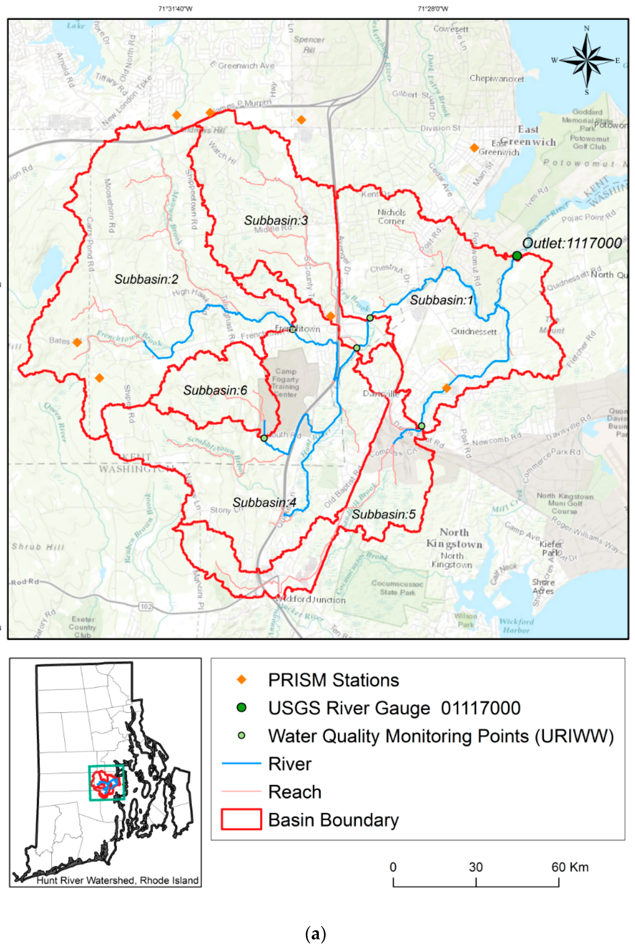
The Hunt River Watershed, as shown in Figure 1, is a small-scale (59.9 km2) watershed that cuts across central Rhode Island, USA. The 11 kilometer Hunt River winds through several towns and ultimately discharges through rural East Greenwich and into Potowomut Pond. From there, the river known as Potowomut River flows southeasterly into Potowomut Cove and then into Narragansett Bay. While the watershed is predominantly rural and undisturbed, rapid urbanization along the waterway has driven significant increases in anthropogenic pollutants. The SWAT model is hydrologic modeling software developed by the United States Department of Agriculture (USDA). The SWAT model was originally developed to predict impact of land management on water, nutrients and sediments of large ungauged basins. It was created as physically based, continuous, and computationally efficient models [15,16]. In SWAT, the catchment area is subdivided into subbasins, river reaches and hydrological response units (HRUs). Further subdivisions of HRUs are statistically performed by considering a determined percentage of subbasin area that is independent of location within the subbasin. SWAT uses a different routing scheme for runoff and chemistry through watersheds while maintaining water balance for each watershed sector. Normally, the routing for chemical transport includes sediments, erosion, plant growth, pesticides and nutrients. Modeling in-stream nutrient processes is valuable for simulating more accurate environmental conditions. A nutrient process in SWAT includes fate and transport of numerous nitrogen and phosphorus pools including organic and inorganic forms in soil and stream. The SWAT in-stream water quality algorithms incorporate nutrient interactions and relationships used in the Enhanced Stream Water Quality Model (QUAL2E) [17]. Recent advancements in SWAT modeling consider nutrient processes from OWTSs based on a biozone algorithm [18]. This algorithm is a function of the net growth of septic biomass dependent upon soil temperature and the leaching of soluble phosphorus through soil layers.
2.2. SWAT-CUP Model Description
The SWAT Calibration and Uncertainty Program (SWAT-CUP) is widely used for SWAT model calibration and uncertainty analysis. This program offers various calibration algorithms, of which, Sequential Uncertainty Fitting (SUFI2), a robust method compared to deterministic and stochastic method [19], is used for this study. The SUFI2 approach was implemented due to its comprehensive consideration of uncertainty sources in static input variables. Moreover, it gives the 95% probability distribution model output variables based on propagation of uncertainty, often referred to as 95% Prediction Uncertainty (95 PPU).
2.3. Input Data and Model Preparation
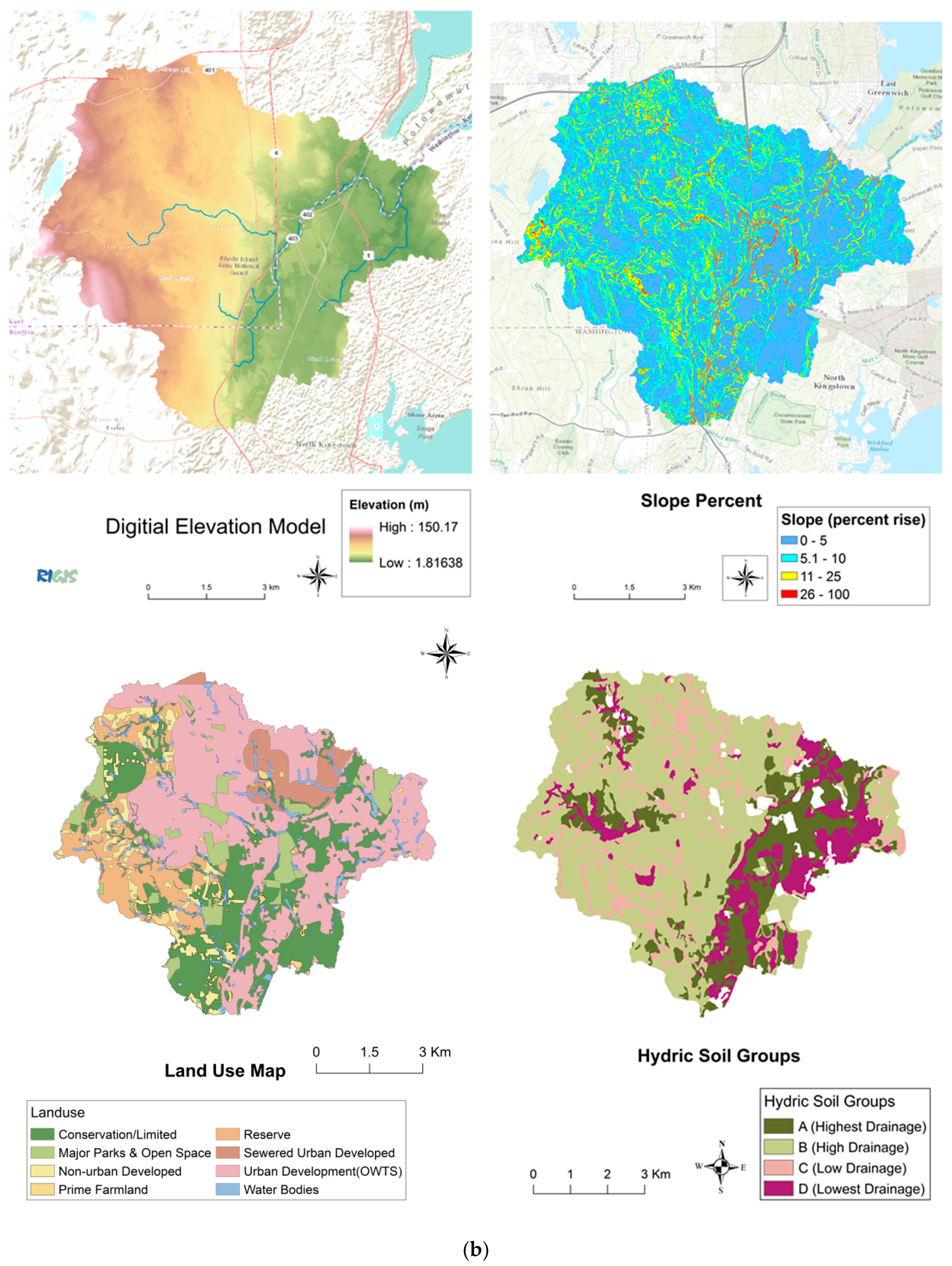
Numerous data sources were used to develop the SWAT model. Land cover data and soil data were obtained from the Rhode Island Geographic Information System (RIGIS) [20]. Precipitation data was acquired through the Parameter-elevation Regressions on Independent Slopes Model (PRISM) climate mapping system [21]. The spatial coverage representing the watershed area which included eight data stations of precipitation and temperature were downloaded from PRISM. Streamflow was calibrated using USGS Gauge 01117000 (41°38′28′′, −71°26′42′′), located in North Kingstown, Rhode Island, 4 kilometers upstream from the mouth of Narragansett Bay. The National Elevation Dataset was downloaded for the Hunt River Watershed at a 10 m resolution (U.S. Geological Survey). Official Soil Series Descriptions data was obtained from the Natural Resources Conservation Service (NRCS) Soil Survey Geographic Database (SSURGO) [22]. Land Use/Land Cover (LULC) data was obtained from the United States Geological Survey (USGS) 2006 National Land Cover Dataset (NLCD) [23] in 30 m resolution. Elevation data was obtained from Digital Elevation Model (DEM) obtained from United States Geological Survey National Elevation Data (NED) [24].
LULC data indicated that the land within the watershed delineation was dominated by forested and urban areas. The headstream of the Hunt River is predominantly urbanized (Figure 1).
According to the LULC classification system, the watershed area is dominantly classified as “Urban Development” (34%), and “Sewered Urban Area” (26%). Subbasins 1 and 5 are preeminently urbanized, whereas subbasins 2–4, and 6 are a mixture of urban development and undisturbed habitat. In respective order from highest to lowest, the remaining land use classifications identified in the Hunt River Watershed were “Major Parks and Open Space” (18%), “Conservation and Limited” (12%), “Reserve” (6%), and “Non-urban Development” (3%). Land classified as “Water Bodies” and “Prime Farmland” were both identified at less than 1%. OWTS information is not publicly available for the state of Rhode Island. In order to estimate the number of households on OWTS, sewer line data from RIGIS [25] was overlaid on the Hunt River Watershed area to determine the sewered areas of the delineated watershed using ArcGIS (ESRI—version 10.3.1). Urban areas served by sewers were subtracted from the map area to estimate land area serviced by OWTSs. Using this method, an estimated 94% of households (13.36 km2) residing on urban land within the watershed do not have access to sewer, and were therefore classified as relying on OWTS for the purpose of this study. There are no industrial waste water treatment facilities within the delineated watershed. Due to absence of agricultural land use, nitrogen inputs from fertilizers, farmland, and livestock were negligible and not included within the model.
A challenging aspect of modeling nutrients in Rhode Island is lack of continuous sampling data. This project used data from the University of Rhode Island Watershed Watch (URIWW) program, collected from five monitoring stations located along the Hunt River. The URIWW is a volunteer, citizen-science program which conducts statewide monthly water quality sampling from May–October each year, beginning in 2007 for the Hunt River [26]. Total nitrogen (TN) data collected from 2007 to 2014 was used for this study.
2.4. Model Setup and HRU Definitions
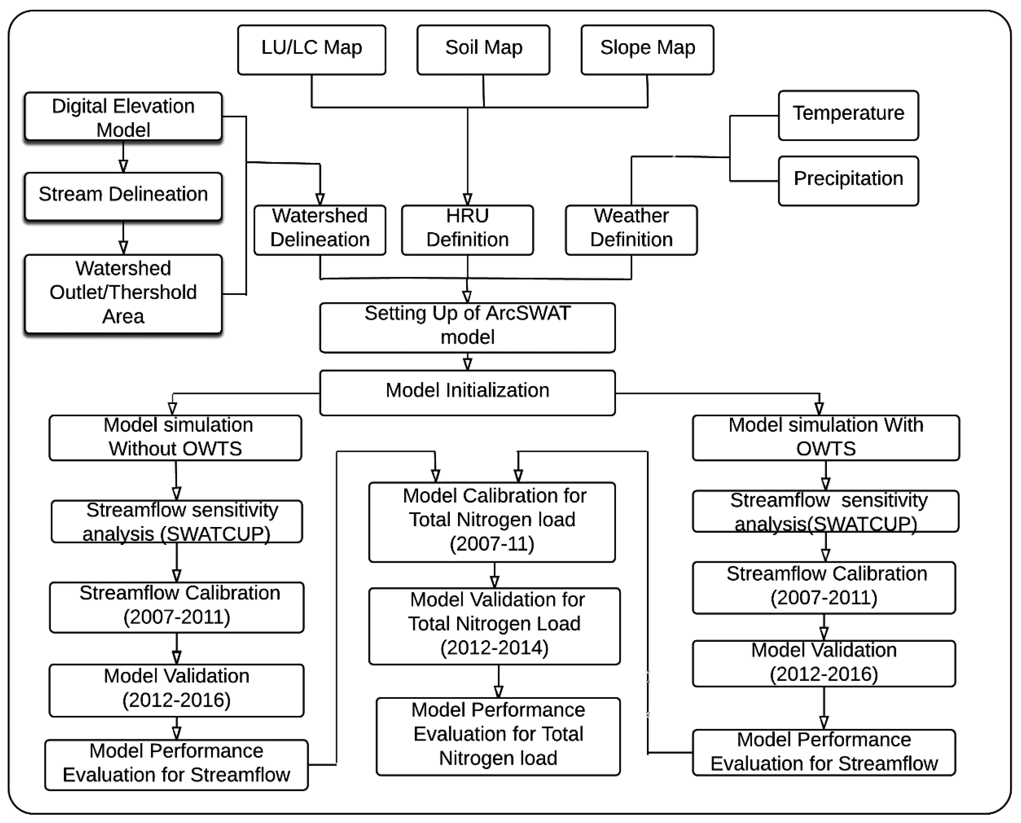
For this study, six outlet subbasins were created based on data from URIWW monitoring stations of TN (Figure 1). Subbasins were divided into HRUs by assigning threshold values of land use and land cover, soil, and slope percentage (Figure 2). Development of HRUs determines the land use/soil/slope class combinations in the delineated subbasins based on predetermined threshold values. Thresholds are typically chosen based on SWAT model objectives. Because the scope of this project focuses on OWTSs in urban areas, the thresholds needed to be small enough to recognize the fragmented urban areas within each subbasin. Therefore, HRU definitions were set at 5% land use, 5% soil, and 5% slope percentage. These small-scale thresholds yielded 320 HRUs within the six subbasins. The SWAT model was run with two distinct simulations to determine the effects of OWTS on modeling streamflow and nitrogen inputs. Changing the status of septic systems was done by changing the “isep_opt” value from 0 to 1. Other OWTS input parameters were considered as default which is as shown in the Table 1. The OWTS variable in SWAT (isep = 1) converted the urban areas within subbasin 1 to active septic system users. Both scenarios were simulated for 36 years, from 1981 to 2016, following the SWAT model setup illustrated in Figure 3. The warm up period for the model was used by one year. The observed data for Total Nitrogen data was used the years 2007 to 2016 for the simulation period. The timespan for calibration and validation was confided by the availability of streamflow and TN data. The calibration was completed with 30 TN data points, and validated with 19 TN data points.
2.5. Model Evaluation Performance
Model evaluation performance through statistical analysis is crucial. Evaluation recommendations prescribed by previous work [15,27] were used for this study. The three major categories of quantitative statistics were standard regression, Nash and Sutcliffe dimensionless, and error index [28,29]. Coefficient of determination (R2), Nash and Sutcliffe Efficiency (NSE), and percent bias (PBIAS) were used for model prediction in this study [15]. Coefficient of determination (R2) was used for standard regression analysis by describing the degree of collinearity between simulated and measured data. Values for the coefficient of determination range from −1 to 1, with 1 indicating a perfect linear relationship, and 0 indicating no linear relationship.
The NSE is a dimensionless statistical measure that indicates the magnitude of residual variance to measured variance through normalized statistics [28]. The NSE values may range between −∞ and 1, with 1 being completely inclusive. Values between 0.0 and 1.0 are generally acceptable values for SWAT models [15]. Percent bias (PBIAS) is an error index analysis that measures the average tendency of simulated data to be larger or smaller than their observed counterparts [30]. The optimal PBIAS value is 0.0, with lower values indicating accurate model simulation. Positive PBIAS values indicate model under-simulation bias, whereas negative values indicate overestimation bias [30].
3. Results
3.1. Model Sensitivity, Calibration and Validation
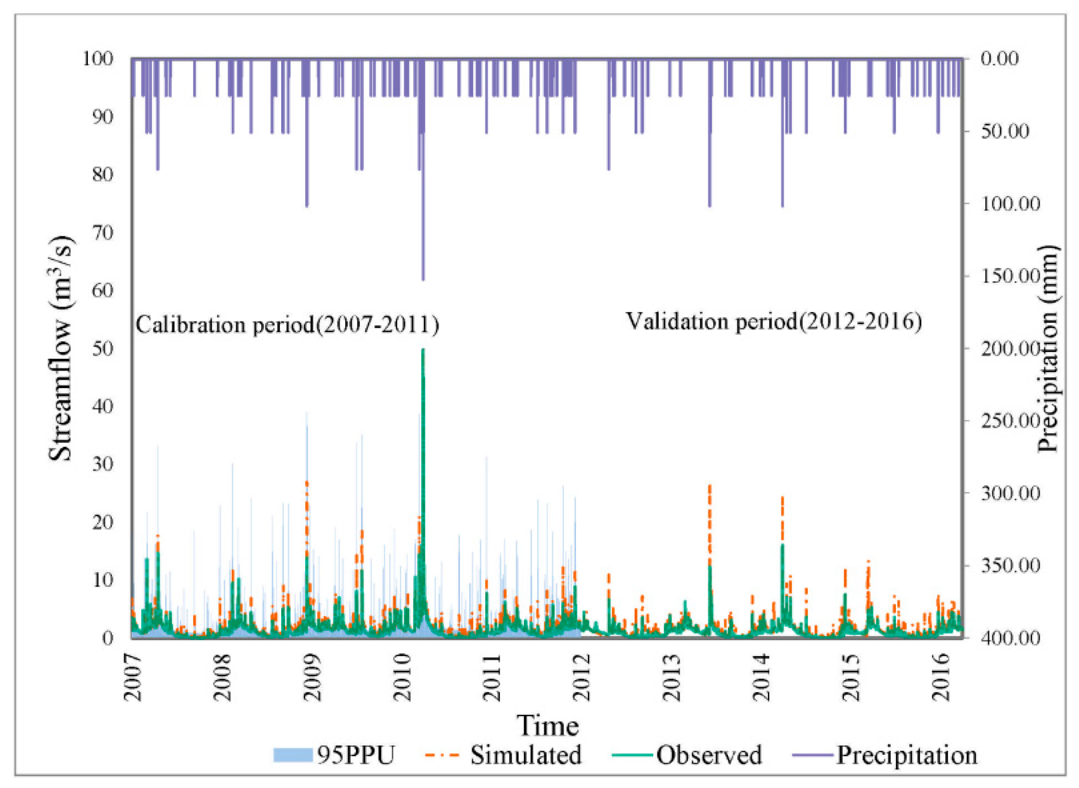
Nine hydrologic parameters were used in SWAT-CUP to calibrate streamflow. The parameters, fitted value, range of parameter and P-value are presented in Table 2 and Table 3. In the model, 1000 iterations were used for a 6-year simulation including a one-year warm-up period, with the 48th iteration yielding the best results. The two simulations analyzed in this study were streamflow and N loadings with and without OWTSs. In both simulations, the hydrologic parameters selections were identical. Sensitivity of parameters is determined by identifying the lowest values for the parameter “p-Value”. The “p-Value” serves as an indicator for sensitivity significance. By evaluating the p-Values, Table 2 and Table 3 indicate that CN2 is sensitive both with and without OWTS simulation. Other sensitive parameters include GWQMN and REVAPMN for simulation without OWTS and GW_DELAY and GW_REVAP for simulation with OWTS. In both simulations, curve Number and groundwater parameter were common sensitive parameters and influenced more surface runoff and base flow. In this study, the BFlow separation tool was used to determine the initial Alpha_BF [31]. As shown in both Table 2 and Table 3, a higher ALPHA_BF value indicates higher base flows and lower GWQMN resulted in lower base flows [11,16]. Finding optimal values for ALPHA_BF and GWQMN ensures that the streamflow is separated well to account for runoff and baseflow.
Figure 3 illustrates the observed streamflow, simulated streamflow, precipitation, and 95 PPU. Table 4 shows all nitrogen parameters that were used in the total nitrogen calibration. Statistical analysis for model calibration and validation is shown in Table 5 and Table 6. Model fit value is classified as “very good” [15] for stream calibration, with daily NSE of 0.75 and R2 of 0.78 (Table 5). For the validation period, model fit was decreased with a NSE value of 0.4 and R2 of 0.68. Overall, model performance was better for streamflow calibration in both scenarios. Meteorological forcing plays an important role in hydrologic model performance. Better spatial representation of precipitation data such as data from PRISM and temperature data ensures higher model performance compared to the NCEP dataset [32]. The average precipitation for the Hunt Watershed is 1270 mm per year. Our model’s average precipitation value was overestimated by 1367 mm per year, which could be due to Rhode Island’s 2010 flood event. With fitted parameters, the model was simulated again from January 2012 to August 2016 for validation. Validation indicated that simulated flow was overestimated by 4% which is indicated by smaller NSE values compared to the calibration period. This change in model performance could be attributed to the presence of a dry year in the validation period; however, the model captured peak flow and remained consistent with the precipitation pattern. According to the 95 PPU plot (Figure 3), the uncertainty band was narrow for stream flow’s calibration period, ranging between 34% and 50% on a daily basis.
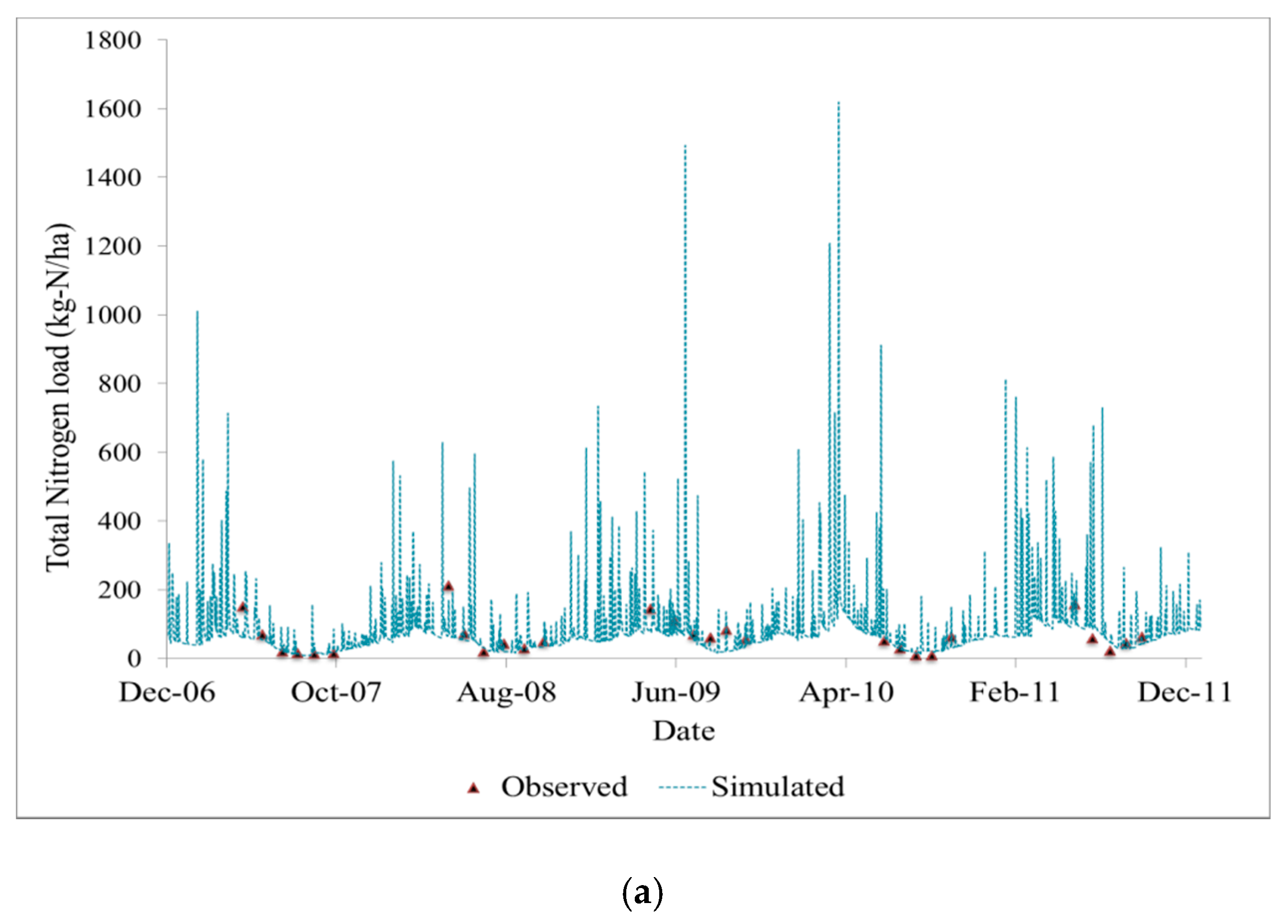
Total nitrogen was calibrated and validated after streamflow was calibrated. Nitrogen data, obtained from URIWW, was collected weekly from the months of May through October of each year. Figure 4 show the calibration and validation of total nitrogen load using SWAT model. NSE, percent bias, and coefficient of determination were calculated on a daily basis dependent on available data from URIWW. A few particular point data were overestimated; however, the overall data fit was acceptable. The model performance for total nitrogen loads for both simulations is shown in Table 5 and Table 6. For the calibration period in the presence of OWTS, the model fit was satisfactory [15] with NSE of 0.5, R2 of 0.5, and PBIAS of around 4%. For the validation period in the presence of OWTS, the model fits were very good with NSE of 0.78, R2 of 0.81 and PBIAS of around 7%. Without the presence of OWTS, model fit was poor with R2 of 0.14, negative NSE values, and high percentage bias. According to Moriasi, negative NSE, high percentage bias, and R2 < 0.5 are considered as very poor calibration [15]. The septic tank is a better reflection of nitrogen over the watershed.
3.2. Influence of OWTS on Hydrologic Cycle
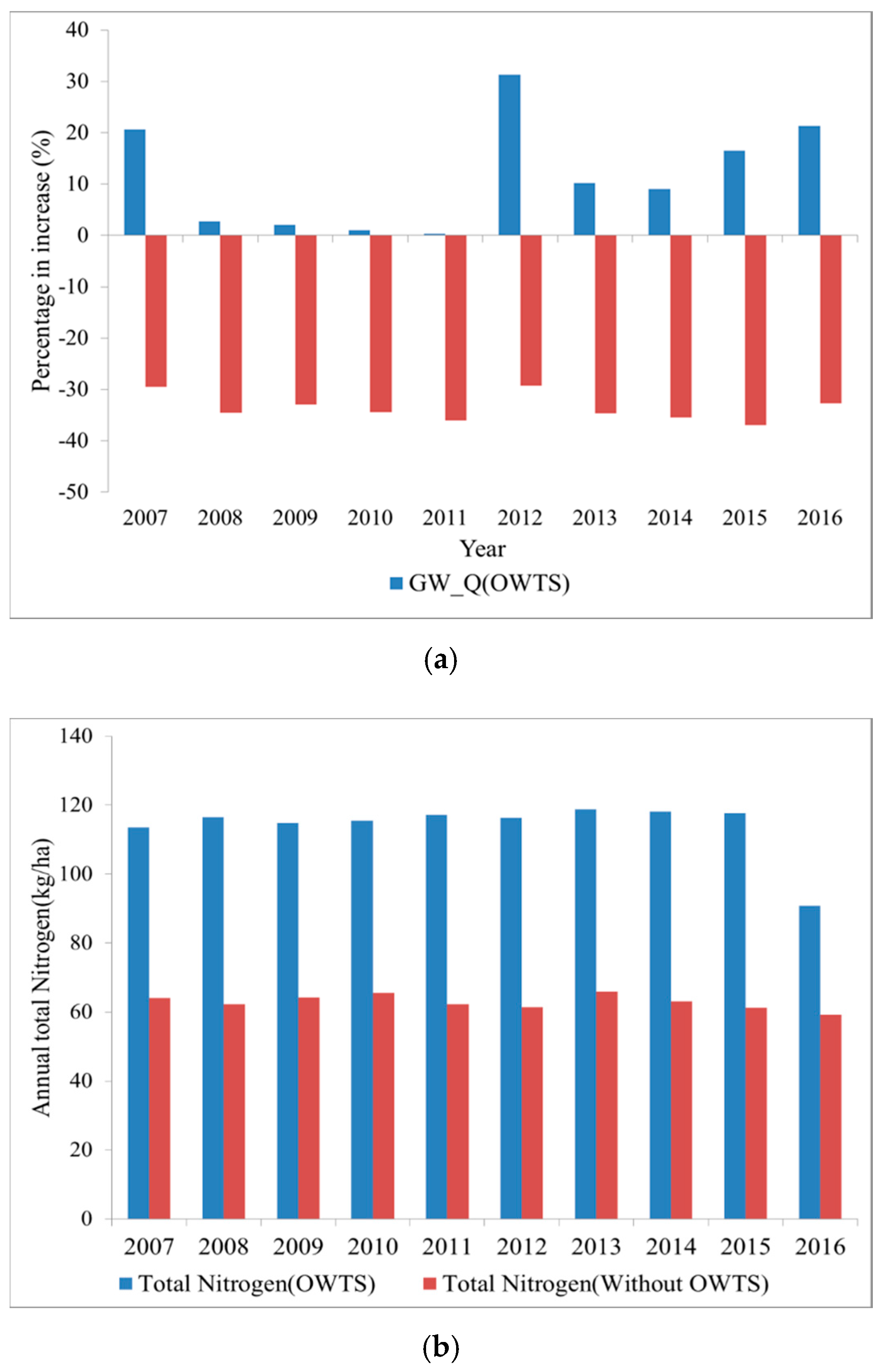
Figure 5a shows the percent increase in groundwater contributing to streamflow with and without OWTS scenarios. When OWTS data was included, groundwater contribution to streamflow at the outlet was increased for each year of simulation. The annual precipitation from 2008 to 2011 was roughly 1500 mm. From 2008 to 2011, the percentage increase in groundwater contribution to streamflow was low compared to from 2012 to 2016. Therefore, groundwater contribution to streamflow due to septic systems decreased in wet years and increased during dry years. There was a 30% increase in groundwater during 2012, which was known to be a relatively dry year. Results also showed that without the presence of OWTS, groundwater contribution to streamflow decreased in each year of simulation. Therefore, it can be concluded that the influence of OWTS was high on the partition of total streamflow into its runoff and baseflow component. The study also showed that the presence of OWTS has much less influence on the groundwater during wet year than dry year. Figure 5b shows that comparison of annual total nitrogen (TN) load in each year of simulation for both scenarios. The TN loads in each year of simulation for OWTS scenarios were twice as high as scenarios run without OWTS input.
4. Discussion
Streamflow and TN load calibration and validation were found to be successful using the SWAT model for the Hunt River Watershed. The model effectively captured nonpoint nitrate inputs from OWTSs through hydrologic modeling of upstream and instream processes. By representing the area under the septic system, using available sewer data and TN loads data, a more accurate model of anthropogenic nitrogen inputs into the Hunt River Watershed was able to be developed. This study showed the importance of groundwater contributions to streamflow and nitrogen loading and the findings are corroborated by research conducted by Jeong et al. and Hoghooghi et al. [11,14].
According to Jeong et al. [11] and Hoghooghi et al. [14], the contribution of groundwater to streamflow is relatively high during dry years, similar to the research findings of this study.
Since the Hunt River Watershed is listed among the highest priority impacted waterbodies within the state of RI, the ability to effectively model nonpoint nitrogen pollution is essential. Accurate predictions of streamflow and nutrient simulations are important to effectively manage water quality in the receiving watershed and therefore play an important role in nitrogen mitigation and decision-making processes. The Hunt River Watershed’s proximity to Narragansett Bay emphasizes the need for analyzing the impacts of nitrogen loading since this estuary has historically faced threats from eutrophication [5,6]. While the Hunt River Watershed is predominantly forested, the urbanization concentrated near the outlet amplifies the impact of OWTS into the receiving waters. Since the state has significantly reduced the input of point source nitrogen pollution from sewage treatment plants, OWTSs are proportionally becoming a larger source of nitrogen into the bay [8]. Despite reductions in point sources to the bay, eutrophication remains a significant threat to Rhode Island’s fisheries and tourism industries, thus managers and policy makers need accurate models for identifying areas to target nitrogen pollution mitigation.
The use of URIWW data to successfully model nutrients entering Narragansett Bay highlights the value of volunteer water quality monitoring programs for their long-term monitoring assessments. While Narragansett Bay is no stranger to pollution, Rhode Island lacks historical nutrient data at daily and statewide monitoring levels. The lack of data on these scales inhibits the ability for modelers to make predictions based on past trends. Successful calibration of the Hunt River Watershed model could largely be attributed to the availability and use of URIWW data.
While the Nash–Sutcliffe index reflects strong calibration and validation for the model, several changes could be made to improve model fit. Limited knowledge of other nitrogen inputs into the watershed prohibited higher calibration achievement. As listed in the Hunt River TMDL, multiple point and nonpoint sources exist as major pollution contributors to the watershed. This model could be expanded upon by evaluating other potential sources of total nitrogen (TN) including lawn fertilizers, animal waste, and agricultural pollution. Another source of pollution that was not considered in this study includes backflow from the Potowomut Cove, which has the potential to be a significant contribution to the overall nitrogen budget within the area [33]. Additional nitrogen input sources need to be evaluated for higher model calibration. Another source of potential error is a lack of data on OWTS health, and how failing OWTS contribute to nitrogen loading within the watershed. Currently, little data exists on the overall health of Rhode Island’s OWTSs. Additionally, RI has begun implementing and requiring advanced nitrogen removal OWTS that remove nitrogen through bacterial processes. However, there is still uncertainty on their magnitude of effectiveness and there is limited information on how many of these septic systems are currently installed. In the future, this model could be improved upon as more data becomes available on the status and health of OWTSs and other sources of pollutants.
Overall, SWAT and SWAT-CUP can be used as a tool that supports land use management decisions. Understanding how OWTS alter nitrogen and streamflow inputs into a small-scale watershed allows for analysis of base restoration efforts on numerous user end-benefits. SWAT models are largely acclaimed for their scenario modeling systems [34]. This research did not explore projected changes via modeling scenarios; however, further research efforts could include scenario modeling due to anticipated changes in climate patterns and urbanization. Overall, the model results imply that OWTS input provides a better estimate of nitrogen loading, resulting in more accurate simulations of pollutant loading into Potowomut Cove. Better prediction models are therefore important to provide informed decision-making tools for the watershed managers and regulators.
5. Conclusions
In this study, nitrogen nonpoint source pollution from OWTSs was modeled within the Hunt River Watershed using the SWAT model. Although the Hunt River Watershed has urbanization, it is served predominantly by OWTSs. Given that the waterbodies associated with the Hunt River Watershed are listed among the highest priority impacted waters in RI, it is important to quantify the impact that OWTSs have within this watershed. This study found that the presence of OWTSs increased nitrogen loading within the watershed and the model fit increased for simulating TN loading with the presence of OWTSs. The daily NSE TN load was 0.5 for the 6-year calibration period and 0.8 for the 6-year validation period. Narragansett Bay is no stranger to nitrogen pollution and often faces threats to its local tourism and fishing economies due to eutrophication stemming from nitrogen pollution. Modeling nitrogen pollution is essential to help quantify nitrogen loading into the bay to identify target areas for possible management and mitigation. This study highlights the utility of using SWAT to model nitrogen pollution from nonpoint sources. Nonpoint sources of nitrogen pollution are proportionally increasing as contributors to nutrient enrichment in coastal waters as point sources of nitrogen loading are decreasing within the state. More research is needed to monitor nonpoint nitrogen sources throughout Narragansett Bay to strengthen current models and identify priority locations for mitigation and management.
Acknowledgments
The authors would like to thank Linda Green and Elizabeth Herron of URI Watershed Watch; Jose Amador of the Department of Natural Resource Sciences; University of Rhode Island; and Anne Kuhn of the Environmental Protection Agency. The authors would also like to thank the S-1063 USDA Multistate Hatch Project for research support.
Author Contributions
Supria Paul, Michaela A. Cashman, Katelyn Szura and Soni M. Pradhanang conceived and designed the experiments; Supria Paul. and Soni M. Pradhanang designed the SWAT model; Michaela A. Cashman and Supria Paul analyzed the data; Supria Paul contributed analysis tools; Michaela A. Cashman, Katelyn Szura and Supria Paul wrote the paper.
Conflicts of Interest
The authors declare no conflict of interest.
References
- Diaz, R.J. Overview of hypoxia around the world. J. Environ. Qual. 2001, 30, 275–281. [Google Scholar] [CrossRef] [PubMed]
- Altieri, A.H.; Gedan, K.B. Climate change and dead zones. Glob. Chang. Biol. 2015, 21, 1395–1406. [Google Scholar] [CrossRef] [PubMed]
- Diaz, R.J.; Rosenberg, R. Spreading dead zones and consequences for marine ecosystems. Science 2008, 321, 926–929. [Google Scholar] [CrossRef] [PubMed]
- Blank, R.; Mesenbourg, T. 2010 Census of Population and Housing Unit Counts; U.S. Census Bureau: Washington, DC, USA, 2010. [Google Scholar]
- Nixon, S.W.; Pilson, M.E.Q. Nitrogen in estuarine and coastal marine ecosystems. Nitrogen Mar. Environ. 1983, 565, 648. [Google Scholar]
- Oczkowski, A.; Nixon, S.; Henry, K.; DiMilla, P.; Pilson, M.; Granger, S.; Buckley, B.; Thornber, C.; McKinney, R.; Chaves, J. Distribution and trophic importance of anthropogenic nitrogen in Narragansett Bay: An assessment using stable isotopes. Estuaries Coasts 2008, 31, 53–69. [Google Scholar] [CrossRef]
- DEM, R.I. The Greenwich Bay Fish Kill–August 2003: Causes, Impacts and Responses; Rhode Island Department of Environmental Management: Narragansett, RI, USA, 2003. [Google Scholar]
- Amador, J.A.; Loomis, G.; Lancellotti, B.; Hoyt, K.; Avizinis, E.; Wigginton, S. Reducing Nitrogen Inputs to Narragansett Bay: Optimizing the Performance of Existing Onsite Wastewater Treatment Technologies; Department of Natural Resources Science, New England Onsite Wastewater Training Program, Coastal Institute University of Rhode Island: Providence, RI, USA, 2017. [Google Scholar]
- U.S. Environmental Protection Agency. Onsite Wastewater Treatment Systems Manual; USEPA, Ed.; U.S. Environmental Protection Agency: Washington, DC, USA, 2002; ISBN 9781467376556.
- Freedman, P.L.; Pendergast, J.F.; Canale, R.P. Modeling storm overflow impacts on eutrophic lake. J. Environ. Eng. Div. 1980, 106, 335–349. [Google Scholar]
- Jeong, J.; Santhi, C.; Arnold, J.G.; Srinivasan, R.; Pradhan, S.; Flynn, K. Development of algorithms for modeling onsite wastewater systems within SWAT. Trans. ASABE 2011, 54, 1693–1704. [Google Scholar] [CrossRef]
- Hoghooghi, N.; Radcliffe, D.E.; Habteselassie, M.Y.; Clarke, J.S. Confirmation of the Impact of Onsite Wastewater Treatment Systems on Stream Base-Flow Nitrogen Concentrations in Urban Watersheds of Metropolitan Atlanta, GA. J. Environ. Qual. 2016, 45, 1740–1748. [Google Scholar] [CrossRef] [PubMed]
- Oliver, C.W.; Radcliffe, D.E.; Risse, L.M.; Habteselassie, M.; Mukundan, R.; Jeong, J.; Hoghooghi, N. Quantifying the contribution of on-site wastewater treatment systems to stream discharge using the SWAT model. J. Environ. Qual. 2014, 43, 539–548. [Google Scholar] [CrossRef] [PubMed]
- Hoghooghi, N.; Radcliffe, D.E.; Habteselassie, M.Y.; Jeong, J. Modeling the Effects of Onsite Wastewater Treatment Systems on Nitrate Loads Using SWAT in an Urban Watershed of Metropolitan Atlanta. J. Environ. Qual. 2017, 46, 632–640. [Google Scholar] [CrossRef] [PubMed]
- Moriasi, D.N.; Arnold, J.G.; Van Liew, M.W.; Binger, R.L.; Harmel, R.D.; Veith, T.L. Model evaluation guidelines for systematic quantification of accuracy in watershed simulations. Soil Water Div. ASABE 2007, 50. [Google Scholar]
- Neitsch, S.L.; Arnold, J.G.; Kiniry, J.R.; Srinivasan, R.; Williams, J.R. Soil and Water Assessment Tool User’s Manual; Texas Water Resources Institute, College Station, Texas A&M Universitry: College Station, TX, USA, 2002. [Google Scholar]
- Brown, L.; Barnwell, T. The Enhanced Stream Water Quality Models QUAL2E and QUAL2E-UNCAS; US Environmental Protection Agency, Office of Research and Development, Environmental Research Laboratory: Washington, DC, USA, 1987. [Google Scholar]
- Weintraub, L.H.Z.; Chen, C.W.; Goldstein, R.A.; Siegrist, R.L. WARMF: A watershed modeling tool for onsite wastewater systems. In Proceedings of the 10th National Symposium on Individual and Small Community Sewage Systems, ASAE; American Society of Agricultural Engineers: St. Joseph, MI, USA, 2004; pp. 636–646. [Google Scholar]
- Abbaspour, K.C. User Manual for SWAT-CUP, SWAT Calibration and Uncertainty Analysis Programs; Swiss Federal Institute of Aquatic Science and Technology: Eawag, Duebendorf, Switzerland, 2007; pp. 1596–1602. [Google Scholar]
- Rhode Island Geographic Information System (RIGIS). Available online: http://www.edc.uri.edu/rigis/ (accessed on 10 May 2017).
- Daly, C.; Halbleib, M.; Smith, J.I.; Gibson, W.P.; Doggett, M.K.; Taylor, G.H.; Curtis, J.; Pasteris, P.P. Physiographically sensitive mapping of climatological temperature and precipitation across the conterminous United States. Int. J. Climatol. 2008, 28, 2031–2064. [Google Scholar] [CrossRef]
- Rhode Island Geographic Information System (RIGIS) Data Distribution System SOIL_soils. Available online: http://www.rigis.org/geodata/soil/Soils16.zip (accessed on 28 September 2016).
- Rhode Island Geographic Information System (RIGIS) Data Distribution System Land use and Land Cover. Available online: http://data.rigis.org/PLAN/rilc0304.zip (accessed on 7 October 2007).
- U.S. Geological Survey. National Elevation Dataset (NED) 1/3 Arc-Second. Available online: https://viewer.nationalmap.gov/basic/?basemap=b1&category=ned,nedsrc&title=3DEP View (accessed on 1 January 2014).
- Rhode Island Geographic Information System (RIGIS) Data Distribution System Sewered Areas; sewerAreas12. Available online: http://www.rigis.org (accessed on 16 October 2014).
- Green, L.T.; Herron, E.M. University of Rhode Island Watershed Watch. Available online: www.uri.edu/watershedwatch/ (accessed on 1 January 2017).
- Santhi, C.; Arnold, J.G.; Williams, J.R.; Dugas, W.A.; Srinivasan, R.; Hauck, L.M. Validation of the swat model on a large RWER basin with point and nonpoint sources. JAWRA J. Am. Water Resour. Assoc. 2001, 37, 1169–1188. [Google Scholar] [CrossRef]
- Nash, J.E.; Sutcliffe, J. V River flow forecasting through conceptual models part I—A discussion of principles. J. Hydrol. 1970, 10, 282–290. [Google Scholar] [CrossRef]
- Legates, D.R.; McCabe, G.J. Evaluating the use of “goodness-of-fit” measures in hydrologic and hydroclimatic model validation. Water Resour. Res. 1999, 35, 233–241. [Google Scholar] [CrossRef]
- Gupta, H.V.; Sorooshian, S.; Yapo, P.O. Status of automatic calibration for hydrologic models: Comparison with multilevel expert calibration. J. Hydrol. Eng. 1999, 4, 135–143. [Google Scholar] [CrossRef]
- Arnold, J.G.; Allen, P.M. Automated methods for estimating baseflow and ground water recharge from streamflow records. J. Am. Water Resour. Assoc. 1999, 35, 411–424. [Google Scholar] [CrossRef]
- Radcliffe, D.E.; Mukundan, R. PRISM vs. CFSR Precipitation Data Effects on Calibration and Validation of SWAT Models. J. Am. Water Resour. Assoc. 2017, 53, 89–100. [Google Scholar] [CrossRef]
- DiMilla, P.A.; Nixon, S.W.; Oczkowski, A.J.; Altabet, M.A.; McKinney, R.A. Some challenges of an “upside down” nitrogen budget—Science and management in Greenwich Bay, RI (USA). Mar. Pollut. Bull. 2011, 62, 672–680. [Google Scholar] [CrossRef] [PubMed]
- Gassman, P.W.; Reyes, M.R.; Green, C.H.; Arnold, J.G. The soil and water assessment tool: Historical development, applications, and future research directions. Trans. ASABE 2007, 50, 1211–1250. [Google Scholar] [CrossRef]
Figure 1.
Figure 1 shows the Hunt River Watershed as delineated by the Soil and Water Assessment Tool (SWAT) model: (a) The Hunt River Watershed delineated into six subbasins; (b) The Digital Elevation Model, Slope Percent, Land Use, and Hydric Soil Groups for the Hunt River Watershed.
Figure 1.
Figure 1 shows the Hunt River Watershed as delineated by the Soil and Water Assessment Tool (SWAT) model: (a) The Hunt River Watershed delineated into six subbasins; (b) The Digital Elevation Model, Slope Percent, Land Use, and Hydric Soil Groups for the Hunt River Watershed.


Figure 2.
Flowchart of SWAT Model Development and Calibration Scheme.

Figure 3.
Flow calibration and validation in the Hunt River Watershed.

Figure 4.
Figure 4 shows Total Nitrogen simulation from the SWAT model using OWTS simulations: (a) SWAT calibration from December 2006 to December 2011; (b) SWAT validation from September 2011 to July 2015.
Figure 4.
Figure 4 shows Total Nitrogen simulation from the SWAT model using OWTS simulations: (a) SWAT calibration from December 2006 to December 2011; (b) SWAT validation from September 2011 to July 2015.


Figure 5.
Plots of groundwater flow and total nitrogen inputs. Both charts are from 1 January 2007 to 31 August 2016. (a) Plot of annual percent increase in the groundwater contribution to streamflow between model simulation with and without OWTS at the subbasin scale; (b) Plot of annual total nitrogen with and without OWTS.


Table 1.
Onsite wastewater treatment system (OWTS) input parameter.
| Parameter Name | Parameter Descriptions | Value |
|---|---|---|
| SEP_CAP | Average number of permanent residents in a house | 2.5 |
| BZ_Area | Surface area of drain field (m2) | 100 |
| ISEP_TFAIL | Time until failing system gets fixed (days) | 70 |
| BZ_Z | Depth to the top of biozone layer (mm) | 500 |
| BZ_THK | Thickness of biozone layer(mm) | 50 |
| SEP_STRM_DIST | Distance to the stream from the septic hydrological response unit (HRU) (km) | 0.5 |
Table 2.
Sensitivity analysis for the SWAT model without OWTS.
| Parameter Name | Descriptions | Fitted Value | Range | p-Value |
|---|---|---|---|---|
| R__CN2 | Initial Soil Conservation Service Runoff Curve | −1.11 | −2–1.5 | 0.00 |
| V__ALPHA_BF | Base flow alpha factor (days) | 0.74 | 0–1 | 0.88 |
| V__GW_DELAY | Groundwater delay (days) | 30.62 | 30–450 | 0.37 |
| V__GWQMN | Thresholds depth of water in the shallow aquifer required for return flow to occur (mm) | 1.88 | 0–2 | 0.02 |
| V__GW_REVAP | Groundwater “revap” coefficient | 0.04 | 0.02–0.2 | 0.52 |
| V__SURLAG | Surface lag factor | 1.66 | 0–2 | 0.41 |
| V__ESCO | Soil evaporation compensation factor | 0.207 | 0–1 | 0.42 |
| V__EPCO | Plant uptake compensation factor | 0.08 | 0–1 | 0.45 |
| V__REVAPMN | Threshold depth shallow aquifer for “revap” to occur (mm) | 43.95 | 0–300 | 0.22 |
Note: “R” indicates that the existing parameter is added as a percentage of a given value and “V” is the existing parameter value replaced by a given value.
Table 3.
Sensitivity analysis for the SWAT model with OWTS.
| Parameter Name | Influence | Fitted Value | Range | p-Value |
|---|---|---|---|---|
| R__CN2 | Management | −1.38 | −2–1.5 | 0.00 |
| V__ALPHA_BF | Groundwater | 0.745 | 0–1 | 0.23 |
| V__GW_DELAY | Groundwater | 30.42 | 30–450 | 0.01 |
| V__GWQMN | Groundwater | 1.57 | 0–2 | 0.31 |
| V__GW_REVAP | Groundwater | 0.097 | 0.02–0.2 | 0.16 |
| V__SURLAG | Basin | 1.47 | 0–2 | 0.81 |
| V__ESCO | HRUs | 0.56 | 0–1 | 0.96 |
| V__EPCO | HRUs | 0.26 | 0–1 | 0.28 |
| V__REVAPMN | Groundwater | 84.9 | 0–300 | 0.79 |
Note: R indicates that the existing parameter is added as a percentage of a given value and “V” is the existing parameter value replaced by a given value.
Table 4.
Total nitrogen calibration parameters.
| Name | Parameters | Fitted Value |
|---|---|---|
| Nitrogen percolation coefficient | V__NPERCO.bsn | 0.2 |
| Denitrification rate coefficient | V__COEFF_DENITR.sep | 0.32 |
| Denitrification exponential rate coefficient | R__CDN.bsn | 1.4 |
| Denitrification threshold water content | R__SDNCO.bsn | 1.1 |
| Nitrification rate coefficient | V__COEFF_NITR.sep | 1.5 |
Table 5.
Without OWTS input.
| Statistical Metric | Flow Calibration | Flow Validation | Total Nitrogen Calibration | Total Nitrogen Validation |
|---|---|---|---|---|
| R2 | 0.79 | 0.7 | 0.14 | 0.15 |
| NSE | 0.78 | 0.5 | −1.3 | −6.95 |
| PBIAS | −8 | −12 | 72 | −36 |
Table 6.
With OWTS input.
| Statistical Metric | Flow Calibration | Flow Validation | Total Nitrogen Calibration | Total Nitrogen Validation |
|---|---|---|---|---|
| R2 | 0.78 | 0.68 | 0.5 | 0.81 |
| NSE | 0.75 | 0.4 | 0.5 | 0.78 |
| PBIAS | −18.4 | −30 | 3.95 | 6.95 |
© 2017 by the authors. Licensee MDPI, Basel, Switzerland. This article is an open access article distributed under the terms and conditions of the Creative Commons Attribution (CC BY) license (http://creativecommons.org/licenses/by/4.0/).
Share and Cite
MDPI and ACS Style
Paul, S.; Cashman, M.A.; Szura, K.; Pradhanang, S.M. Assessment of Nitrogen Inputs into Hunt River by Onsite Wastewater Treatment Systems via SWAT Simulation. Water 2017, 9, 610. https://0-doi-org.brum.beds.ac.uk/10.3390/w9080610
AMA Style
Paul S, Cashman MA, Szura K, Pradhanang SM. Assessment of Nitrogen Inputs into Hunt River by Onsite Wastewater Treatment Systems via SWAT Simulation. Water. 2017; 9(8):610. https://0-doi-org.brum.beds.ac.uk/10.3390/w9080610
Chicago/Turabian StylePaul, Supria, Michaela A. Cashman, Katelyn Szura, and Soni M. Pradhanang. 2017. "Assessment of Nitrogen Inputs into Hunt River by Onsite Wastewater Treatment Systems via SWAT Simulation" Water 9, no. 8: 610. https://0-doi-org.brum.beds.ac.uk/10.3390/w9080610
Note that from the first issue of 2016, this journal uses article numbers instead of page numbers. See further details here.