A Reweighted Symmetric Smoothed Function Approximating L₀-Norm Regularized Sparse Reconstruction Method

Abstract

Sparse-signal recovery in noisy conditions is a problem that can be solved with current compressive-sensing (CS) technology. Although current algorithms based on $L_1$ regularization can solve this problem, the $L_1$ regularization mechanism cannot promote signal sparsity under noisy conditions, resulting in low recovery accuracy. Based on this, we propose a regularized reweighted composite trigonometric smoothed $L_0$-norm minimization (RRCTSL0) algorithm in this paper. The main contributions of this paper are as follows: (1) a new smoothed symmetric composite trigonometric (CT) function is proposed to fit the $L_0$-norm; (2) a new reweighted function is proposed; and (3) a new $L_0$ regularization objective function framework is constructed based on the idea of $Tikhonov$ regularization. In the new objective function framework, Contributions (1) and (2) are combined as sparsity regularization terms, and errors as deviation terms. Furthermore, the conjugate-gradient (CG) method is used to optimize the objective function, so as to achieve accurate recovery of sparse signal and image under noisy conditions. The numerical experiments on both the simulated and real data verify that the proposed algorithm is superior to other state-of-the-art algorithms, and achieves advanced performance under noisy conditions.

1. Introduction

Compressive sensing (CS) [1,2,3] has attracted worldwide attention since it was first proposed. Essentially, as a method for solving underdetermined linear inverse problems, CS can obtain an approximate solution (which only has a few nonzero values) to a linear system. That is, CS can successfully recover the original sparse signals by solving underdetermined linear system equations (ULSE). Considering the effect of noise, the framework of the CS model is shown in Figure 1. According to this figure, the CS model can be expressed as:

$$\mathit{y}=\mathsf{\Phi }\mathit{x}+\mathit{b}$$

(1)

where $\mathit{y}\in {\mathbb{R}}^m$ is the compressed signal, and $\mathit{x}\in {\mathbb{R}}^n$ is the k-sparse original signal (in most k nonzero elements, the rest of the $n-k$ dimension is all zero), k is the sparsity of signal $\mathit{x}$, $m\ll n$. $\mathsf{\Phi }=[{\mathbf{\varphi }}_1,{\mathbf{\varphi }}_2,\dots ,{\mathbf{\varphi }}_n]\in {\mathbb{R}}^{m\times n}$ is a sensing matrix, where ${\mathbf{\varphi }}_i\in {\mathbb{R}}^m,i=1,2,\dots ,n$, which can be further represented as $\mathsf{\Phi }=\mathbf{\psi }\mathit{\Omega }$, while $\mathbf{\psi }\in {\mathbb{R}}^{m\times n}$ is a random matrix, and $\mathit{\Omega }\in {\mathbb{R}}^{n\times n}$ is the sparse basis matrix [4,5] that a signal mapped to it can be sparse. $\mathit{b}\in {\mathbb{R}}^m$ denotes measurement noise, which is only considered as an independent additive white Gaussian noise in this paper. Therefore, the key problem in CS is how to accurately reconstruct original signal $\mathit{x}$ from compressed signal $\mathit{y}$. According to [6], the signal reconstruction model is expressed as

$$\underset{\mathit{x}\in {\mathbb{R}}^n}{argmin}{\left|\right|\mathit{x}\left|\right|}_{0}s.t.\left|\right|\mathsf{\Phi }\mathit{x}-{\mathit{y}\left|\right|}_2\le \epsilon$$

(2)

where $\left|\right|·{\left|\right|}_0$ is $L_0$-norm (strictly, $\left|\right|·{\left|\right|}_0$ is a quasinorm, but since it satisfies the fundamental properties of the norm, we call it $L_0$-norm), which represents the number of nonzero elements in a vector. The bound $\epsilon$ represents certain error tolerance. For the problem of Equation (2), it is an NP-hard problem, and when n is large, it can not be directly solved. In practice, two alternative approaches are usually employed to solve the problem:

• Greedy algorithms with sparsity as a prior condition;
• Relaxation method.

Greedy algorithms are effective sparse reconstruction methods; their corresponding optimization model is given by

$$\underset{\mathit{x}\in {\mathbb{R}}^n}{argmin}\left|\right|\mathsf{\Phi }\mathit{x}-{\mathit{y}\left|\right|}_2{s.t.\left|\right|\mathit{x}\left|\right|}_0\le k$$

(3)

where k is the sparsity of $\mathit{x}$. The essence of these algorithms is to use sparsity as prior information and use the least-square method to solve ULSE. These representative algorithms include orthogonal matching pursuit (OMP) [7,8], generalized OMP (GOMP) [9,10], compressed sampling matching pursuit (CoSaMP) [11], and subspace pursuit (SP) [12,13]. The drawback of greedy algorithms is that they are sensitive to noise.

The relaxation method is currently the most widely used method of CS reconstruction. The first kind of relaxation method, such as basis pursuit (BP) [14,15] and iterative reweighted least squares (IRLS) [16,17], is typically characterized by transforming the $L_0$ norm problem into another easily solved norm problem, but the antinoise ability of this method is still not strong. Another kind of relaxation method reformulates Equation (2) as the regularized least-squares problem (RLSP), as shown in Equation (4):

$$\underset{\mathit{x}\in {\mathbb{R}}^n}{argmin}\frac{1}{2}\left|\right|\mathsf{\Phi }\mathit{x}-{\mathit{y}\left|\right|}_2^2+\lambda h\left(\mathit{x}\right).$$

(4)

where $\lambda >0$ is the regularization parameter that balances the trade off between deviation term $\left|\right|\mathsf{\Phi }\mathit{x}-{\mathit{y}\left|\right|}_2^2$ and sparsity regularizer $h\left(\mathit{x}\right)$. For the problem in Equation (4), least absolute shrinkage and selection operator (LASSO) [18], sparse reconstruction by separable approximation (SpaRSA) [19,20], improved sparse reconstruction by separable approximation (ISpaRSA) [21], basis pursuit denoising (BPDN) [22], and fast iterative soft-thresholding algorithm (FISTA) [23,24] replaced $h\left(\mathit{x}\right)$ with an $L_1$-norm or reweighted $L_1$-norm. An $L_1$-norm or reweighted $L_1$-norm is the best convex approximation of the $L_0$-norm; however, this only holds in noiseless cases. In a noisy case, they are not exactly equivalent to the $L_0$-norm [6]. Based on this, Reference [25] proposed a new algorithm called $L_p$-regularized least squares ($L_p$-RLS), which converts $h\left(\mathit{x}\right)$ into ${\left|\right|\mathit{x}\left|\right|}_{p,ϵ}^p={\displaystyle \sum _{i=1}^n}{\left(x_i^2+{ϵ}^2\right)}^{p/2}$. When $p\to 0,ϵ\to 0$, regularization term ${\left|\right|\mathit{x}\left|\right|}_{p,ϵ}^p$ would approximate ${\left|\right|\mathit{x}\left|\right|}_0$. Reference [26] proposed the smoothed $L_0$-norm-regularized least-squares ($L_2$-SL0) algorithm, which replaces $h\left(\mathit{x}\right)$ with smoothed function $F_{\sigma }\left(\mathit{x}\right)$. When $\sigma \to 0$, $F_{\sigma }\left(\mathit{x}\right)$ approximates the $L_0$-norm, both the $L_p$-RLS algorithm and the $L_2$-SL0 algorithm improved the performance of sparse-signal recovery under noise conditions, and became more effective sparse reconstruction methods. However, these two algorithms also have defects that can not be ignored. These defects can be summarized as follows:

(1)

For $L_p$-RLS, the value of p cannot be too small because, the smaller p is, the less smooth ${\left|\right|\mathit{x}\left|\right|}_{p,ϵ}^p$ is, which makes the optimization effect worse [25], so ${\left|\right|\mathit{x}\left|\right|}_{p,ϵ}^p$ cannot closely approach the $L_0$ norm, and reconstruction accuracy cannot be further improved;

(2)

For $L_2$-SL0, although the algorithm can more closely approach the $L_0$-norm, the convergence of the adopted optimization method is not good, resulting in limited reconstruction accuracy.

Based on Equation (4) and all the popular algorithms mentioned above, this paper proposes the RRCTSL0 algorithm. In this algorithm, we first propose a symmetric CT function that approximates ${\left|\right|\mathit{x}\left|\right|}_0$ and a new reweighted function, and the combination of the two can promote sparsity. Then, a new objective function framework is constructed from the idea of the $Tikhonov$ regularization mechanism. Finally, the conjugate-gradient (CG) method was used to optimize the objective function and achieve accurate recovery of sparse vectors under noisy conditions. On this basis, the proposed RRCTSL0 algorithm was applied to sparse-signal and image processing.

This paper is organized as follows: Section 2 introduces the theories of the proposed RRCTSL0 algorithm. Then, we verify the performance of the RRCTSL0 algorithm through simulation experiments, and apply the proposed algorithm to sparse-signal and image recovery in Section 3. Section 4 concludes this paper.

2. RRCTSL0 Algorithm

2.1. New Smoothed $L_0$-Norm Function Model

The $L_0$-norm of a vector is a discontinuous function of that vector [27], and how to solve the most sparse solution of this vector is an NP-hard problem. Inspired by Equation (4) (a relaxation model), our idea was to approximate this discontinuous function by a suitable continuous one; then, the most sparse solution of this vector is the optimal solution of this continuous function. As Mohammadi et al. proposed [28], the problem of finding the most sparse vector in the $\left\{\mathit{x}\right|\mathit{y}=\mathsf{\Phi }\mathit{x}+\mathit{b}\}$ set can be interpreted as the task of approximating the Kronecker delta function. Let

$$\delta \left(x_i\right)=\left\{\begin{array}{cc}1\hfill & \mathrm{if}{x}_i=0\hfill \\ 0\hfill & \mathrm{otherwise}\hfill \end{array}\right.i=1,2,\dots ,n$$

(5)

denote the Kronecker delta function, then the $L_0$-norm of a vector $\mathit{x}$ is equal to ${\left|\right|\mathit{x}\left|\right|}_0={\displaystyle \sum _{i=1}^n}[1-\delta \left(x_i\right)]$ and can be approximated by ${\displaystyle \sum _{i=1}^n}{f}_{\sigma }\left(x_i\right)$, in which $f_{\sigma }\left(x_i\right)$ denotes a smoothed continuous function that acts as a delta-approximating (DA) function. Based on this, we propose a symmetric CT smoothed function

$$f_{\sigma }(x_i)=\sin (\arctan (\frac{a{x}_i^2}{{\sigma }^2}))$$

(6)

where a is a regulatory factor greater than 1; this paper set it to 2. $x_i$ is an independent variable. Smoothed parameter $\sigma$ determines the quality of the approximation; when $\sigma \to 0$, $f_{\sigma }\left(x_i\right)\approx {\left|x_i\right|}^0$, then $F_{\sigma }\left(\mathit{x}\right)={\displaystyle \sum _{i=1}^n}{f}_{\sigma }\left(x_i\right)\approx {\left|\right|\mathit{x}\left|\right|}_0$.

Property 1.

The CT smoothed function $f_{\sigma }\left(x_i\right)$ is a symmetric function, where $x_i\in \mathbb{R}$.

Proof. 

When $x_i\in \mathbb{R}$,

$$\begin{array}{cc}\hfill f_{\sigma }\left(x_i\right)-f_{\sigma }(-x_i)& =sin\left(arctan\left(\frac{a{x_i}^2}{{\sigma }^2}\right)\right)-sin\left(arctan\left(\frac{a{\left(-x_i\right)}^2}{{\sigma }^2}\right)\right)\hfill \\ & =sin\left(arctan\left(\frac{a{x_i}^2}{{\sigma }^2}\right)\right)-sin\left(arctan\left(\frac{a{x_i}^2}{{\sigma }^2}\right)\right)\hfill \\ & =0\hfill \end{array}$$

So, $f_{\sigma }\left(x_i\right)=f_{\sigma }(-x_i)$, i.e., $f_{\sigma }\left(x_i\right)$ is symmetrical. Therefore, Property 1 is proved. □

Obviously, $\underset{\sigma \to 0}{lim}{f}_{\sigma }\left(x_i\right)=\left\{\begin{array}{c}0if{x}_i=0\\ 1if{x}_i\ne 0\end{array}\right.$ can be regarded as a DA function, so symmetric ${\left|\right|\mathit{x}\left|\right|}_0$ can be approximated as ${\left|\right|\mathit{x}\left|\right|}_0\approx F_{\sigma }\left(\mathit{x}\right)=\underset{\sigma \to 0}{lim}{\displaystyle \sum _{i=1}^n}{f}_{\sigma }\left(x_i\right)$. Similarly, there are other smoothed functions, like the well-known gauss function of the SL0 algorithm [29]:

$${\phi }_{\sigma }\left(x_i\right)=e^{-\frac{x_i^2}{2{\sigma }^2}}.$$

It follows from the above equation that $\sigma \to 0$ and $\underset{\sigma \to 0}{lim}{\phi }_{\sigma }\left(x_i\right)=\left\{\begin{array}{c}1if{x}_i=0\\ 0if{x}_i\ne 0\end{array}\right.$. Let

$$f_{\sigma }\left(x_i\right)=1-{\phi }_{\sigma }\left(x_i\right)=1-e^{-\frac{x_i^2}{2{\sigma }^2}},$$

so, the $L_0$-norm of $\mathit{x}$ is approximated by ${\left|\right|\mathit{x}\left|\right|}_0\approx \underset{\sigma \to 0}{lim}{\displaystyle \sum _{i=1}^n}{f}_{\sigma }\left(x_i\right)=\underset{\sigma \to 0}{lim}{\displaystyle \sum _{i=1}^n}(1-{\phi }_{\sigma }\left(x_i\right))$.

As shown in Figure 2, we can see that the two smoothed functions (gauss function, proposed CT function) are closer to the DA function with respect to the smaller $\sigma$, but the CT function can better approximate DA function compared to the gauss function at the same $\sigma$.

2.2. New Reweighted Function Design

The sparse reconstruction model based on Equation (4) works successfully, but converges slowly. Fortunately, we can obtain the most sparse solution of $\mathit{x}$ faster through a new reweighted function, which is given by

$$w_i=\frac{1}{e^{|x_i|}},i=1,2,\dots ,n.$$

(7)

where $w_i$ is a positive scalar that inversely relates to true signal magnitudes. When $x_i\to 0$, then $w_i\to 1$, and when $x_i\to +\infty$ or $x_i\to -\infty$, then $w_i\to 0$. $w_i$ is an even function that monotonically decreases at $x_i\in [0,\infty ]$, which shows that the reweighted function has a maximum at $x_i=0$ and a minimum at $x_i\to +\infty$ or $x_i\to -\infty$.

Suppose signal $\mathit{x}={[x_1,x_2,\dots ,x_n]}^T$ with the initial value $\mathit{x}={\mathsf{\Phi }}^T{\left(\mathsf{\Phi }{\mathsf{\Phi }}^T\right)}^{-1}\mathit{y}$, and a reweighted function $\mathit{W}=\mathrm{diag}\{w_1,w_2,w_3,\dots ,w_n\}$, which $w_i$ is given in Equation (7). In the process of CS optimization, we add $\mathit{W}$ to $\mathit{x}$, so $\mathit{x}$ is converted to ${\mathit{x}}^{\prime }$, which equals to $\mathit{W}\mathit{x}={[w_1{x}_1,w_2{x}_2,\dots ,w_n{x}_n]}^T$. The large entries in $w_i$ force solution $\mathit{x}$ to concentrate on the indices where $w_i$ is small, and, by construction, these precisely correspond to the indices where $\mathit{x}$ is nonzero. This more generally suggests that large reweights could be used to discourage nonzero entries in the recovered signal, while small weights could be used to encourage nonzero entries [30]. So, in the process of optimization, more $\mathit{x}$ values better optimize and are then closer to zero with the effect of $\mathit{W}$. With iterative optimization, this method can lead to a sparse solution faster than popular reconstruction algorithms that do not consider the reweighted strategy (namely, these algorithms are reweighted $x_i$ with the same value: $w_i=1$ [31].

In Reference [32], one reweighted function is introduced that can be described as

$$w_i=\frac{1}{|x_i|+\zeta }$$

(8)

where $\zeta$ is a regularization factor of ${10}^{-8}$ in Reference [32], which can be used to avoid the denominator being zero. Evidently, for a small $|x_i|\to 0$, the reweighted strategy has a large reweighted value $w_i$ in Equation (8) when $\zeta$ is small enough, whereas it tends to further optimize $|x_i|$; thus a sparse solution is obtained. However, the reweighted function in Equation (8) also has obvious disadvantages: (1) the reweighted values would be quite large when the signal components are close to zero, leading to bad effects of the larger components; (2) It is hard to select a suitable $\zeta$ to satisfy the optimization process.

Compared with Equation (8), the reweighted function in Equation (7) has better characteristics. In Equation (7), the range of $w_i$ is $[0,1]$ in Equation (8) is $[0,\frac{1}{\zeta }]$. If $\zeta$ equals to 1, the values of two reweighted functions have the same range, but the former in Equation (7) has better performance that can significantly improve the effect of each signal component. If $\zeta$ is large enough, the range of $w_i$ in Equation (8) would be large as well; this makes the effect of a larger $x_i$ not remarkable. In conclusion, the proposed reweighted function has two merits:

• It has a proper range that can give each signal component a proper reweighted value, and, when the signal component is close to zero, the reweighted value is not too large.
• It does not need the adjustment of parameters like $\zeta$, and the denominator does not equal to zero.

2.3. New Proposed RRCTSL0 Algorithm and Its Steps

As explained above, the objective function can be described as

$$\underset{\mathit{x}\in {\mathbb{R}}^n}{argmin}\frac{1}{2}\left|\right|\mathit{y}-{\mathsf{\Phi }\mathit{x}\left|\right|}_2^2+\lambda \mathit{W}{F}_{\sigma }\left(\mathit{x}\right)$$

(9)

where $\lambda$ is a regularization parameter that revises the original objective function. Reweighted function $\mathit{W}=\mathrm{diag}\{w_1,w_2,w_3,\dots ,w_n\}$, where $w_i$, $i=1,\dots ,n$ is in Equation (7). The differentiable smoothed accumulated function $F_{\sigma }(\mathit{x})=\underset{\sigma \to 0}{lim}{\displaystyle \sum _{i=1}^n}{f}_{\sigma }(x_i)=\underset{\sigma \to 0}{lim}{\displaystyle \sum _{i=1}^n}\sin (\arctan (\frac{a{x}_i^2}{{\sigma }^2}))$ is employed to approximate ${\left|\right|\mathit{x}\left|\right|}_0$.

Let

$$\mathit{g}=▽F_{\sigma }(\mathit{x})={\displaystyle \sum _{i=1}^n}\frac{\partial f_{\sigma }(x_i)}{\partial x_i}={\displaystyle \sum _{i=1}^n}\cos (\arctan (\frac{x_i^2}{\eta }))\frac{2x_i\eta }{x_i^4+{\eta }^2},$$

(10)

where $\eta ={\sigma }^2/a$. Therefore, the gradient of Equation (9) can be written as

$$\mathit{G}={\mathsf{\Phi }}^T(\mathit{y}-\mathsf{\Phi }\mathit{x})+\lambda \mathit{W}\mathit{g}.$$

(11)

According to the objective function, the Hessian of Equation (9) can be readily expressed in closed form as

$$\mathit{H}={\mathsf{\Phi }}^T\mathsf{\Phi }+\lambda \mathit{W}\mathbf{U}$$

(12)

where

$$\mathbf{U}=\mathrm{diag}\{u_1,u_2,\dots ,u_n\}$$

(13)

$$u_i=\frac{d{g}_i}{d{x}_i}=\frac{[2\eta ({\eta }^2-3x_i^4)\cos (\arctan (\frac{x_i^2}{\eta }))-{(2x_i\eta )}^2\sin (\arctan (\frac{x_i^2}{\eta }))]}{{(x_i^4+{\eta }^2)}^2},i=1,2,\dots ,n.$$

(14)

In Equation (12), $\mathbf{U}$ is the differential of gradient $\mathit{g}$ in Equation (10), so $\mathit{H}$ is the differential of $\mathit{G}$. In Equation (14), $g_i$ represents the column vector of $\mathit{g}$.

In fact, the problem of solving the objective function in Equation (9) is translated into an optimization problem. This paper applies the CG method to the RRCTSL0 algorithm to optimize the objective function. The problem can first be solved by using a sequential $\sigma$-continuation strategy as detailed in the next paragraph.

Given a small target value ${\sigma }_T$, and a sufficiently large initial value of parameter $\sigma$, i.e., ${\sigma }_1$, the monotonically decreasing sequence $\{{\sigma }_t:t=1,2,3,\dots ,T\}$ is generated as

$${\sigma }_t={\sigma }_1{(\frac{{\sigma }_T}{{\sigma }_1})}^{\frac{t-1}{T-1}},\mathrm{and}t=1,2,\dots ,T$$

(15)

where T is the maximum number of iterations.

In the CG algorithm [25], iterate ${\mathit{x}}_{\left(\Gamma \right)}$ is updated as

$${\mathit{x}}_{(\Gamma +1)}={\mathit{x}}_{\left(\Gamma \right)}+{\varrho }_{\left(\Gamma \right)}{\mathit{d}}_{\left(\Gamma \right)},$$

(16)

where $\Gamma$ is the number of iterations of the inner loop, the parameter ${\mathit{d}}_{\left(\Gamma \right)}$ can be given by

$${\mathit{d}}_{\left(\Gamma \right)}=\left\{\begin{array}{cc}-{\mathit{G}}_{\left(\Gamma \right)}\hfill & \Gamma =0;\hfill \\ -{\mathit{G}}_{\left(\Gamma \right)}+{\varsigma }_{(\Gamma -1)}{\mathit{d}}_{(\Gamma -1)}\hfill & \Gamma \ge 1.\hfill \end{array}\right.$$

(17)

parameter ${\varsigma }_{\left(\Gamma \right)}$ is given as

$${\varsigma }_{(\Gamma -1)}=\frac{\left|\right|{\mathit{G}}_{\left(\Gamma \right)}{\left|\right|}^2}{{\mathit{d}}_{(\Gamma -1)}^T({\mathit{G}}_{\left(\Gamma \right)}-{\mathit{G}}_{(\Gamma -1)})}$$

(18)

and parameter ${\varrho }_{\left(\Gamma \right)}$ is updated as

$${\varrho }_{\left(\Gamma \right)}=\frac{\left|\right|{\mathit{G}}_{\left(\Gamma \right)}{\left|\right|}_2^2}{{\mathit{d}}_{\left(\Gamma \right)}^T{\mathit{H}}_{\left(\Gamma \right)}{\mathit{d}}_{\left(\Gamma \right)}}$$

(19)

where ${\mathit{G}}_{\left(\Gamma \right)}$ and ${\mathit{H}}_{\left(\Gamma \right)}$ are the gradient and Hessian of the objective function in Equation (9) evaluated at $\mathit{x}={\mathit{x}}_{\left(\Gamma \right)}$ using Equation (11) and Equation (12), respectively. As shown in Equation (19), ${\varrho }_{\left(\Gamma \right)}$ is positive if ${\mathit{H}}_{\left(\Gamma \right)}$ is positive definite (PD). We can see from Equation (12) that the ${\mathsf{\Phi }}^T\mathsf{\Phi }$ is PD, and $\mathit{W}$ is PD, so ${\mathit{H}}_{\left(\Gamma \right)}$ is PD if ${\mathbf{U}}_{\left(\Gamma \right)}$ is PD. To get the positive definiteness of ${\mathbf{U}}_{\left(\Gamma \right)}$, we can perform the following processing:

$$u_i=\left\{\begin{array}{cc}{u}_i\hfill & u_i>\nu ,\hfill \\ \nu \hfill & u_i⩽\nu .\hfill \end{array}\right.$$

(20)

where $\nu$ is a small positive constant typically of the order of ${10}^{-5}$. The denominator in Equation (19) can be efficiently evaluated as

$${\mathit{d}}_{\left(\Gamma \right)}^T{\mathit{H}}_{\left(\Gamma \right)}{\mathit{d}}_{\left(\Gamma \right)}=\left|\right|\mathsf{\Phi }{\mathit{d}}_{\left(\Gamma \right)}{\left|\right|}_2^2+\lambda \left|\right|{\mathit{Q}}_{\left(\Gamma \right)}{\left|\right|}_2^2,$$

(21)

$${\mathit{Q}}_{\left(\Gamma \right)}={\mathit{P}}_{\left(\Gamma \right)}{\mathit{d}}_{\left(\Gamma \right)}$$

(22)

where ${\mathit{P}}_{\left(\Gamma \right)}={[p_{\left(\Gamma 1\right)},p_{\left(\Gamma 2\right)},\dots ,p_{\left(\Gamma n\right)}]}^T$, with $p_{\left(\Gamma i\right)}=\sqrt{w_{\left(\Gamma i\right)}{u}_i}$, $w_{\left(\Gamma i\right)}$ is the component of $w_i$ evaluated at $\mathit{x}={\mathit{x}}_{\left(\Gamma \right)}$ using Equation (7); thereby, ${\varrho }_{\left(\Gamma \right)}$ can be expressed as

$${\varrho }_{\left(\Gamma \right)}=\frac{\left|\right|{\mathit{G}}_{\left(\Gamma \right)}{\left|\right|}_2^2}{\left|\right|\mathsf{\Phi }{\mathit{d}}_{\left(\Gamma \right)}{\left|\right|}_2^2+\lambda \left|\right|{\mathit{Q}}_{\left(\Gamma \right)}{\left|\right|}_2^2}.$$

(23)

Based on the above explanation, we can conclude the steps of the proposed RRCTSL0 algorithm, which are given in

Table 1. Regularized Reweighted Composite Trigonometric Smoothed $L_0$-Norm Minimization (RRCTSL0) Algorithm Using the CG Method.

Initialization: $\mathbf{\Phi },\mathit{x},\mathit{y},\mathit{\nu },\mathit{\varsigma },\mathit{\tau },{\mathit{\sigma }}_{\mathit{T}},\mathit{T},\mathit{\lambda },\mathit{a}$, and ${\mathit{x}}^{\ast }=\mathit{x}$
Step 1: Set $t=0,{\sigma }_1$;
Step 2: Compute $\mathit{W}$ using (7), ${\sigma }_t$ for $t=2,3,\dots ,T-1$ using Equation (15);
Step 3: For $t=1,2,\dots ,T$
(1) Set $\sigma ={\sigma }_t,\Gamma =0,{\mathit{x}}_{\left(\Gamma \right)}={\mathit{x}}^{\ast }$
(2) Compute Residual $Res=\left|\right|{\varrho }_{\left(\Gamma \right)}{\mathit{d}}_{\left(\Gamma \right)}{\left|\right|}_2^2$, and iterative termination threshold $err$
(3) While $Res>err$
(a) Compute ${\mathit{x}}_{(\Gamma +1)}$ using Equations (16)–(23), $\mathit{W}$ using Equation (7)
(b) Set $\Gamma =\Gamma +1$
(c) Compute $Res=\left|\right|{\varrho }_{\left(\Gamma \right)}{\mathit{d}}_{\left(\Gamma \right)}{\left|\right|}_2^2$
(4) Set ${\mathit{x}}^{\ast }={\mathit{x}}_{\left(\Gamma \right)}$
Step 4: Output $\mathit{x}={\mathit{x}}^{\ast }$

.

For the RRCTSL0 algorithm shown in Table 1, the values of parameters $\lambda$ and $\sigma$ affect its performance. We discuss the selection of parameters in the next section.

2.4. Selection of Parameters $\lambda$ and $\sigma$

The unconstrained optimal problem (as shown in Equation (9)) can be regarded as the result of the linear reweighted sum method of multiobjective programming. Therefore, regularization parameter $\lambda$ is determined by the $\alpha$-method [33] in this paper. Let ${\mathcal{F}}_1\left(\mathit{x}\right)=\mathit{W}{F}_{\sigma }\left(\mathit{x}\right)$, ${\mathcal{F}}_2\left(\mathit{x}\right)=\frac{1}{2}\left|\right|\mathit{y}-{\mathsf{\Phi }\mathit{x}\left|\right|}_2^2$, and then minimize ${\mathcal{F}}_1\left(\mathit{x}\right)$ and ${\mathcal{F}}_2\left(\mathit{x}\right)$, respectively, and we get

$${\mathcal{F}}_i({\mathit{x}}^{(i)})=\underset{\mathit{x}}{min}{\mathcal{F}}_i(\mathit{x}),i=1,2.$$

(24)

It is easily to know that, ${\mathit{x}}^{\left(i\right)}$ $(i=1,2)$ equals to 0 and ${\mathit{x}}^0$ (the least-squares solution of $\mathit{y}=\mathsf{\Phi }\mathit{x}$), respectively. ${\mathit{x}}^{\left(i\right)}$ $(i=1,2)$ can be applied to calculate the function as follows

$${\mathcal{F}}_{ij}=\underset{\mathit{x}}{min}{\mathcal{F}}_i({\mathit{x}}^{(j)}),i,j=1,2.$$

(25)

Then, parameter $\alpha$ is introduced, and $\lambda$ is defined as $\lambda ={\lambda }_2/{\lambda }_1$, so we can obtain that

$$\left\{\begin{array}{c}{\displaystyle \sum _{i=1}^2}{\mathcal{F}}_{ij}{\lambda }_i=\alpha \\ {\displaystyle \sum _{i=1}^2}{\lambda }_i=1\end{array}\right.$$

(26)

By solving the above equations, we get

$$\alpha =\frac{1}{{\mathit{e}}^T{\mathcal{F}}^{-1}\mathit{e}}$$

(27)

$$[{\lambda }_1,{\lambda }_2]=\frac{{\mathit{e}}^T{\mathcal{F}}^{-1}}{{\mathit{e}}^T{\mathcal{F}}^{-1}\mathit{e}}$$

(28)

where coefficient matrix $\mathcal{F}(i,j)={\mathcal{F}}_{ij}$, $\mathit{e}={\left[11\right]}^T$. Therefore, $\lambda ={\lambda }_2/{\lambda }_1$ is obtained.

For $\sigma$, we know that it is a descending sequence as shown in Equation (15), so the key is how to select ${\sigma }_1$ and ${\sigma }_T$. Let $\tilde{x}=ma{x}_i\left(\right|x_i^0\left|\right)$, and ${\sigma }_1$ satisfies

$$\begin{array}{cc}\hfill f_{\sigma }\left(\tilde{x}\right)& =sin\left(arctan\left(\frac{a{\tilde{x}}^2}{{\sigma }_1^2}\right)\right)\le b\hfill \\ & \Rightarrow \frac{a{\tilde{x}}^2}{{\sigma }_1^2}\le tan\left(arcsin\left(b\right)\right)\hfill \\ & \Rightarrow {\sigma }_1\ge \frac{\sqrt{a}\tilde{x}}{\sqrt{tan\left(arcsin\left(b\right)\right)}}\hfill \\ & \Rightarrow tan\left(arcsin\left(b\right)\right)>0\hfill \\ & \Rightarrow 0<arcsin\left(b\right)<\frac{\pi }{2},\hfill \end{array}$$

where b is a positive constant. Taking $arcsin\left(b\right)=\frac{\pi }{4}$, i.e., $b=\frac{\sqrt{2}}{2}$, we get ${\sigma }_1\ge \sqrt{a}\tilde{x}$. To simplify the calculation, ${\sigma }_1=\sqrt{a}\tilde{x}$ in this paper.

$F_{\sigma }\left(\mathit{x}\right)\approx {\left|\right|\mathit{x}\left|\right|}_0$ when $\sigma \to 0$, so ${\sigma }_T$ should be taken as a small positive constant. Here, we firstly perform singular value decomposition for $\mathsf{\Phi }$

$$\mathsf{\Phi }=\mathit{E}\mathbf{\sum }{\mathit{Q}}^H,\mathit{E}=\left({\mathit{E}}_1{\mathit{E}}_2\right),\mathbf{\sum }=\left(\begin{array}{cc}{\mathbf{\sum }}_1\hfill & \\ & {\mathbf{\sum }}_2\hfill \end{array}\right),\mathit{Q}=\left(\begin{array}{c}{\mathit{Q}}_1\hfill \\ {\mathit{Q}}_2\hfill \end{array}\right)$$

where, ${\mathbf{\sum }}_1$ and ${\mathit{E}}_1$ are respectively composed of larger eigenvalues and the eigenvectors corresponding to larger eigenvalues, while ${\mathbf{\sum }}_2$ and ${\mathit{E}}_2$ are respectively composed of smaller eigenvalues and the eigenvectors corresponding to smaller eigenvalues, so ${\sigma }_T=\mathrm{mean}\left(\max \right(|{\mathsf{\Phi }}^{\mathrm{H}}{\mathit{E}}_1{\mathbf{\sum }}_1^{-2}{\mathit{E}}_1^{\mathrm{H}}\left|\right))$.

3. Numerical Simulation and Analysis

In this section, we compare the proposed RRCTSL0 algorithm with the state-of-the-art SL0 [29,34], $L_2$-SL0 [26,35], and $L_p$-RLS [25] algorithms on simulated and real datasets. Firstly, we verified the convergence of the RRCTSL0 algorithm in the case of noise. Then, we experimented on three aspects of the reconstruction performance of the RRCTSL0 algorithm: signal-to-noise ratio (SNR), normalized mean square error (NMSE), and CPU running time (CRT). Finally, we proved the practicality of the RRCTSL0 by applying it to real signal and image recovery.

The numerical simulation platform was MATLAB 2017b, which was installed on WINDOWS 10, a 64-bit operating system, the CPU was Inter (R) Core (TM) i5-3230M, and frequency was 2.6 GHz. All experiments were based on 100 trials.

3.1. Convergence-Performance Comparison of the Algorithms

For the convergence verification experiments, we fixed $n=256,m=100,k=20$. For each experiment, we randomly generate a pair of $\{\mathit{x},\mathsf{\Phi },\mathit{b}\}$: $\mathsf{\Phi }$ is an $m\times n$ random Gaussian matrix with normalized and centralized rows; the nonzero entries of sparse signal $\mathit{x}\in {\mathbb{R}}^n$ were i.i.d. generated according to Gaussian distribution $\mathcal{N}(0,1)$; the entries of $\mathit{b}$ qwre i.i.d. Gaussian $\mathcal{N}(0,\xi )$.

Given measurement vector $\mathit{y}=\mathsf{\Phi }\mathit{x}+\mathit{b}$, sensing matrix $\mathsf{\Phi }$, and noise $\mathit{b}$, we tried to recover signal $\mathit{x}$. If NMSE $=\left(\right||\mathit{x}-\widehat{\mathit{x}}|{|}_2/\left|\right|\mathit{x}\left|{|}_2\right)\times 100\%$ ($\widehat{\mathit{x}}$ is the recovery signal) equals or approximates to 0, the convergence was considered to be a success. The parameters were selected to obtain best performance for each method: for the SL0, ${\sigma }_{min}={10}^{-2}$, scale factor were set as $S=5$, $\rho =0.8$; for the $L_2$-SL0, ${\sigma }_{min}=0.01,S=10,\rho =0.8$; for the $L_p$-RLS, $p_1=1,p_T=0.1,{ϵ}_1=1,{ϵ}_T={10}^{-2}$; and for the proposed RRCTSL0, $a=2,err={10}^{-8}$. Based on the 100 trials, we simulated the NMSE of the above algorithms and plot it in Figure 3a.

Figure 3a shows that the NMSE of SL0, $L_2$-SL0, $L_p$-RLS, and RRCTSL0 algorithms eventually converge to a very small value with iterations. We can see that the RRCTSL0 algorithm had the fastest convergence rate in all algorithms. This fully proves that the reweighted function proposed in this paper could promote signal sparsity and thus improve convergence speed. Based on this, we simulated the effect of sparsity k on the NMSE of the RRCTSL0 algorithm, as shown in Figure 3b. We can see that the convergence rate of the RRCTSL0 algorithm decreases with the increase of sparsity k, hence, this situation shows that the RRCTSL0 algorithm cannot achieve accurate signal recovery under large sparsity. Of course, when $k<25$, the RRCTSL0 algorithm is reliable.

3.2. Accuracy Performance Comparison of the Algorithms

For the reconstruction performance experiments, we also tried to recover sparse signal $\mathit{x}$ from noisy measurement vector $\mathit{y}$. Specifically, we fixed $n=256,m=100,k=20$, and increased noise intensity $\xi$ to verify SNR, $n=256,m=100,k=4s+1,s=1,2,\dots ,15$ to verify NMSE, and $n=[170,220,270,320,370,420,470,520],m=n/2,k=n/5$ to verify CRT. SNR is defined as $20log\left(\right||\mathit{x}-\widehat{\mathit{x}}|{|}_2/\left|\right|\mathit{x}\left|{|}_2\right)$, and CRT is measured with $tic$ and $toc$.

The average SNR of the recovered signal are shown in Figure 4. The denoise performance of these algorithms is positively correlated with the value of SNR. From Figure 4a, we can see that the RRCTSL0 always gets the largest SNR when the SNR of all algorithms sharply decreases with the increase of $\xi$, i.e., RRCTSL0 performs better than the other three algorithms in denoising. In addition, Figure 4b shows the SNR of the RRCTSL0 algorithm under different a. It can be seen that, when $a\in [0.5,1.5]$, the SNR increases with the increase of a, and when $a\ge 1.5$, the SNR reaches the maximum and tends to be stable. Therefore, it is feasible to set $a=2$ in this paper.

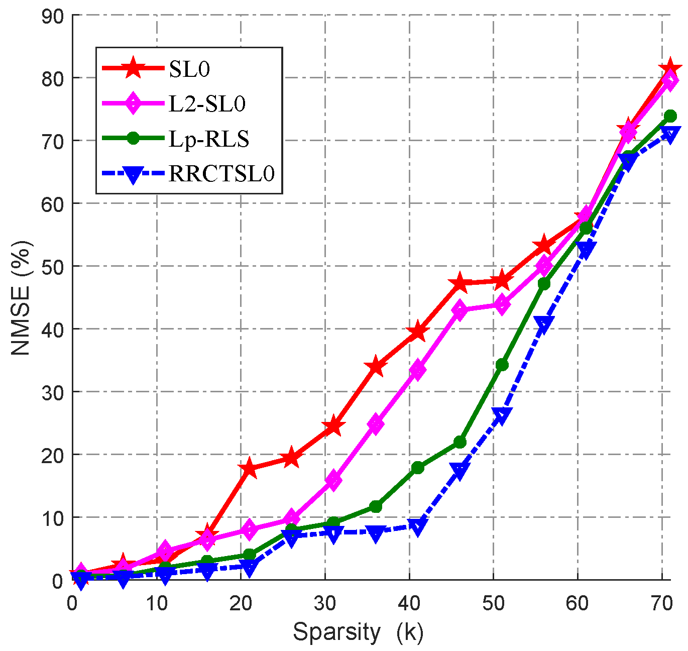
Figure 5 shows the NMSE with the increase of sparsity k. The reconstruction accuracy of these algorithms is inversely related to the value of NMSE. We can see that the RRCTSL0 always obtains the smallest NMSE with the increase of k. This indicates that the RRCTSL0 algorithm has the most accurate reconstruction performance.

From Figure 6, we can see that the larger the signal length is, the longer the CRT. We can see that the SL0 and $L_2$-SL0 algorithms perform better than the proposed RRCTSL0 algorithm, while the proposed RRCTSL0 algorithm outperforms the $L_p$-RLS algorithm. Therefore, improving reconstruction speed is one of the main directions of the RRCTSL0 algorithm in the future.

3.3. Applications of the Proposed RRCTSL0 Algorithm

3.3.1. Real Sparse Signal Recovery

Real signal recovery is a popular application of CS technology. Here, we applied the proposed RRCTSL0 algorithm to the reconstruction of a real combined signal. We fixed the length of signal at $n=256$, the number of measurement at $m=64$, and sparsity at $k=6$. Given $\{\mathit{y},\mathsf{\Phi },\mathit{b}\}$, we tried to recover combined signal $\tilde{\mathit{X}}=0.3cos\left(2\pi f_1{T}_s{\mathit{t}}_{\mathit{s}}\right)+0.6sin\left(2\pi f_2{T}_s{\mathit{t}}_{\mathit{s}}\right)+0.1cos\left(2\pi f_3{T}_s{\mathit{t}}_{\mathit{s}}\right)$, where $f_1=50,f_2=100,f_3=200$ are the signal frequency, $T_s=1/800$ is the sampling interval, and ${\mathit{t}}_{\mathit{s}}=[1,2,3,\cdots ,n]$ is the sampling sequence. The recovery process of combined signal $\tilde{\mathit{X}}$ is shown in Figure 7.

Figure 8 shows the recovery effect of real combined signal $\tilde{\mathit{X}}$ by the RRCTSL0 algorithm under different $\xi$. Meanwhile, the time-frequency characteristics (obtained by short-time Fourier transform) are shown in Figure 9. Obviously, when $\xi$ varies within the range of [0, 0.5], the recovery signal is very appropriate to $\tilde{\mathit{X}}$. This proves that the RRCTSL0 algorithm can accurately recover real sparse combined signal under certain noise.

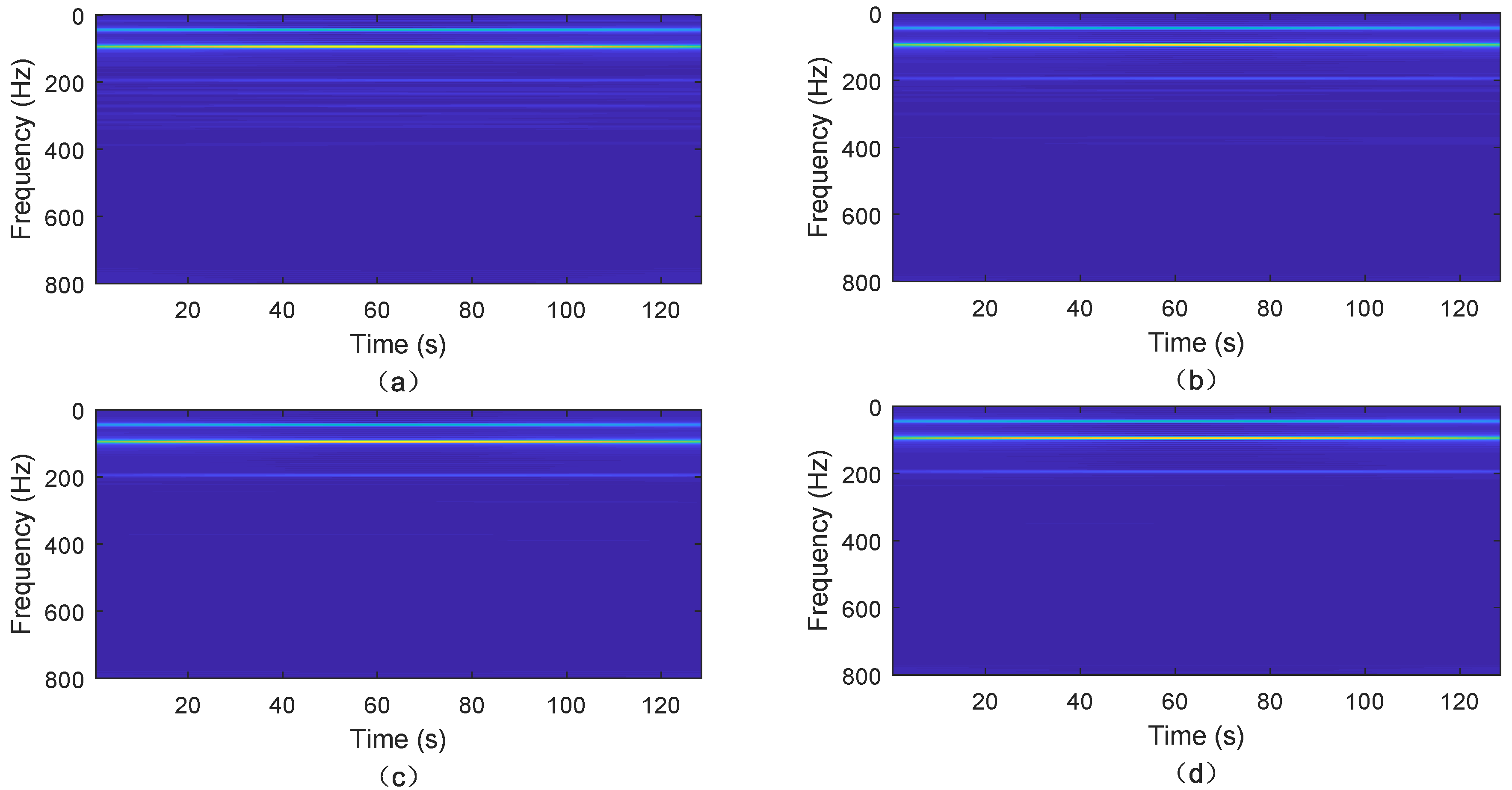
Figure 10 shows the recovery effect of real combined signal $\tilde{\mathit{X}}$ implemented by different algorithms under noise intensity $\xi =0.1$. Meanwhile, time-frequency characteristics (obtained by short-time Fourier transform) are shown in Figure 11. It can be seen that the RRCTSL0 algorithm performs better than the other three algorithms (the $L_p$-RLS algorithm performs very similarly to the proposed RRCTSL0 algorithm, but the RRCTSL0 algorithm performs better if carefully observed). The main reasons are: (1) The unconstrained regularization mechanism can globally optimize the $L_0$-norm, thus improving the antinoise performance of the RRCTSL0 in the optimization process. (2) The combination of the CT smoothed and new reweighted functions can promote signal sparsity. It is verified that the proposed RRCTSL0 algorithm has good practical value in sparse-signal recovery.

3.3.2. Real-Image Recovery

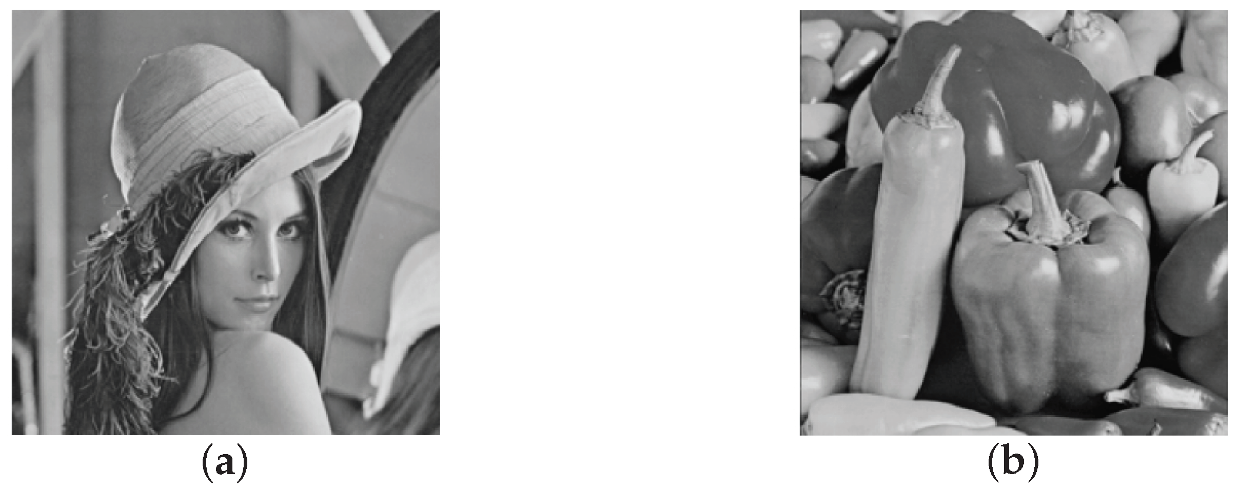
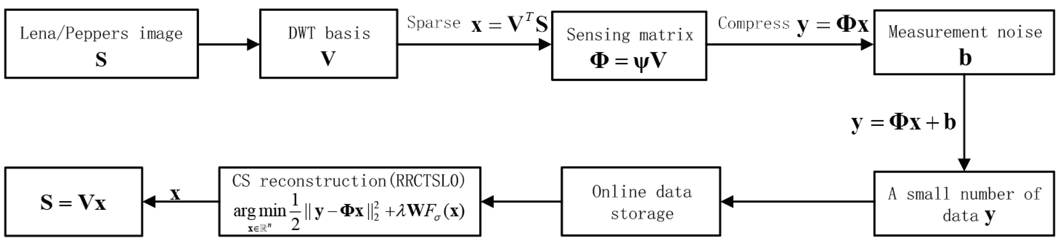
Real images are considered to be approximately sparse under a proper basis, such as the discrete cosine transform (DCT) basis and the discrete wavelet transform (DWT) basis. Here, we simulated the recovery performances of the proposed RRCTSL0 algorithm based on the two real images in Figure 12: Lena, Peppers. Specifically, in order to reveal sparse coefficients $\mathit{x}$ of real images $\mathit{s}$, we used DWT basis $\mathit{V}$: $\mathit{s}=\mathit{V}\mathit{x}$, and $\mathit{x}={\mathit{V}}^T\mathit{s}$. Noisy measurements $\mathit{y}$ were obtained as follows:

$$\mathit{y}=\mathbf{\psi }\mathit{s}+\mathit{b}=\mathbf{\psi }\mathit{V}\mathit{x}+\mathit{b}=\mathsf{\Phi }\mathit{x}+\mathit{b}.$$

(29)

The entries of measurement noise $\mathit{b}$ were generated using i.i.d. Gaussian distribution $\mathcal{N}(0,\xi )$. Taking the RRCTSL0 algorithm, we could solve this image-recovery problem as shown in Figure 13. Here, we used Peak SNR (PSNR) and a Structural Similarity Index (SSIM) to compare the recovery performance of different algorithms. PSNR is defined as

$$\mathrm{PSNR}=10log({255}^2/\mathrm{MSE}),$$

(30)

where $\mathrm{MSE}=\left|\right|\mathit{x}-\widehat{\mathit{x}}{\left|\right|}_2^2$; and SSIM is defined as

$$\mathrm{SSIM}(p,q)=\frac{(2{\mu }_p+{\mu }_q+c_1)(2{\sigma }_{pq}+c_2)}{({\mu }_p^2+{\mu }_q^2+c_1)({\sigma }_p^2+{\sigma }_q^2+c_2)}.$$

(31)

Among these, ${\mu }_p$ is the mean of image p, ${\mu }_q$ is the mean of image q, ${\sigma }_p$ is the variance of image p, ${\sigma }_q$ is the variance of image q, and ${\sigma }_{pq}$ is covariance between image p and image q. Parameters $c_1=z_{1}L$ and $c_2=z_{2}L$, which $z_1=0.01,z_2=0.03$, and L is the dynamic range of the pixel values. The range of SSIM was $[-1,1]$ and, when these two images were the same, the SSIM equaled to 1.

Table 2. Peak SNR (PSNR) and Structural Similarity Index (SSIM) of the recovered Lena image by the SL0, $L_2$-SL0, and $L_p$-RLS algorithms and the proposed RRCTSL0 algorithm with $\xi =0.01$.

CR	PSNR (dB)				SSIM (%)
	SL0	${\mathit{L}}_2$-SL0	${\mathit{L}}_{\mathit{p}}$-RLS	RRCTSL0	SL0	${\mathit{L}}_2$-SL0	${\mathit{L}}_{\mathit{p}}$-RLS	RRCTSL0
0.4	29.075	29.255	32.369	34.825	98.24	98.28	99.16	99.53
0.5	30.379	30.688	34.664	36.669	98.70	98.77	99.51	99.69
0.6	33.140	30.232	36.699	36.789	99.31	98.64	99.69	99.70

and

Table 3. PSNR and SSIM of the recovered Peppers image by the SL0, $L_2$-SL0, and $L_p$-RLS algorithms and the proposed RRCTSL0 algorithm with $\xi =0.01$.

CR	PSNR (dB)				SSIM (%)
	SL0	L2-SL0	${\mathit{L}}_{\mathit{q}}$-RLS	RRCTSL0	SL0	L2-SL0	${\mathit{L}}_{\mathit{q}}$-RLS	RRCTSL0
0.4	21.811	26.343	33.887	34.673	93.13	97.33	99.53	99.61
0.5	28.405	29.769	34.588	35.046	98.35	98.80	99.60	99.64
0.6	32.276	33.188	34.872	35.160	99.33	99.45	99.63	99.65

show PSNR and SSIM recovered by different algorithms. We can see that the proposed RRCTSL0 algorithm always showed the best performance in terms of PSNR and SSIM at compression ratio (CR) $\in [0.4,0.5,0.6]$, where CR is defined as $m/n$.

Then, we fixed CR to 0.5, and analyzed the image-recovery effects of the RRCTSL0 algorithm at $\xi$ = [0, 0.05, 0.1, 0.2, 0.5], as shown in Figure 14 and Figure 15. Moreover, we show the PSNR and SSIM in detail by scientific data in

Table 4. PSNR and SSIM of the recovery image by the proposed RRCTSL0 algorithm when noise was incrementing according to sequence $\xi =[0,0.05,0.1,0.2,0.5]$.

$\mathit{\xi }$	Photo	PSNR (dB)	SSIM (%)
0	Lena	38.492	99.80
	Peppers	39.367	99.87
0.05	Lena	29.203	98.28
	Peppers	28.826	97.53
0.1	Lena	24.272	94.78
	Peppers	24.305	95.64
0.2	Lena	18.727	83.43
	Peppers	19.782	86.07
0.5	Lena	12.489	49.50
	Peppers	13.416	55.34

. From Figure 14 and Figure 15, and Table 4, we can see that the RRCTSL0 algorithm performs well when $\xi$ is less than 0.2. However, when $\xi$ is over 0.2, the image-recovery effects of the RRCTSL0 algorithm significantly reduce. These show that the proposed RRCTSL0 has a certain ability to denoise, but under high noise conditions, the effect needs to be improved.

4. Conclusions

In this paper, we proposed the RRCTSL0 algorithm, which can be used for finding sparse solutions for an USLE. We proved that the RRCTSL0 algorithm is an effective method for recovering sparse signals and images. In the RRCTSL0 algorithm, the symmetric CT function is used as a DA function to approximate an $L_0$-norm, and the reweighted function is combined with the CT function to promote sparsity. Simultaneously, the objective optimization model was established with an unconstrained regularization mechanism. Based on this, the RRCTSL0 algorithm performs the optimization process with the CG method to obtain an optimal solution. Experiments on both simulated and real data showed that the RRCTSL0: (1) had faster convergence speed; (2) could improve reconstruction accuracy and had better denoise performance; (3) satisfied the needs of sparse-signal and image recovery. In addition, improving the ability of the RRCTSL0 algorithm to resist non-Gaussian noise would be our future work. Moreover, we would also like to apply the RRCTSL0 algorithm to other compressive sensing applications, such as SAR imaging [36], hyperspectral image classification [37], magnetic resonance imaging (MRI) [38], electrocardiograms (ECG) [39], and transfer hashing [40].

References

- Donoho, D.L. Compressed sensing. IEEE Trans. Inf. Theory 2006, 52, 1289–1306. [Google Scholar] [CrossRef]
- Cand’es, E.J.; Wakin, M.B. An introduction to compressive sampling. IEEE Signal Process. Mag. 2008, 2, 21–30. [Google Scholar] [CrossRef]
- Badeńska, A.; Błaszczyk, L. Compressed sensing for real measurements of quaternion signals. J. Frankl. Inst. 2017, 354, 5753–5769. [Google Scholar] [CrossRef] [Green Version]
- Routray, S.; Ray, A.K.; Mishra, C. MRI Denoising Using Sparse Based Curvelet Transform with Variance Stabilizing Transformation Framework. Indones. J. Electr. Eng. Comput. Sci. 2017, 7, 116–122. [Google Scholar]
- Luan, S.; Zhang, B.; Zhou, S.; Chen, C.; Han, J.; Yang, W. Gabor convolutional networks. IEEE Trans. Image Process. 2018, 27, 4357–4366. [Google Scholar] [CrossRef] [PubMed]
- Huang, S.; Tran, T.D. Sparse Signal Recovery via Generalized Entropy Functions Minimization. arxiv, 2017; arXiv:1703.10556. [Google Scholar]
- Tropp, J.A.; Gilbert, A.C. Signal recovery from random measurements via orthogonal matching pursuit. IEEE Trans. Inf. Theory 2007, 12, 4655–4666. [Google Scholar] [CrossRef]
- Wen, J.; Zhou, Z.; Wang, J.; Tang, X.; Mo, Q. A sharp condition for exact support recovery with orthogonal matching pursuit. IEEE Trans. Signal Process. 2017, 6, 1370–1382. [Google Scholar] [CrossRef]
- Jian, W.; Seokbeop, K.; Byonghyo, S. Generalized orthogonal matching pursuit. IEEE Trans. Signal Process. 2012, 12, 6202–6216. [Google Scholar] [CrossRef]
- Wang, J.; Kwon, S.; Li, P.; Shim, B. Recovery of sparse signals via generalized orthogonal matching pursuit: A new analysis. IEEE Trans. Signal Process. 2016, 4, 1076–1089. [Google Scholar] [CrossRef]
- Needell, D.; Tropp, J.A. CoSaMP: Iterative signal recovery from incomplete and inaccurate samples. Commun. ACM 2010, 12, 93–100. [Google Scholar] [CrossRef]
- Dai, W.; Milenkovic, O. Subspace pursuit for compressive sensing signal reconstruction. IEEE Trans. Inf. Theory 2009, 5, 2230–2249. [Google Scholar] [CrossRef]
- Liu, J.; Zhang, C.; Pan, C. Priori-information hold subspace pursuit: A compressive sensing-based channel estimation for layer modulated tds-ofdm. IEEE Trans. Broadcast. 2018, 99, 1–9. [Google Scholar] [CrossRef]
- Ekanadham, C.; Tranchina, D.; Simoncelli, E.P. Recovery of Sparse Translation-Invariant Signals with Continuous Basis Pursuit. IEEE Trans. Signal Process. 2011, 10, 4735–4744. [Google Scholar] [CrossRef] [PubMed]
- Goldstein, T.; Studer, C. Phasemax: Convex phase retrieval via basis pursuit. IEEE Trans. Inf. Theory 2018, 4, 2675–2689. [Google Scholar] [CrossRef]
- Khan, S.U.; Qureshi, I.M.; Haider, H.; Zaman, F.; Shoaib, B. Diagnosis of faulty sensors in phased array radar using compressed sensing and hybrid IRLS–SSF algorithm. Wirel. Pers. Commun. 2016, 91, 1–20. [Google Scholar] [CrossRef]
- Zhao, R.; Lai, X.; Hong, X.; Lin, Z. A matrix-based IRLS algorithm for the least Lp-norm design of 2-d fir filters. Multidimens. Syst. Signal Process. 2017, 2, 1–15. [Google Scholar]
- Ewald, K.; Schneider, U. Uniformly valid confidence sets based on the lasso. Statistics 2018, 12, 1358–1387. [Google Scholar] [CrossRef]
- Wright, S.J.; Nowak, R.D.; Figueiredo, M.A.T. Sparse reconstruction by separable approximation. IEEE Trans. Signal Process. 2009, 7, 2479–2493. [Google Scholar] [CrossRef]
- Qiao, B.; Zhang, X.; Wang, C.; Zhang, H.; Chen, X. Sparse regularization for force identification using dictionaries. J. Sound Vib. 2016, 368, 71–86. [Google Scholar] [CrossRef]
- Ye, X.; Zhu, W.; Zhang, A.; Meng, Q. Sparse channel estimation in MIMO-OFDM systems based on an improved sparse reconstruction by separable approximation algorithm. J. Inf. Comput. Sci. 2013, 10, 609–619. [Google Scholar]
- Quan, X.; Zhang, B.; Wang, Z.; Gao, C.; Yirong, W.U. An efficient data compression technique based on BPDN for scattered fields from complex targets. Sci. China (Inf. Sci.) 2017, 60, 109302. [Google Scholar] [CrossRef]
- Li, Z.X.; Li, Z.C. Accelerated 3D blind separation of convolved mixtures based on the fast iterative shrinkage thresholding algorithm for adaptive multiple subtraction. Geophysics 2018, 83, V99–V113. [Google Scholar] [CrossRef]
- Kim, D.; Fessler, J.A. Another look at the fast iterative shrinkage/thresholding algorithm (FISTA). Siam J. Optim. 2018, 28, 223–250. [Google Scholar] [CrossRef] [PubMed]
- Pant, J.K.; Lu, W.S.; Antoniou, A. New Improved Algorithms for Compressive Sensing Based on ℓp Norm. IEEE Trans. Circuits Syst. II Express Briefs 2014, 61, 198–202. [Google Scholar] [CrossRef]
- Ye, X.; Zhu, W.P.; Zhang, A.; Yan, J. Sparse channel estimation of MIMO-OFDM systems with unconstrained smoothed L0-norm-regularized least squares compressed sensing. Eurasip J. Wirel. Commun. Netw. 2013, 2013, 282. [Google Scholar] [CrossRef]
- Mohimani, H.; Babaie-Zadeh, M.; Jutten, C. A Fast Approach for Overcomplete Sparse Decomposition Based on Smoothed ℓ0 Norm. IEEE Trans. Signal Process. 2009, 57, 289–301. [Google Scholar] [CrossRef]
- Malek-Mohammadi, M.; Koochakzadeh, A.; Babaie-Zadeh, M.; Jansson, M.; Rojas, C.R. Successive concave sparsity approximation for compressed sensing. IEEE Trans. Signal Process. 2016, 64, 5657–5671. [Google Scholar] [CrossRef]
- Guo, Q.; Ruan, G.; Liao, Y. A time-frequency domain underdetermined blind source separation algorithm for mimo radar signals. Symmetry 2017, 9, 104. [Google Scholar] [CrossRef]
- Candès, E.J.; Wakin, M.B.; Boyd, S.P. Enhancing sparsity by reweighted L1 minimization. J. Fourier Anal. Appl. 2008, 14, 877–905. [Google Scholar] [CrossRef]
- Shi, Z. A Weighted Block Dictionary Learning Algorithm for Classification. Math. Probl. Eng. 2016, 2016, 1–15. [Google Scholar] [CrossRef]
- Fang, X.F.; Zhang, J.S.; Li, Y.Q. Sparse Signal Reconstruction Based on Multiparameter Approximation Function with Smoothed Norm. Math. Probl. Eng. 2014, 6, 1–9. [Google Scholar]
- Wang, J.H.; Huang, Z.T.; Zhou, Y.Y.; Wang, F.H. Robust sparse recovery based on approximate l0 norm. Acta Electron. Sin. 2012, 40, 1185–1189. [Google Scholar]
- Xiao, J.; Del-Blanco, C.R.; Cuevas, C.; García, N. Fast image decoding for block compressed sensing based encoding by using a modified smooth l0-norm. In Proceedings of the International Conference on Consumer Electronics, Berlin, Germany, 5–7 September 2016; pp. 242–244. [Google Scholar]
- Ye, X.; Zhu, W.P. Sparse channel estimation of pulse-shaping multiple-input–multiple-output orthogonal frequency division multiplexing systems with an approximate gradient L2-SL0 reconstruction algorithm. Iet Commun. 2014, 8, 1124–1131. [Google Scholar] [CrossRef]
- Tian, H.; Li, D. Sparse flight array SAR downward-looking 3-d imaging based on compressed sensing. IEEE Geosci. Remote Sens. Lett. 2016, 13, 1395–1399. [Google Scholar] [CrossRef]
- Li, H.; Li, C.; Zhang, C.; Liu, Z.; Liu, C. Hyperspectral image classification with spatial filtering and ℓ2,1 norm. Sensors 2017, 17, 314. [Google Scholar] [CrossRef]
- Lazarus, C.; Weiss, P.; Vignaud, A.; Ciuciu, P. An empirical study of the maximum degree of undersampling in compressed sensing for T2*-weighted MRI. Magn. Reson. Imaging 2018, 53, 112–122. [Google Scholar] [CrossRef] [PubMed]
- Tseng, Y.H.; Chen, Y.H.; Lu, C.W. Adaptive integration of the compressed algorithm of CS and NPC for the ECG signal compressed algorithm in VLSI implementation. Sensors 2017, 17, 2288. [Google Scholar] [CrossRef] [PubMed]
- Zhou, J.T.; Zhao, H.; Peng, X.; Fang, M.; Qin, Z.; Goh, R.S.M. Transfer hashing: From shallow to deep. IEEE Trans. Neural Netw. Learn. Syst. 2018, 99, 1–11. [Google Scholar] [CrossRef] [PubMed]
Figure 1.
Framework of a compressive sensing (CS) model with noise.
Figure 2.
Different delta-approximating (DA) functions are plotted in this figure for , , displaying the -norm and -norm of 2D.
Figure 3.
Normalized mean square error (NMSE) of recovery signal changes with iterations. (a) Comparison between SL0, -SL0, -RLS algorithms and the proposed RRCTSL0 algorithm; (b) effect of the RRCTSL0 algorithm under sparsity .
Figure 4.
Signal-to-noise ratio (SNR) analysis. (a) Signal SNR for the SL0, -SL0, -RLS algorithms and the proposed RRCTSL0 algorithm with noise intensity from 0 to 0.5 (the interval is 0.05) during 100 runs; (b) SNR for proposed RRCTSL0 algorithm with while .
Figure 5.
Signal NMSE analysis for the SL0, -SL0, -RLS algorithms and the proposed RRCTSL0 algorithm with sparsity k from 1 to 71 at an interval of 5, during 100 runs in the noise case .
Figure 6.
Signal CPU running time (CRT) analysis for the SL0, -SL0, -RLS algorithms and the proposed RRCTSL0 algorithm with the length of signal n equaling [170, 220, 270, 320, 370, 420, 470, 520], during 100 runs in noise case .
Figure 7.
Recovery process of the combined signal by the RRCTSL0 algorithm.
Figure 8.
Signal-recovery effect by proposed RRCTSL0 algorithm when noise is incrementing according to sequence = [0, 0.05, 0.1, 0.2, 0.5]. (a) = 0; (b) = 0.05; (c) = 0.1; (d) = 0.2; (e) = 0.5.
Figure 9.
Reconstruction time-frequency characteristics of the proposed RRCTSL0 algorithm when noise is incrementing according to sequence = [0, 0.05, 0.1, 0.2, 0.5]. (a) Time-frequency characteristic of the original signal; (b) = 0; (c) = 0.05; (d) = 0.1; (e) = 0.2; (f) = 0.5.
Figure 10.
Signal recovery effect by different algorithms when . (a) Signal recovery by the SL0 algorithm; (b) signal recovery by the -SL0 algorithm; (c) signal recovery by the -RLS algorithm; (d) signal recovery by the RRCTSL0 algorithm.
Figure 11.
Reconstruction time-frequency characteristics of different algorithms when . (a) SL0; (b) -SL0; (c) -RLS; (d) RRCTSL0.
Figure 12.
Real images used in the recovery experiments: (a) Lena (); (b) Peppers ().
Figure 13.
Recovery process of the real images by the RRCTSL0 algorithm.
Figure 14.
Lena image-recovery effect by the proposed RRCTSL0 algorithm when noise was incrementing according to sequence = [0, 0.05, 0.1, 0.2, 0.5]. (a) = 0; (b) = 0.05; (c) = 0.1; (d) = 0.2; (e) = 0.5.
Figure 15.
Peppers image-recovery effect by the proposed RRCTSL0 algorithm when noise was incrementing according to sequence = [0, 0.05, 0.1, 0.2, 0.5]. (a) = 0; (b) = 0.05; (c) = 0.1; (d) = 0.2; (e) = 0.5.