m-Polar Fuzzy Soft Weighted Aggregation Operators and Their Applications in Group Decision-Making

Abstract

Aggregation operators are important tools for solving multi-attribute group decision-making (MAGDM) problems. The main challenging issue for aggregating data in a MAGDM problem is how to develop a symmetric aggregation operator expressing the decision makers’ behavior. In the literature, there are some methods dealing with this difficulty; however, they lack an effective approach for multi-polar inputs. In this study, a new aggregation operator for m-polar fuzzy soft sets (M-pFSMWM) reflecting different agreement scenarios within a group is presented to proceed MAGDM problems in which both attributes and experts have different weights. Moreover, some desirable properties of M-pFSMWM operator, such as idempotency, monotonicity, and commutativity (symmetric), that means being invariant under any permutation of the input arguments, are studied. Further, m-polar fuzzy soft induced ordered weighted average (M-pFSIOWA) operator and m-polar fuzzy soft induced ordered weighted geometric (M-pFSIOWG) operator, which are extensions of IOWA and IOWG operators, respectively, are developed. Two algorithms are also designed based on the proposed operators to find the final solution in MAGDM problems with weighted multi-polar fuzzy soft information. Finally, the efficiency of the proposed methods is illustrated by some numerical examples. The characteristic comparison of the proposed aggregation operators shows the M-pFSMWM operator is more adaptable for solving MAGDM problems in which different cases of agreement affect the final outcome.

1. Introduction

A group decision-making process, which is also called multi-person decision-making, is the problem of finding the best option accepted by the majority of decision makers among a list of possible alternatives. The basic act in the group decision-making is the process of consensus between different decision makers. Although a unanimous consensus is the ideal case, in real situations, full agreement rarely happens. Decision makers usually share and discuss their opinions about the alternatives to obtain a consensus or partial agreement for making the final decision. However, sometimes, they provide their priorities about the alternatives individually and then try to reach a consensus on them. Regardless which approach is applied, using aggregation operators is one of the most often used techniques to reach the process of consensus in group decision-making problems.

The aim of an aggregation operator of dimension K is to aggregate the K-tuple of objects into a single object by a bounded non-decreasing function $A:{\bigcup }_{K\in \mathbb{N}}{[0,1]}^K\to [0,1]$. The mean value, the median, the minimum, the maximum, the t-norms, and the t-conorms are commonly used to reach the process of consensus in group decision-making problems. To aggregate a sequence of inputs with different importance degrees, the concept of weighting vector in aggregation operators has been studied, such as the weighted minimum and the weighted maximum [1,2,3]; ordered weighted average (OWA) [4], which is calculated based on the arithmetic mean; and ordered weighted geometric (OWG) [5], which is formulated based on the geometric mean. The main disadvantage of OWA and OWG operators, i.e., ignoring the importance of given arguments $x_1,\cdots ,x_K$ for calculating the aggregated value, leads to definition of their extensions into the induced OWA (IOWA) operator [6], and induced OWG (IOWG) operator [7], respectively. However, these extensions have the inherent limitations from OWA operator and OWG operator, concerning the determination of associated weighting vector $\mathit{w}$ for IOWA and IOWG operators. In practice, there is no unique strategy to find the associated weighting vector $\mathit{w}$. Usually, a quantifier function $Q:[0,1]\to [0,1]$ whose definition may change from one case to another one is applied to compute the associated weighting vector $\mathit{w}={(w_1,\cdots ,w_K)}^T$ based on the formulation $w_i=Q(\frac{i}{K})-Q(\frac{i-1}{K})$ for all i [4,5,8,9].

Soft set theory (SS) [10], characterized by a set-valued function $f:P\to 2^U$, is defined by a parameterization family of the universe U. Thus, in comparison with fuzzy set theory [11], it allows us to have a more comprehensive description of U based on any type and number of parameters $p\in P$. The concepts of fuzzy soft set (FSS) [12] and intuitionistic fuzzy soft set (IFSS) [13] were also studied to handle more complicated problems. Although soft set theory was originally developed to cope with the lack of parameterization tool in fuzzy sets, its flexibility to deal with set-valued functions makes it a powerful tool for providing a new methodology in decision-making problems. The first adaptivity of soft sets in decision-making was conducted by Maji et al. [14]. However, they did not discuss the aggregation methods. Roy and Maji [15] gave an algorithm to solve a group decision-making problem based on fuzzy soft sets. The FS minimum operator was applied for finding the consensus of multi-source parameter sets. Later, Alcantud [16] overcame the disadvantages of Roy and Maji’s algorithm by applying FS product operator rather than FS minimum operator. Cagman et al. [17,18] applied FS minimum operator, FS maximum operator, and FS product operator to produce different fuzzy soft aggregation operators in a MAGDM problem. Guan et al. [19] applied the FS intersection operator for aggregating data. Then, a new ranking system of objects, in which the rate of objects is computed based on the full unanimity of experts with respect to all parameters rather than the number of parameters that are owned by each object, was constructed to rank alternatives in a group decision problem. Zhang et al. [20] used the IFS maximum operator to check the process of consensus in MAGDM problem. Mao et al. [21] extended IFSOWA and IFSOWG operators for intuitionistic fuzzy soft sets under three different cases of experts’ weights called completely known, partly known, and completely unknown. Das and Kar [22] used the IFS product and the IFS sum operators of intuitionistic fuzzy soft matrices to obtain a collective opinion among different decision makers. Zhang and Zhang [23] utilized the FS union operation to reach the process of consensus in MAGDM problems based on trapezoidal interval type-2 fuzzy soft sets (TIT2FSSs). The TOPSIS approach was then applied to select the best option. However, recently, Pandey and Kumar [24] modified this procedure so that the complement operation that is used by Zhang and Zhang can only be applied for TIT2FSSs in which left and right heights are equal. Tao et al. [25] proposed four aggregation functions, including the soft maximum operator, soft minimum operator, soft average operator, and soft weighted average operator, to aggregate data in MAGDM problems. Two selection tools based on the SAW method and comparison matrix were also developed to obtain the optimal decision. Zhu and Zhan [26] developed the new concept fuzzy parameterized fuzzy soft sets (FPFSS), where the parameters are considered as fuzzy sets and then the consensus stage proceeds by using the t-norm and t-conorm products of FPFSSs. A new choice value function is also introduced to handle the process of selection. On the other hand, some researchers attempted to develop novel aggregation methods for FSS and IFSS. For example, Zahedi et al. [27,28] extended the concept of fuzzy soft topology to reach the consensus based on a collective preorder relation.

Conventionally, soft-set-based aggregating tools have been developed for unipolar input data where the truth value belongs to $[0,1]$. Some situations require multi-polar arguments to be aggregated. To handle the problem of multi-polarity in consensus process, some studies extended the aggregation operators from unipolar scale into the bipolar scale (i.e., the interval $[-1,1]$) [29] and multi-polar scale (i.e., the space $K\times [0,1]$ where K is a set of m different categories) [30,31]. These extensions allow dealing with inputs from different categories where the output is presented by a pair $(k,x)$ that k shows the category of aggregated value x. However, in many decision-making problems, the attribute set contains multi-feature or multi-polar decision parameters where the final decision should reflect the best option based on all multi-polar attributes beyond their category. For example, in the hotel booking problem, “Location” is one of the most important parameters for finding a good hotel to stay, which is a multi-feature parameter depending on how close it is to the main road, city center, tourist attractions, etc. A hotel is selected if it has the best location in terms of all features from different categories not only one. In fact, there is no ideal category k in final solution. This issue becomes more complex when a group of people want to choose a hotel. In this case, different cases of agreement within a group including unanimous consensus and partial agreement, e.g., “almost all”, “most”, and “more than 50%”, are considered to obtain the collective view based on individuals’ opinions. Thus, an alternative aggregation operator is required to deal with multi-polar fuzzy attributes in group decision-making.

In a group decision process with multi-polar inputs, the performance of alternatives are judged by each decision maker with respect to each criterion. The main problem is to compare these judgements and reach a consensus among them. The existing aggregation methods usually consider weighted or unweighted cases under a unanimous agreement [15,16,17,18,19,20,21,22,23]. However, besides the importance degrees of experts, the consensus degree for a fuzzy majority of the experts and different choices of experts’ judgments at a consensus level should be taken into account in the proposed alternative aggregation operator to reach more reliable methodology. Moreover, due to the extreme applicability of FSSs in MAGDM problems with multi-polar fuzzy soft input information, adaptability of the proposed aggregation operator for m-polar fuzzy soft sets should be studied. To do this, an extension of fuzzy soft sets into the m-polar fuzzy soft sets, where the values of membership functions $f_p$ are extended from the unit interval $[0,1]$ into the cubic ${[0,1]}^m$, needs to be developed.

Until now, weighted aggregation operators for multi-polar fuzzy soft arguments have not been considered. Thus, this study was carried out to develop some weighted m-polar aggregation operators which cover different scenarios at the consensus degree for a fuzzy majority expressed by linguistic variables, such as “most”, “much more than 70%”, and “more than half”. The main goal is to design FS-set-based algorithms for finding the best solution in group decision-making with weighted multi-polar input information according to the proposed aggregation methods. To achieve this goal, the following problems are addressed in this study: (i) how to express the multi-polarity of input data under fuzzy soft environment; (ii) how to generate an aggregation method based on the fuzzy majority concept for weighted multi-polar inputs; (iii) how to apply the proposed aggregation method for finding the solution in group decision-making problems; and (iv) how to analyze the final result obtained by the proposed algorithm. Accordingly, there are four main contributions of this research as follows: (i) to define a new concept m-polar fuzzy soft set; (ii) to introduce m-polar fuzzy soft weighted aggregation operators based on the fuzzy majority concept; (iii) to design m-polar FS-based algorithms for finding the solution in group decision-making; and (iv) to give some illustrative examples for validating and comparing the results.

The rest of this paper is organized as the following. Section 2 represents some basic definitions and concepts from the related works. Section 3 gives a new aggregation operator, called M-pFSMWM, for weighted m-polar fuzzy soft data. This new procedure aggregates the experts’ judgments based on their importance degrees, a linguistic or numerical consensus level between the experts, and different choices of experts’ judgments at the consensus level. Some of its desirable properties as well as special families of M-pFSMWM operator according to different values of consensus degree $\alpha$ and weighting vector $\omega$ are studied. In Section 4, a new score value function is developed to design an algorithm for ranking alternatives in MAGDM problems based on the M-pFSMWM operator and a new m-polar fuzzy soft preference relation. To compare the proposed M-pFSMWM operator with some existing aggregation methodologies, in Section 5, the m-polar fuzzy soft induced ordered weighted average (M-pFSIOWA) operator and the m-polar fuzzy soft induced ordered weighted geometric (M-pFSIOWG) operator, which are the extensions of IOWA and IOWG operators, respectively, are developed and their properties are considered. We also present an algorithm to solve MAGDM problems based on M-pFSIOWA and M-pFSIOWG operators. Section 6 focuses on the efficiency of proposed techniques by some numerical examples. Finally, in Section 7, we discuss the advantages and limitations of our approach.

2. Preliminaries

This section recalls some definitions about the weighted aggregation operators, m-polar fuzzy sets, and fuzzy soft sets to achieve our main aim, proposing new algorithms for solving group decision-making based on alternative m-polar fuzzy soft aggregation operators, in the next sections.

2.1. Weighted Aggregation Operator

The weighted minimum and the weighted maximum are two important aggregation operators dealing with objects having non-negative weights ${\omega }_1,\cdots ,{\omega }_K$ such that ${\sum }_{i=1}^K{\omega }_i=1$. However, there is no unique solution to formulate them. For instance, Fagin and Wimmers [2] introduced the below formula to obtain the weighted minimum and the weighted maximum, respectively.

$$\begin{array}{c}\hfill {min}_{{\omega }_1,\cdots ,{\omega }_K}^{\otimes }(x_1,\cdots ,x_K)=\sum _{i=1}^K\left[i·({\omega }_{\sigma (i)}-{\omega }_{\sigma (i+1)})·min(x_{\sigma (1)},\cdots ,x_{\sigma (i)})\right]\end{array}$$

(1)

$$\begin{array}{c}\hfill {max}_{{\omega }_1,\cdots ,{\omega }_K}^{\otimes }(x_1,\cdots ,x_K)=\sum _{i=1}^K\left[i·({\omega }_{\sigma (i)}-{\omega }_{\sigma (i+1)})·max(x_{\sigma (1)},\cdots ,x_{\sigma (i)})\right]\end{array}$$

(2)

where $\sigma$ is a permutation that orders the weights as follows: ${\omega }_{\sigma (1)}\ge {\omega }_{\sigma (2)}\ge \cdots \ge {\omega }_{\sigma (K)}$ and ${\omega }_{\sigma (k+1)}=0$.

The IOWA operator, introduced by Yager and Filev [6], and the IOWG operator, given by Xu and Da [7], are also some commonly used tools for aggregating weighted objects. The IOWA operator is defined by

$$\begin{array}{c}\hfill IOWA(\langle {\omega }_1,x_1\rangle ,\cdots ,\langle {\omega }_K,x_K\rangle )=\sum _{j=1}^K{w}_j·y_j\end{array}$$

(3)

where $y_j$ is the value of $x_i$ that has the jth largest ${\omega }_i$ and ${\omega }_i$ in $\langle {\omega }_i,x_i\rangle$ is referred to as the order inducing variable and $x_i$ as the argument variable. The weights $w_1,\cdots ,w_K$ such that ${\sum }_{i=1}^K{\omega }_i=1$ are the associated weights to the IOWA operator that can be defined by a quantifier function $Q:[0,1]\to [0,1]$. Here, the re-ordering step of $x_i$s is carried out by the variable ${\omega }_i$ rather than the value of $x_i$, that is used to handle the re-ordering step in OWA operator, i.e., the collection $x_1,\cdots ,x_K$ is re-ordered as $\langle max\left\{{\omega }_i\right\},y_1\rangle \ge \cdots \ge \langle min\left\{{\omega }_i\right\},y_K\rangle$.

An IOWG operator is defined by

$$\begin{array}{c}\hfill IOWG(\langle {\omega }_1,x_1\rangle ,\cdots ,\langle {\omega }_K,x_K\rangle )=\prod _{j=1}^K{y_j}^{w_j}\end{array}$$

(4)

where $y_j$ is the value of $x_i$ that has the jth largest ${\omega }_i$ and ${\omega }_i$ in $\langle {\omega }_i,x_i\rangle$ is referred to as the order inducing variable and $x_i$ as the argument variable. Note that here also the re-ordering step is based on the inducing variable ${\omega }_i$ and weights $w_1,\cdots ,w_K$ such that ${\sum }_{i=1}^K{\omega }_i=1$ are the associated weights to the IOWG operator.

2.2. Fuzzy Sets

Today, fuzzy sets are known as an effective tool for modeling vague data [32,33,34,35]. If U is a non-empty set of elements, then a fuzzy subset X of U is a set of ordered pairs $(u,{\mu }_X(u))$ such that $u\in U$ and ${\mu }_X:U\to [0,1]$ is a membership function where ${\mu }_X(u)$ shows the membership degree of element u in X. Any fuzzy set R in $U\times U$ is called a fuzzy relation on U. If R represents a fuzzy preference relation on U, then, for each pair $(u,v)\in U\times U$, the value ${\mu }_R(u,v)$ shows the preference degree of u over v. Here, ${\mu }_R(u,v)=0.5$ indicates indifference between u and v ($u\sim v$), while ${\mu }_R(u,v)\in (0.5,1]$ shows u is preferred to v ($u\succ v$). Moreover, generally, we have ${\mu }_R(u,v)+{\mu }_R(v,u)=1$.

Theorem 1 (Multiplicative transitivity).

[36] If $u(.)$ is a utility function on the set $X=\{x_1,\cdots ,x_n\}$ such that the value $u(x_i)=u_i$ shows the utility of alternative $x_i\in X$, then the fuzzy preference relation R defined by ${\mu }_R(x_i,x_j)=r_{ij}=\frac{u_i}{u_i+u_j}$, which is a fuzzy preference relation satisfying multiplicative transitivity condition, i.e., $\frac{r_{ji}}{r_{ij}}\frac{r_{kj}}{r_{jk}}=\frac{r_{ki}}{r_{ik}}$ for all $i,j,k\in \{1,\cdots ,n\}$.

To extend the traditional fuzzy sets dealing with unipolar data into the multi-polar information, the concept of m-polar fuzzy set is defined as below.

Definition 1 (m-polar fuzzy set).

[37] An m-polar fuzzy set (M-pFS) X on U is a mapping $\mu :U\to {[0,1]}^m$, where ${[0,1]}^m$ refers to as the multiplication of $[0,1]\times \cdots \times [0,1]$ m-times, such that $\mu (u)=\left(({\mu }^1(u),\cdots ,{\mu }^m(u)\right)$, $\mathbf{0}=(0,0,\cdots ,0)$ and $\mathbf{1}=(1,1,\cdots ,1)$ are the least and greatest elements, respectively, and ${\mu }^c(u)=(1-{\mu }^1(u),\cdots ,1-{\mu }^m(u))$ shows its complement. The set of all m-polar fuzzy sets over U is represented by $m(U)$.

If ${\left\{{\mu }_k\right\}}_k$ is a family of M-pFSs over the universe U, then for any $u\in U$:

• If ${\mu }_i^s(u)\le {\mu }_j^s(u)$ for all $s=1,\cdots ,m$, then ${\mu }_i\le {\mu }_j$.
• $({\bigvee }_k{\mu }_k)(u)={sup}_k\left\{{\mu }_k(u)\right\}=({sup}_k\left\{{\mu }_k^1(u)\right\},\cdots ,{sup}_k\left\{{\mu }_k^m(u)\right\})$.
• $({\bigwedge }_k{\mu }_k)(u)={inf}_k\left\{{\mu }_k(u)\right\}=({inf}_k\left\{{\mu }_k^1(u)\right\},\cdots ,{inf}_k\left\{{\mu }_k^m(u)\right\})$.

2.3. Fuzzy Soft Sets

Theory of soft sets is presented based on the approximate descriptions of the set U. A soft set is characterized by a set-valued mapping $f:P\to 2^U$ where P is a set of parameters and $2^U$ shows the power set of U. By combining the definitions of fuzzy sets and soft sets a new concept called fuzzy soft set is proposed.

Definition 2 (Fuzzy soft set).

[12] A fuzzy soft set (FSS), denoted by $f_P$ or $(f,P)$, is a mapping $f:P\to {[0,1]}^U$ where for every $p\in P$, $f(p)$ is a fuzzy subset of U with membership function $f_p:U\to [0,1]$ where $\tilde{\mathbf{0}}$ and $\tilde{\mathbf{1}}$, defined by $\tilde{\mathbf{0}}(p)(u)=0$ and $\tilde{\mathbf{1}}(p)(u)=1$ $\forall u\in U$ and $p\in P$, is called the null fuzzy soft set and the absolute fuzzy soft set, respectively. Moreover, the complement of $(f,P)$, denoted by $(f^c,P)$, is defined by $f^c:P\to {[0,1]}^U$ where $\forall p\in P$, $f_p^c(u)=1-f_p(u)$ for all $u\in U$.

If ${\left\{(f_k,P_k)\right\}}_k$ is a family of FSSs over the universe U, then, for any $u\in U$:

• If $P_i\subset P_j$ and $f_i(p)(u)\le f_j(p)(u)$ for all $p\in P_i$, then $(f_i,P_i)\tilde{\le }(f_j,P_j)$.
• $({\tilde{\vee }}_k{f}_k)(p)(u)={sup}_k\left\{f_k(p)(u)\right\}$ for all $p\in {\cup }_k{P}_k$.
• $({\tilde{\wedge }}_k{f}_k)(p)(u)={inf}_k\left\{f_k(p)(u)\right\}$ for all $p\in {\cap }_k{P}_i$.

3. A New Weighted Aggregation Operator for M-pFSSs

In this section, we introduce a new weighted aggregation operator, called M-pFSMWM operator, to improve the aggregating tools for multi-polar inputs with non-negative weights under fuzzy soft environment. The advantages of this new operator is also demonstrated by some theorems and properties. To this end, we first develop the new concept of m-polar fuzzy soft sets (M-pFSS) and then introduce the M-pFSMWM operator in the domain of m-polar fuzzy soft sets.

3.1. m-Polar Fuzzy Soft Sets

Motivated by m-polar fuzzy sets given in Definition 1, the notion of m-polar fuzzy soft set is developed to model data dealing with multi-polar or multi-feature attributes. Basic operations of m-polar fuzzy soft sets are also discussed in this section.

Definition 3 (m-polar fuzzy soft set).

Let U and P be two non-empty sets of alternatives and parameters, respectively. The pair $(f,P)$ where f is the mapping $f:P\to m(U)$ such that for any $p\in P$ the $f(p)$ is an m-polar fuzzy subset of U can be defined as an m-polar fuzzy soft set (M-pFSS) over U. It means, for each $p\in P$ and any $u\in U$, $f(p)(u)$ is an m-tuple $f_p(u)=(f_p^1(u),f_p^2(u),\cdots ,f_p^m(u))$ such that the $f_p^s(u)$, for $s=1,2,\cdots ,m$, represents the relation between object $u\in U$ and feature s of parameter p.

The set of all m-polar fuzzy soft sets is shown by $mfs(U)$. Furthermore, an m-polar fuzzy soft set $(f,P)$ is called a null M-pFSS, shown by $\tilde{\mathbf{0}}$, or an absolute M-pFSS, shown by $\tilde{\mathbf{1}}$, if for any $p\in P$, $f^s(p)(u)=0$ and $f^s(p)(u)=1$, respectively, for all $u\in U$ and $1\le s\le m$. The complement of M-pFSS $(f,P)$ is also an M-pFSS, shown by $(f^c,P)$, where for any $p\in P$ and $u\in U$: ${f^s}^c(p)(u)=1-f^s(p)(u)$ for all $s=1,2,\cdots ,m$.

Example 1.

Let us suppose a person wants to rate four restaurants $\{x_1,x_2,x_3,x_4\}$ according to the parameters $\{p_1=Location,p_2=Meal,p_3=Services\}$. Let he/she considers the different aspects of these parameters as follows: The location of the restaurants includes close to the main road, in green surroundings, and in shopping mall. The meal of the restaurants includes main course, appetizer (starter), and dessert. The services of the restaurants include parking lot, live music, and free Wi-Fi connectivity.

Assume that the person uses the linguistic variables “No” (0), “Yes” (1), “Very Poor” (0), “Poor” (0.1), “Medium Poor” (0.3), “Medium” (0.5), “Medium Good”(0.7), “Good” (0.9), “Very Good” (1) “Very Far” (0), “Far” (0.1), “Medium Far” (0.3), “Medium Close”(0.7), “Close” (0.9), and “Very Close” (1) shown in

Table 1. Linguistic variables for describing each alternative with respect to the parameters.

U		${\mathit{x}}_1$	${\mathit{x}}_2$	${\mathit{x}}_3$	${\mathit{x}}_4$
$p_1$:
	$p_1^1$	Close	Far	Very Far	Very Close
	$p_1^2$	No	No	Yes	Yes
	$p_1^3$	Yes	Yes	No	No
$p_2$:
	$p_2^1$	Very Good	Medium	Medium Poor	Good
	$p_2^2$	Very Poor	Good	Medium	Good
	$p_2^3$	Medium	Very Good	Poor	Medium
$p_3$:
	$p_3^1$	Yes	Yes	Yes	No
	$p_3^2$	No	Yes	Yes	Yes
	$p_3^3$	Medium Good	Medium	Poor	Good

for describing the performance of each alternative with respect to these parameters.

Thus, a three-polar fuzzy soft set (that is shown in

Table 2. Tabular representation of M-pFSS $(f,P)$.

U	${\mathit{p}}_1$	${\mathit{p}}_2$	${\mathit{p}}_3$
$x_1$	(0.9,0,1)	(1,0,0.5)	(1,0,0.7)
$x_2$	(0.1,0,1)	(0.5,0.9,1)	(1,1,0.5)
$x_3$	(0,1,0)	(0.3,0.5,0.1)	(1,1,0.1)
$x_4$	(1,1,0)	(0.9,0.9,0.5)	(0,1,0.9)

) can help he/she to explain his/her opinion about these four restaurants.

For example, if the person considers the meal of the restaurant $x_1$, then the 3-tuple (1,0,0.5) means that the main course of the restaurant $x_1$ is very good while the starter and the dessert are very poor and medium, respectively.

Definition 4.

Let ${\left\{(f_k,P_k)\right\}}_k$ be a family of M-pFSSs over the common universe U and parameter sets $P_k$. Then, for any $u\in U$:

1. 

$(f_i,P_j)\tilde{\le }(f_j,P_j)$ if $P_i\subseteq P_j$ and $f_i^s(a)(u)\le f_j^s(a)(u)$ for all $a\in P_i$ and $s=1,2,\cdots ,m$.

2. 

$({\tilde{\vee }}_k{f}_k)(a)(u)={sup}_k\left\{f_k(a)(u)\right\}=({sup}_k\left\{f_k^1(a)(u)\right\},\cdots ,{sup}_k\left\{f_k^m(a)(u)\right\})$, for all $a\in {\bigcup }_{k\in K}{P}_k$.

3. 

$({\tilde{\wedge }}_k{f}_k)(a)(u)={inf}_k\left\{f_k(a)(u)\right\}=({inf}_k\left\{f_k^1(a)(u)\right\},\cdots ,{inf}_k\left\{f_k^m(a)(u)\right\})$, for all $a\in {\bigcap }_{k\in K}{P}_k$.

Proposition 1.

Let U and F be the universal sets of objects and parameters, respectively, and $P,Q$, and E are some subsets of F. Assume that $(f,P),(g,Q)$, and $(h,E)$ are some m-polar fuzzy soft sets over U where $f_p,g_q,h_e\in m(U)$ for all $p\in P,q\in Q$, and $e\in E$. Then:

1. 

$(f,P)\tilde{\vee }\tilde{0}=(f,P)$, $(f,P)\tilde{\wedge }\tilde{0}=\tilde{0}$ and $(f,P)\tilde{\vee }\tilde{1}=\tilde{1}$ and $(f,P)\tilde{\wedge }\tilde{1}=(f,P)$.

2. 

(Idempotent) $(f,P)\tilde{\vee }(f,P)=(f,P)$ and $(f,P)\tilde{\wedge }(f,P)=(f,P)$.

3. 

(Commutative) $(f,P)\tilde{\vee }(g,Q)=(g,Q)\tilde{\vee }(f,P)$ and $(f,P)\tilde{\wedge }(g,Q)=(g,Q)\tilde{\wedge }(f,P)$.

4. 

(Associative) $(f,P)\tilde{\vee }\left[(g,Q)\tilde{\vee }(h,E)\right]=\left[(f,P)\tilde{\vee }(g,Q)\right]\tilde{\vee }(h,E)$ and

$(f,P)\tilde{\wedge }\left[(g,Q)\tilde{\wedge }(h,E)\right]=\left[(f,P)\tilde{\wedge }(g,Q)\right]\tilde{\wedge }(h,E)$.

5. 

(Distributive) $(f,P)\tilde{\vee }\left[(g,Q)\tilde{\wedge }(h,E)\right]=\left[(f,P)\tilde{\vee }(g,Q)\right]\tilde{\wedge }\left[(f,P)\tilde{\vee }(h,E)\right]$ and

$(f,P)\tilde{\wedge }\left[(g,Q)\tilde{\vee }(h,E)\right]=\left[(f,P)\tilde{\wedge }(g,Q)\right]\tilde{\vee }\left[(f,P)\tilde{\wedge }(h,E)\right]$.

Proof. 

Trivial by Definitions 3 and 4.  □

Proposition 2 (De Morgan Law).

Let U and F be the universal sets of objects and parameters, respectively. Assume that $(f,P)$ and $(g,Q)$ are two m-polar fuzzy soft sets over U where P and Q are the subsets of F and $f_p,g_q\in m(U)$ for all $p\in P$ and $q\in Q$. Then:

1. 

${\left[(f,P)\tilde{\vee }(g,Q)\right]}^c=(f^c,P)\tilde{\wedge }(g^c,Q)$.

2. 

${\left[(f,P)\tilde{\wedge }(g,Q)\right]}^c=(f^c,P)\tilde{\vee }(g^c,Q)$.

Proof. 

It is proved easily by Definitions 3 and 4.  □

3.2. The M-pFSMWM Operator

In this subsection, we develop the M-pFSMWM operator in the domain of M-pFSSs. This new aggregation operator is used to reach the process of consensus in group decision-making problems with weighted m-polar fuzzy soft inputs. Additionally, we show the M-pFSMWM is a well-defined operator having the behavioral properties.

Let $D_K=\left\{(f_k,P)\right|f_k:P\to m(u),f_k\in mfs(U),k=1,2,\cdots ,K\}$ be a collection of m-polar fuzzy soft sets over U and P, such that for all k: $f_k(p)(u)=(f_k^1(p)(u),\cdots ,f_k^m(p)(u))\in {[0,1]}^m$ for $p\in P$ and $u\in U$ where ${[0,1]}^m$ refers to as the multiplication of $[0,1]\times \cdots \times [0,1]$ m-times, with non-negative weights ${\omega }_1,\cdots ,{\omega }_K\in [0,1]$ where ${\sum }_{k=1}^K{\omega }_k=1$. In the following, we develop a new weighted aggregation operator for m-polar fuzzy soft sets (M-pFSMWM operator) based on the weighted minimum operator given in Equation (1) and M-pFS maximum defined in Definition 4.

Definition 5 (M-pFSMWM Operator).

Let $D_K=\{(f_k,P)\in mfs(U)|k=1,2,\cdots ,K\}$ be a collection of m-polar fuzzy soft sets over U and P with non-negative weights ${\omega }_1,\cdots ,{\omega }_K\in [0,1]$ such that ${\sum }_{k=1}^K{\omega }_k=1$. Let value α where $\alpha \in \{1,2,\cdots ,K\}$ be the required consensus degree. An M-pFSMWM operator of dimension K and at consensus degree α is a mapping $M-pFSMW{M}^{(K,\alpha ,m)}:{\bigcup }_{K\in \mathbb{N}}{(mfs(U))}^K\to mfs(U)$ that is defined by

$$\begin{array}{cc}\hfill M-pFSMW{M}^{(K,\alpha ,m)}〈f_1,\cdots ,f_K〉(p)(u)& =\langle \underset{l=1}{\overset{C_{K,\alpha }}{max}}\{\sum _{k=1}^{\alpha }k·({\omega }_{\sigma ({\delta }_k(l))}-{\omega }_{\sigma ({\delta }_{k+1}(l))})·\hfill \\ & min\{f_{\sigma ({\delta }_1(l))}^1(p)(u),\cdots ,f_{\sigma ({\delta }_k(l))}^1(p)(u)\}{\}}_{{\delta }_k(l)\in {\Delta }_{K,\alpha }(l)},\cdots ,\hfill \\ & \underset{l=1}{\overset{C_{K,\alpha }}{max}}\{\sum _{k=1}^{\alpha }k·({\omega }_{\sigma ({\delta }_k(l))}-{\omega }_{\sigma ({\delta }_{k+1}(l))})·\hfill \\ & min\{f_{\sigma ({\delta }_1(l))}^m(p)(u),\cdots ,f_{\sigma ({\delta }_k(l))}^m(p)(u)\}{\}}_{{\delta }_k(l)\in {\Delta }_{K,\alpha }(l)}\rangle \hfill \end{array}$$

(5)

for $u\in U$ and $p\in P$ where the sum ${\sum }_{k=1}^{\alpha }[\dots ]$ refers to as the weighted minimum over different choices α of K, σ is the permutation operator, $C_{K,\alpha }=\frac{K!}{\alpha !(K-\alpha )!}$ is the binomial coefficient, and ${\Delta }_{K,\alpha }(l)$ is an indexing set, where $card({\Delta }_{K,\alpha }(l))=\alpha$, including lth α-combination from a set of K elements. Thus, ${\{{\delta }_1(l)\cdots ,{\delta }_{\alpha }(l)\}}_{l=1}^{C_{K,\alpha }}$ traverses all the α-combinations of the set $\{1,2,\cdots ,K\}$ and $f_{{\delta }_k(l)}^s(p)(u)$ represents the ${\delta }_k$th element in lth α-combination of K for feature s; $s=1,2,\cdots ,m$.

In the following, the various properties of M-pFSMWM operator including idempotency, boundedness, monotonicity, and commutativity (symmetry) are discussed.

Theorem 2.

Let ${\left\{(f_k,P)\right\}}_{k=1}^K$ and ${\left\{(g_k,P)\right\}}_{k=1}^K$, for $k=1,2,\cdots ,K$, be two collections of some m-polar fuzzy soft sets over U and P with non-negative weights ${\omega }_k$ that for all k: ${\omega }_k\in [0,1]$ and ${\sum }_{k=1}^K{\omega }_k=1$. Let the required consensus degree α is given. Then, the M-pFSMWM operator has the following properties.

1. 

(Idempotency) If $(f_k,P)=(f,P)$ for all k, then

$$M-pFSMW{M}^{(K,\alpha ,m)}\langle (f_1,P),\cdots ,(f_K,P)\rangle =(f,P)$$

2. 

(Boundary Conditions)

$$M-pFSMW{M}^{(K,\alpha ,m)}\langle \tilde{\mathbf{0}},\cdots ,\tilde{\mathbf{0}}\rangle =\tilde{\mathbf{0}}$$

and

$$M-pFSMW{M}^{(K,\alpha ,m)}\langle \tilde{\mathbf{1}},\cdots ,\tilde{\mathbf{1}}\rangle =\tilde{\mathbf{1}}$$

3. 

(Monotonicity) If $(f_k,P)\tilde{\le }(g_k,P)$ for all k, then

$$M-pFSMW{M}^{(K,\alpha ,m)}\langle (f_1,P),\cdots ,(f_K,P)\rangle \tilde{\le }M-pFSMW{M}^{(K,\alpha ,m)}\langle (g_1,P),\cdots ,(g_K,P)\rangle$$

4. 

(Boundedness)

$$\underset{k}{min}{\left\{(f_k,P)\right\}}_{k=1}^K\tilde{\le }M-pFSMW{M}^{(K,\alpha ,m)}\langle (f_1,P),\cdots ,(f_K,P)\rangle \tilde{\le }\underset{k}{max}{\left\{(f_k,P)\right\}}_{k=1}^K$$

5. 

(Commutativity or Symmetry)

$$M-pFSMW{M}^{(K,\alpha ,m)}\langle (f_1,P),\cdots ,(f_K,P)\rangle =M-pFSMW{M}^{(K,\alpha ,m)}\langle (f_{\sigma (1)},P),\cdots ,(f_{\sigma (K)},P)\rangle$$

where σ is any permutation of $\{1,2,\cdots ,k\}$;

Proof. 

• Let for all k: $(f_k,P)=(f,P)$. Thus, it is clear that the distinct α-combinations of K objects is reduced to the trivial case K-combination of K with $C_{K,K}=1$ and ${\omega }_k=\frac{1}{K}$ for all k, i.e., the unweighted case. Thus,

  $$\begin{array}{cc}\hfill M-pFSMW{M}^{(K,\alpha ,m)}〈f_1,\cdots ,f_K〉(p)(u)& =M-pFSMW{M}^{(K,K,m)}〈f,\cdots ,f〉(p)(u)\hfill \\ & =(f^1(p)(u),\cdots ,f^m(p)(u))=f(p)(u)\hfill \end{array}$$

  since ${\sum }_{k=1}^{K}k·({\omega }_k-{\omega }_{k+1})·min\{f^1(p)(u),\cdots ,f^1(p)(u)\}={\sum }_{k=1}^{K-1}k·(\frac{1}{K}-\frac{1}{K})·f^1(p)(u)+K·\frac{1}{K}·f^1(p)(u)$.
• First, assume for all k: $(f_k,P)=\tilde{\mathbf{0}}$. Then, by Property 1 of Theorem 2, we have $M-pFSMW{M}^{(K,\alpha ,m)}\langle \tilde{\mathbf{0}},\cdots ,\tilde{\mathbf{0}}\rangle =\tilde{\mathbf{0}}$. The property $M-pFSMW{M}^{(K,\alpha ,m)}\langle \tilde{\mathbf{1}},\cdots ,\tilde{\mathbf{1}}\rangle =\tilde{\mathbf{1}}$ follows the similar way for $(f_k,P)=\tilde{\mathbf{1}}$, $\forall k$.
• Let $(f_k,P)\tilde{\le }(g_k,P)$ for all k. Then, for each $s=1,2,\cdots ,m$: $f_k^s(p)(u)\le g_k^s(p)(u)$. Thus, the condition is hold since $min{\{f_{\sigma ({\delta }_1(l))}^s(p)(u),\cdots ,f_{\sigma ({\delta }_k(l))}^s(p)(u)\}}_{{\delta }_k(l)\in {\Delta }_{K,\alpha }(l)}\le min{\{g_{\sigma ({\delta }_1(l))}^s(p)(u),\cdots ,g_{\sigma ({\delta }_k(l))}^s(p(u))\}}_{{\delta }_k(l)\in {\Delta }_{K,\alpha }(l)}$: $s=1,2,\cdots ,m$, for any l of the $C_{K,\alpha }$ possible choices of K.
• Let for $p\in P$ and $u\in U$: ${min}_k{f}_k^s(p)(u)={B_{\ast }}^s$ and ${max}_k{f}_k^s(p)(u)={B^{\ast }}^s$ for each $s=1,2,\cdots ,m$. Then, for all k: ${\mathit{B}}_{\ast }\le f_k(p)(u)\le {\mathit{B}}^{\ast }$ where ${\mathit{B}}_{\ast }=(B_{\ast }^1,\cdots ,B_{\ast }^m)$ and ${\mathit{B}}^{\ast }=({B^{\ast }}^1,\cdots ,{B^{\ast }}^m)$. Hence, by Properties 1 and 3 of Theorem 2, the inequality holds.
• It is trivial from Definition 5.

 □

Theorem 3.

Let $(f_1,P),\cdots ,(f_K,P)$, where $K\ge 2$, be some m-polar fuzzy soft sets over U and P such that for all k: $f_k(p)(u)=(f_k^1(p)(u),\cdots ,f_k^m(p)(u))\in {[0,1]}^m$ for $p\in P$ and $u\in U$, with non-negative weights ${\omega }_1,\cdots ,{\omega }_K\in [0,1]$ where ${\sum }_{k=1}^K{\omega }_k=1$. Then, the aggregated value $M-pFSMW{M}^{(K,\alpha ,m)}〈(f_1,P),\cdots ,(f_K,P)〉$ is still an m-polar fuzzy soft set over U.

Proof. 

Let $D_K=\left\{(f_k,P)\right|f_k(p)(u)=(f_k^1(p)(u),\cdots ,f_k^m(p)(u))\in {[0,1]}^m;k=1,2,\cdots ,K,p\in P\}$ be a set of m-polar fuzzy soft arguments. Since, for each k, $\mathbf{0}\le f_k(p)(u)\le \mathbf{1}$, then clearly by Theorem 2 we have $\mathbf{0}\le M-pFSMW{M}^{(K,\alpha ,m)}\langle f_1,\cdots ,f_K\rangle (p)(u)\le \mathbf{1}$. This means that $M-pFSMW{M}^{(K,\alpha ,m)}\langle f_1,\cdots ,f_K\rangle (p)(u)\in {[0,1]}^m$. Now, define the function $F:P\to m(U)$ such that for any $p\in P$ and $u\in U$, $F(p)(u)=M-pFSMW{M}^{(K,\alpha ,m)}\langle f_1,\cdots ,f_K\rangle (p)(u)$, given by Equation (5), which is an m-tuple of real numbers in the unit interval $[0,1]$. This shows the $M-pFSMWM$ operator of m-polar fuzzy soft sets is still an m-polar fuzzy soft set.

Remark 1.

According to Definition 5 and Theorem 3, weights in M-pFSMWM operator first re-order the position of arguments, means in the re-ordered list the first object has the biggest weight. Then, the aggregated value is computed based on the weighting vector $\mathit{\omega }={({\omega }_1,\cdots ,{\omega }_K)}^T$ related to the m-polar fuzzy soft sets $(f_1,P),\cdots ,(f_K,P)$. Thus, the weights reflect positions and importance degrees of input arguments in the aggregated value in comparison with IOWA and IOWG operators where weights only show the position of arguments. Moreover, if α shows the consensus degree, then the α-combinations of set $\{1,2,\cdots ,K\}$ express different scenarios of agreement among K decision makers where the decision of first, second, …, and last α individuals are checked one by one. Further, by choosing $l=1,2,\cdots ,C_{K,\alpha }$, all possible choices of agreement between K experts at consensus degree α are considered. Thus, the concept of fuzzy majority, expressed by linguistic variables such as “half plus one”, “more than 75%”, “most”, and “almost all” can be taken into account by choosing $\frac{K}{2}+1\le \alpha \le K$ if K is an even number and $\frac{K+1}{2}\le \alpha \le K$ if K is an odd number.

From Theorems 2 and 3, the $M-pFSMWM$ operator degenerates to some special aggregation operators as follows.

Theorem 4.

Let ${\left\{(f_k,P)\right\}}_{k=1}^K$ be a set of m-polar fuzzy soft sets over U with non-negative weights ${\omega }_k$ that, for all k, ${\omega }_k\in [0,1]$ and ${\sum }_{k=1}^K{\omega }_k=1$. Then, the $M-pFSMWM$ operator degenerates to some special aggregation operators as follows.

1. 

If $\mathit{\omega }={(0,\cdots ,\underset{\underset{j-th}{︸}}{1},\cdots ,0)}^T$ i.e., ${\omega }_j=1$ for $k=j$ and ${\omega }_k=0$ for $k\ne j$, then

$$M-pFSMW{M}^{(K,\alpha ,m)}\langle f_1,\cdots ,f_K\rangle (p)(u)=f_j(p)(u)$$

2. 

When $K=\alpha$, we have

$$M-pFSMW{M}^{(K,\alpha ,m)}\langle f_1\cdots ,f_K\rangle (p)(u)=\langle \underset{{\omega }_1,\cdots ,{\omega }_K}{\overset{\otimes }{min}}{\left\{f_k^1(p)(u)\right\}}_{k=1}^K,\cdots ,\underset{{\omega }_1,\cdots ,{\omega }_K}{\overset{\otimes }{min}}{\left\{f_k^m(p)(u)\right\}}_{k=1}^K\rangle$$

which is called the M-pFS weighted minimum operator.

3. 

When $K=\alpha$: if $\omega ={(\frac{1}{K},\frac{1}{K},\cdots ,\frac{1}{K})}^T$, then

$$M-pFSMW{M}^{(K,\alpha ,m)}\langle f_1\cdots ,f_K\rangle (p)(u)=\langle \underset{k}{min}{\left\{f_k^1(p)(u)\right\}}_{k=1}^K,\cdots ,\underset{k}{min}{\left\{f_k^m(p)(u)\right\}}_{k=1}^K\rangle$$

which is the M-pFS minimum operator.

4. 

When $K=\alpha$: if $f_{\sigma (1)}\tilde{\ge }\cdots \tilde{\ge }{f}_{\sigma (K)}$; and ${\omega }_{\sigma (1)}=1$ and ${\omega }_{\sigma (k)}=0$ for all $k\ne 1$, then

$$M-pFSMW{M}^{(K,\alpha ,m)}\langle f_1\cdots ,f_K\rangle (p)(u)=\langle \underset{k}{max}{\left\{f_k^1(p)(u)\right\}}_{k=1}^K,\cdots ,\underset{k}{max}{\left\{f_k^m(p)(u)\right\}}_{k=1}^K\rangle$$

which is the M-pFS maximum operator.

5. 

When $K=\alpha$: If $f_{\sigma (1)}\tilde{\ge }\cdots \tilde{\ge }{f}_{\sigma (K)}$; and ${\omega }_{\sigma (K)}=1$ and ${\omega }_{\sigma (k)}=0$ for all $k\ne K$, then

$$M-pFSMW{M}^{(K,\alpha ,m)}\langle f_1\cdots ,f_K\rangle (p)(u)=\langle \underset{k}{min}{\left\{f_k^1(p)(u)\right\}}_{k=1}^K,\cdots ,\underset{k}{min}{\left\{f_k^m(p)(u)\right\}}_{k=1}^K\rangle$$

Proof. 

• Let $\mathit{\omega }={({\omega }_1,\cdots ,1,\cdots ,{\omega }_K)}^T$, then in any lth α-combination of K objects involving jth element, the value of $f_j(p)(u)$ for $p\in P$ and $u\in U$ is interpreted as the first object, i.e., $f_{\sigma ({\delta }_1(l))}(p)(u)$, where ${\omega }_{\sigma ({\delta }_1(l))}={\omega }_j=1$ and for rest ${\omega }_k=0$. Thus, by using Equation (5): $M-pFSMW{M}^{(K,\alpha ,m)}\langle f_1,\cdots ,f_K\rangle (p)(u)=(f_j^1(p)(u),\cdots ,f_j^m(p)(u))=f_j(p)(u)$.
• Let $K=\alpha$. Then, we have $C_{K,K}=1$ (only one trivial combination) and thus ${\Delta }_{K,K}(1)=\{1,\cdots ,K\}$. Hence, by Equation (5):

  $$\begin{array}{cc}\hfill M-pFSMW{M}^{(K,\alpha ,m)}\langle f_1,\cdots ,f_K\rangle (p)(u)& =M-pFSMW{M}^{(K,K,m)}\langle f_1,\cdots ,f_K\rangle (p)(u)\hfill \\ & =\langle \underset{{\omega }_1,\cdots ,{\omega }_K}{\overset{\otimes }{min}}\{f_1^1(p)(u),\cdots ,f_K^1(p)(u)\},\cdots ,\hfill \\ & \underset{{\omega }_1,\cdots ,{\omega }_K}{\overset{\otimes }{min}}\{f_1^m(p)(u),\cdots ,f_K^m(p)(u)\}\rangle \hfill \end{array}$$
• When $\mathit{\omega }=(\frac{1}{K},\frac{1}{K},\cdots ,\frac{1}{K})$, then the resultant weighted minimum in Part 2 of Theorem 4 acts as the standard (unweighted) minimum operator. Thus, the $M-pFMWM$ operator is derived by the minimum operator, easily.
• When ${\omega }_{\sigma (1)}=1$ and ${\omega }_{\sigma (k)}=0$ for all $k\ne 1$, then by Part 1 of Theorem 4 we have $M-pFSMW{M}^{(K,\alpha ,m)}\langle f_1,\cdots ,f_K\rangle (p)(u)=f_{\sigma (1)}(p)(u)$ that is the largest argument since $f_{\sigma (1)}\tilde{\ge }\cdots \tilde{\ge }{f}_{\sigma (K)}$, i.e., the $M-pFMWM$ operator is derived by the maximum operator.
• When ${\omega }_{\sigma (K)}=1$ and ${\omega }_{\sigma (k)}=0$ for all $k\ne K$, then by Part 1 of Theorem 4 we have $M-pFSMW{M}^{(K,\alpha ,m)}\langle f_1,\cdots ,f_K\rangle (p)(u)=f_{\sigma (K)}(p)(u)$ that is the lowest argument since $f_{\sigma (1)}\tilde{\ge }\cdots \tilde{\ge }{f}_{\sigma (K)}$, i.e., the $M-pFMWM$ operator is derived by the minimum operator.

 □

4. Application of M-pFSMWM Operator in Group Decision-Making

In this section, the M-pFSMWM operator is applied to handle group decision-making problems with weighted m-polar fuzzy soft inputs.

In a group decision-making problem with m-polar fuzzy soft information, let $U=\{u_1,u_2,\cdots ,u_N\}$ and $P=\{p_1,p_2,\cdots ,p_M\}$ be the finite sets of alternatives and parameters, respectively, where $\lambda ={({\lambda }_{p_1},{\lambda }_{p_2},\cdots ,{\lambda }_{p_M})}^T$ is the weighting vector for the parameter set P such that $\forall y$: ${\lambda }_{p_y}\in [0,1]$ and ${\sum }_{y=1}^M{\lambda }_{p_y}=1$. Additionally, let each $p_y$ be a multi-polar parameter with m different aspects or features such that ${\lambda }_{{\mathit{p}}_{\mathit{y}}}={({\lambda }_{p_y}^1,{\lambda }_{p_y}^2,\cdots ,{\lambda }_{p_y}^m)}^T$ is the weighting vector for the parameter $p_y\in P$ where $\forall s$: ${\lambda }_{p_y}^s\in [0,1]$ and ${\sum }_{s=1}^m{\lambda }_{p_y}^s=1$. Suppose that $D_K=\{f_1,f_2,\cdots ,f_K\}$ is the set of decision makers and $\omega ={({\omega }_1,{\omega }_2,\cdots ,{\omega }_K)}^T$ is the weighting vector of $f_k$ where, for all k: ${\omega }_k\in [0,1]$ and ${\sum }_{k=1}^K{\omega }_k=1$. Assume that each decision maker $f_k$ applies an m-polar fuzzy soft set to present the linguistic evaluation about alternatives such that $f_k(p_y)(u_i)=(f_k^1(p_y)(u_i),\cdots ,f_k^m(p_y)(u_i))\in {[0,1]}^m$ and each $f_k^s(p_y)(u_i)$ shows the satisfaction degree of alternative $u_i$ about feature s of attribute $p_y$. Moreover, let the required consensus degree α mean an alternative may be selected if it is acceptable for at least α individuals.

After each expert prepares a linguistic or numerical judgment of alternatives based on the parameters $p_y$, the first stage is to reach consensus among a fuzzy majority or a partial agreement of them. This step is handled through the proposed aggregation operator M-pFSMWM by Equation (5) of the previous Section 3. The second stage of a MAGDM problem aims to find the best option with respect to the collective view. Thus, a ranking procedure is needed to derive the optimum choice. In the following subsections, we first define a fuzzy soft preference relationship over the universe U based on the collective view obtained by M-pFSMWM operator and then, propose a new score value function for ranking the preference order of objects.

4.1. A Fuzzy Soft Preference Relationship

The aim of this section is to define an square matrix $N\times N$ based on a fuzzy soft preference relationship over the set of alternatives U.

Let the m-tuple $M-pFSMW{M}^{(K,\alpha ,m)}\langle f_1,\cdots ,f_K\rangle (p_y)(u_i)=(u_{iy}^1,\cdots ,u_{iy}^m)$ present the performance of alternative $u_i\in U$ based on parameter $p_y\in P$ and collective view obtained by M-pFSMWM operator. We define a fuzzy soft preference relationship on U by the mapping $\tilde{R}:P\to {[0,1]}^{U\times U}$ where for each $p_y\in P$, $\tilde{R}(p_y)$ is a fuzzy preference relationship on U which is characterized by the membership function $\tilde{R}(p_y):U\times U\to [0,1]$. For any $(u_i,u_j)\in U\times U$ we define $\tilde{R}(p_y)(u_i,u_j)={\tilde{r}}_{ij}(p_y)$ such that

$$\begin{array}{c}\hfill {\tilde{r}}_{ij}(p_y)=\frac{{\sum }_{s=1}^m{\lambda }_{p_y}^s{u}_{iy}^s}{{\sum }_{s=1}^m{\lambda }_{p_y}^s{u}_{iy}^s+{\sum }_{s=1}^m{\lambda }_{p_y}^s{u}_{jy}^s}\end{array}$$

(6)

Definition 6.

Suppose that $U=\{u_1,u_2,\cdots ,u_N\}$ is the set of alternatives and $p_y\in P=\{p_1,p_2,\cdots ,p_M\}$ is a parameter including m different aspects $\{p_y^1,p_y^2,\cdots ,p_y^m\}$. Let ${\lambda }_{{\mathit{p}}_{\mathit{y}}}={({\lambda }_{p_y}^1,\cdots ,{\lambda }_{p_y}^m)}^T\in {[0,1]}^m$ show the weighting vector for parameter $p_y\in P$ where ${\sum }_{s=1}^m{\lambda }_{p_y}^s=1$. If $\tilde{R}(p_y)$ is the fuzzy preference relationship on U defined by (6), then the $N\times N$ matrix $\tilde{R}(p_y)={\left[{\tilde{r}}_{ij}(p_y)\right]}_{N\times N}$ defined by

$$\begin{array}{c}\hfill \tilde{R}(p_y)={\left[{\tilde{r}}_{ij}(p_y)\right]}_{N\times N}=\left[\begin{array}{cccc}{\tilde{r}}_{11}(p_y)& {\tilde{r}}_{12}(p_y)& \cdots & {\tilde{r}}_{1N}(p_y)\\ {\tilde{r}}_{21}(p_y)& {\tilde{r}}_{22}(p_y)& \cdots & {\tilde{r}}_{2N}(p_y)\\ ⋮& ⋮& ⋮\\ {\tilde{r}}_{N1}(p_y)& {\tilde{r}}_{N2}(p_y)& \cdots & {\tilde{r}}_{NN}(p_y)\end{array}\right]\end{array}$$

(7)

where ${\tilde{r}}_{ij}(p_y)\in [0,1]$ interprets the degree of preference of the alternative $u_i$ over the alternative $u_j$ with respect to the parameter $p_y\in P$. Moreover, ${\tilde{r}}_{ii}(p_y)=0.5$ for all $1\le i\le N$.

In Definition 6, ${\tilde{r}}_{ij}(p_y)=0.5$ shows indifference between $u_i$ and $u_j$ based on the parameter $p_y\in P$, which is represented by $u_i{\sim }_{p_y}{u}_j$, while ${\tilde{r}}_{ij}(p_y)\in (0.5,1]$ shows $u_i$ is preferred to $u_j$ based on the parameter $p_y\in P$ at degree ${\tilde{r}}_{ij}(p_y)$, i.e., $u_i{\succ }_{p_y}{u}_j$. Moreover, the fuzzy soft preference relationship $\tilde{R}:P\to {[0,1]}^{U\times U}$ can be represented by matrix $\tilde{R}={\left[{\tilde{\mathit{r}}}_{ijy}\right]}_{N\times N}$ where each entry ${\tilde{\mathit{r}}}_{ijy}={\left[{\tilde{r}}_{ij}(p_y)\right]}_{N\times N}$ is in fact the $N\times N$ matrix $\tilde{R}(p_y)$. Hence, we have

$$\begin{array}{c}\hfill \tilde{R}={\left[{\tilde{\mathbf{r}}}_{ij}\right]}_{N\times N}=\left[\begin{array}{cccc}{\left[{\tilde{r}}_{ij}(p_1)\right]}_{N\times N}& {\left[{\tilde{r}}_{ij}(p_2)\right]}_{N\times N}& \cdots & {\left[{\tilde{r}}_{ij}(p_M)\right]}_{N\times N}\end{array}\right]\end{array}$$

Proposition 3.

The fuzzy preference relationship $\tilde{R}(p_y)$ clearly satisfies the following statements:

1. 

${\tilde{r}}_{ij}(p_y)+{\tilde{r}}_{ji}(p_y)=1$

2. 

$(\frac{{\tilde{r}}_{ji}(p_y)}{{\tilde{r}}_{ij}(p_y)})(\frac{{\tilde{r}}_{kj}(p_y)}{{\tilde{r}}_{jk}(p_y)})=\frac{{\tilde{r}}_{ki}(p_y)}{{\tilde{r}}_{ik}(p_y)}$

3. 

If ${\tilde{r}}_{ij}(p_y)\ge 0.5$ and ${\tilde{r}}_{jk}(p_y)\ge 0.5$, then ${\tilde{r}}_{ik}(p_y)\ge max\{{\tilde{r}}_{ij}(p_y),{\tilde{r}}_{jk}(p_y)\}$.

for all $i,j,k=1,2,\cdots ,N$ and $y=1,2,\cdots ,M$.

Proof. 

Item 1 is easily checked by Equation (6). Parts 2 and 3 are obtained by using ${\tilde{r}}_{ij}(p_y)=\frac{{\sum }_{s=1}^m{\lambda }_{p_y}^s{u}_{iy}^s}{{\sum }_{s=1}^m{\lambda }_{p_y}^s{u}_{iy}^s+{\sum }_{s=1}^m{\lambda }_{p_y}^s{u}_{jy}^s}=\frac{1}{1+\frac{{\sum }_{s=1}^m{\lambda }_{p_y}^s{u}_{jy}^s}{{\sum }_{s=1}^m{\lambda }_{p_y}^s{u}_{iy}^s}}$ and $\frac{{\tilde{r}}_{ji}(p_y)}{{\tilde{r}}_{ij}(p_y)}=\frac{1}{{\tilde{r}}_{ij}(p_y)}-1$ ( see also Theorem 1).  □

Proposition 3 says that the fuzzy preference relationship $\tilde{R}(p_y)$ satisfies the reciprocity and the restricted max-max transitivity. This means that, if $u_i{\succ }_{p_y}{u}_j$ and $u_j{\succ }_{p_y}{u}_k$, then $u_i{\succ }_{p_y}{u}_k$.

Definition 7.

Let $\tilde{R}(p_y)={\left[{\tilde{r}}_{ij}(p_y)\right]}_{N\times N}$ be the $N\times N$ matrix defined in Definition 6. Then, the $N\times N$ matrix $\tilde{A}={\left[{\tilde{\mathit{a}}}_{ij}\right]}_{N\times N}$ defined by

$$\begin{array}{c}\hfill \tilde{A}={\left[{\tilde{\mathit{a}}}_{ij}\right]}_{N\times N}=\left[\begin{array}{cccc}{\tilde{\mathit{a}}}_{11}& {\tilde{\mathit{a}}}_{12}& \cdots & {\tilde{\mathit{a}}}_{1N}\\ {\tilde{\mathit{a}}}_{21}& {\tilde{\mathit{a}}}_{22}& \cdots & {\tilde{\mathit{a}}}_{2N}\\ ⋮& ⋮& ⋮\\ {\tilde{\mathit{a}}}_{N1}& {\tilde{\mathit{a}}}_{N2}& \cdots & {\tilde{\mathit{a}}}_{NN}\end{array}\right]\end{array}$$

(8)

where is an M-polar fuzzy preference relationship on U characterized by the membership function $\tilde{A}:U\times U\to {[0,1]}^M$ and, for $1\le i,j\le N$, ${\tilde{\mathit{a}}}_{ij}=({\tilde{a}}_{ij}^1,{\tilde{a}}_{ij}^2,\cdots ,{\tilde{a}}_{ij}^M)\in {[0,1]}^M$ shows the degrees of preference of the alternative $u_i$ over the alternative $u_j$ with respect to the parameter set P. For each y: ${\tilde{a}}_{ij}^y=1$ if ${\tilde{r}}_{ij}(p_y)>0.5$, ${\tilde{a}}_{ij}^y=0.5$ if ${\tilde{r}}_{ij}(p_y)=0.5$, and ${\tilde{a}}_{ij}^y=0$ if ${\tilde{r}}_{ij}(p_y)<0.5$. Clearly, for all i, each entry ${\tilde{\mathit{a}}}_{ii}=\underset{\underset{M-times}{︸}}{(0.5,0.5,\cdots ,0.5)}$.

For all $i,j$: $\tilde{A}(u_i,u_j)={\tilde{\mathit{a}}}_{ij}=\underset{\underset{M-times}{︸}}{(0.5,0.5,\cdots ,0.5)}$ shows indifference between $u_i$ and $u_j$ based on parameter set P, which is represented by $u_i\sim u_j$, while $\tilde{A}(u_i,u_j)={\tilde{\mathit{a}}}_{ij}=\underset{\underset{M-times}{︸}}{(1,1,\cdots ,1)}$ shows $u_i$ is preferred to $u_j$ ($u_i\succ u_j$) for all parameters.

Proposition 4.

The following statements hold for M-polar fuzzy preference relation $\tilde{A}$.

1. 

${\tilde{\mathit{a}}}_{ij}+{\tilde{\mathit{a}}}_{ji}=\underset{\underset{M-times}{︸}}{(1,1,\cdots ,1)}$.

2. 

If ${\tilde{\mathit{a}}}_{ij}·{\tilde{\mathit{a}}}_{jk}=({\tilde{a}}_{ij}^1,{\tilde{a}}_{ij}^2,\cdots ,{\tilde{a}}_{ij}^M)·({\tilde{a}}_{jk}^1,{\tilde{a}}_{jk}^2,\cdots ,{\tilde{a}}_{jk}^M)=({\tilde{a}}_{ij}^1·{\tilde{a}}_{jk}^1,{\tilde{a}}_{ij}^2·{\tilde{a}}_{jk}^2,\cdots ,{\tilde{a}}_{ij}^M·{\tilde{a}}_{jk}^M)$, then ${\tilde{\mathit{a}}}_{ij}·{\tilde{\mathit{a}}}_{jk}={\tilde{\mathit{a}}}_{ik}$.

3. 

If ${\tilde{\mathit{a}}}_{ij}=\underset{\underset{M-times}{︸}}{(1,1,\cdots ,1)}$ and ${\tilde{\mathit{a}}}_{jk}=\underset{\underset{M-times}{︸}}{(1,1,\cdots ,1)}$, then ${\tilde{\mathit{a}}}_{ik}=\underset{\underset{M-times}{︸}}{(1,1,\cdots ,1)}$.

for all $i,j,k\in \{1,2,\cdots ,N\}$.

Proof. 

It is obtained easily by Proposition 3.  □

4.2. An Approach to Group Decision-Making Based on M-pFSMWM Operator

The second stage of a group decision-making is to reach the process of selection based on an overall performance of alternatives in terms of the crisp or partial agreement among the experts. In this section, we introduce a new procedure for solving group decision-making problems based on the M-pFSMWM operator and the pairwise comparisons of alternatives that are obtained by the $N\times N$ matrix $\tilde{A}$ defined in Equation (8).

By using Definitions 6 and 7, a new overall score value function $S:U\to R$ over the universe U is defined as below.

Definition 8.

The mapping $S:U\to R$ defined by

$$\begin{array}{c}\hfill S_i=\sum _{j=1,j\ne i}^N\sum _{y=1}^M{\lambda }_{p_y}·{\tilde{a}}_{ij}^y\end{array}$$

(9)

for $i=1,\cdots ,N$ is called the score value function over U where ${\lambda }_{p_y}$ shows the importance degree of parameter $p_y\in P$ and ${\tilde{\mathit{a}}}_{ij}=({\tilde{a}}_{ij}^1,{\tilde{a}}_{ij}^2,\cdots ,{\tilde{a}}_{ij}^M)\in [0,1]$ is the entry in ith row and jth column of matrix $\tilde{A}$.

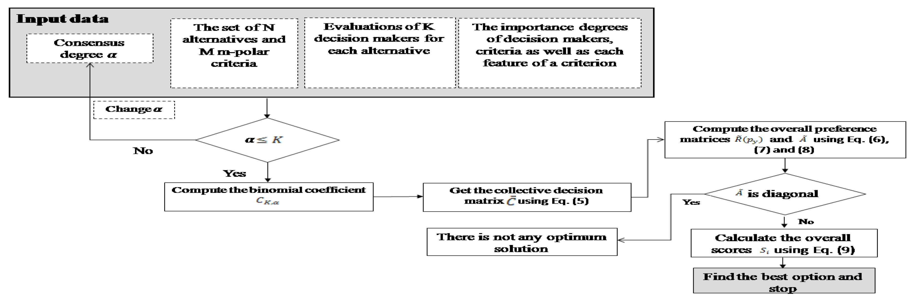
In the following, we apply the M-pFSMWM operator for solving MAGDM problems based on m-polar fuzzy soft information (Algorithm 1).The proposed procedure uses Equation (9) for ranking the preference order of objects. We also clarify the idea of the proposed method in Algorithm 1 by the given flowchart in Figure 1.

Algorithm 1. Finding the optimum solution in MAGDM problems based on M-pFSMWM operator for M-pFSSs.

Remark 2 (Analysing Algorithm 1).

Let K decision makers evaluate N number of alternatives based on M number of parameters where the m-polar fuzzy soft sets are applied to present their linguistic evaluations of the alternatives. According to Algorithm 1, we first utilize the M-pFSMWM operator to obtain a collective view of decision makers. The M-pFSMWM operator allows us to have not only partial agreement within a group, such as “almost all”, “most”, “more than half” etc., but also different choices for a partial agreement at the consensus degree α.

To this end, Algorithm 1 starts with finding the subsets ${\Delta }_{K,\alpha }(l)\subseteq \{1,2,\cdots ,K\}$ where $l=1,2,\cdots ,C_{K,\alpha }$. This helps us to check all possible cases of agreement between K decision makers at consensus level α. In fact, the value of α shows the number of possible iterations of Algorithm 1 ($1\le \alpha \le K$). By repeating Steps 1 and 2 for different value α until $\alpha \le K$, the aggregated value moves from the minimum value to the maximum value. This guaranties Algorithm 1 is convergent (please also see Theorems 2 and 4). Then, at Step 3, matrix $\overline{C}$ is driven. Each entry of $\overline{C}$ shows the performance of alternative $u_i$ based on parameter $p_y$ and the collective view of experts at degree α. In Step 4, the fuzzy preference relations $\tilde{R}(p_y)$ (for $p_y\in P$) give a comparison of objects based on the collective view of decision makers and each parameter $p_y$. The information of matrices $\tilde{R}(p_y)$ are then converted to the M-polar fuzzy soft preference relation $\tilde{A}={\left[{\tilde{\mathit{a}}}_{ij}\right]}_{N\times N}$, in Step 5, for providing comparison results where ${\tilde{\mathit{a}}}_{ij}=({\tilde{a}}_{ij}^1,{\tilde{a}}_{ij}^2,\cdots ,{\tilde{a}}_{ij}^M)\in {[0,1]}^M$ defined by ${\tilde{a}}_{ij}^y=0.5$ if ${\tilde{r}}_{ij}(p_y)=0.5$, ${\tilde{a}}_{ij}^y=1$ if ${\tilde{r}}_{ij}(p_y)>0.5$, otherwise ${\tilde{a}}_{ij}^y=0$. Moreover, if $\tilde{A}$ is an upper triangle matrix such that ${\tilde{\mathit{a}}}_{ij}=(0.5,0.5,\cdots ,0.5)$; ${\tilde{\mathit{a}}}_{ij}=(1,1,\cdots ,1)$ for $i<j$; and ${\tilde{\mathit{a}}}_{ij}=(0,0,\cdots ,0)$ for $i>j$, then we have the following descending chain $u_1\succ u_2\succ \cdots \succ u_N$ on U. If $\tilde{A}$ is a lower triangle matrix such that ${\tilde{\mathit{a}}}_{ij}=(0.5,0.5,\cdots ,0.5)$; ${\tilde{\mathit{a}}}_{ij}=(1,1,\cdots ,1)$ for $i>j$; and ${\tilde{\mathit{a}}}_{ij}=(0,0,\cdots ,0)$ for $i<j$, then we have the ascending chain $u_N\succ u_{N-1}\succ \cdots \succ u_1$ on U. However, if $\tilde{A}$ is a diagonal matrix, then there is no optimal option on U. In the last step of Algorithm 1, the best option is selected based on its rank in the resultant preference order. For MAGDM problems with benefit criteria, means more is better, the alternative with the highest score can be selected as the best option. However, for the problems dealing with cost criteria the counter condition should be considered.

5. The M-pFSIOWA and M-pFSIOWG Operators

To compare different m-polar fuzzy soft weighted aggregation operators with the proposed operator in Section 3.2, in this section, we develop the m-polar fuzzy soft induced ordered weighted average (M-pFSIOWA) operator and m-polar fuzzy soft induced ordered weighted geometric (M-pFSIOWG) operator, which are the extensions of IOWA and IOWG operators, respectively. The re-ordering step of M-pFSIOWA and M-pFSIOWG operators are defined based on the weights of arguments $\mathit{\omega }={({\omega }_1,\cdots {\omega }_K)}^T$. Since the M-pFSIOWA and M-pFSIOWG operators are defined in the domain of M-pFSSs, these new families of IOWA and IOWG operators give more general methods for aggregating data than traditional IOWA and IOWG operators.

Motivated by development of OWA operator and OWG operator for FSs [38,39] and IFSSs [21], the extensions of these two aggregation operators for M-pFSSs are defined as below.

Definition 9.

1. 

The M-pFSIOWA operator of dimension k is the mapping $M-pFSIOWA:{\bigcup }_{K\in \mathbb{N}}{(mfs(U))}^K\to mfs(U)$ such that for an associated weighting vector $\mathit{w}={(w_1,w_2,\cdots ,w_K)}^T$, where $w_j\in [0,1]$ and ${\sum }_{j=1}^K{w}_j=1$, is defined as below:

$$\begin{array}{c}\hfill M-pFSIOWA〈f_1,\cdots ,f_K〉(p_y)(u_i)=〈\sum _{j=1}^K{w}_j·F_{jyi}^1,\cdots ,\sum _{j=1}^K{w}_j·F_{jyi}^m〉\end{array}$$

(10)

2. 

The M-pFSIOWG operator of dimension k is the mapping $M-pFSIOWG:{\bigcup }_{K\in \mathbb{N}}{(mfs(U))}^K\to mfs(U)$ such that for an associated weighting vector $\mathit{w}={(w_1,w_2,\cdots ,w_K)}^T$, where $w_j\in [0,1]$ and ${\sum }_{j=1}^K{w}_j=1$, can be defined by

$$\begin{array}{c}\hfill M-pFSIOWG〈f_1,\cdots ,f_K〉(p_y)(u_i)=〈\prod _{j=1}^K{(F_{jyi}^1)}^{w_j},\cdots ,\prod _{j=1}^K{(F_{jyi}^m)}^{w_j}〉\end{array}$$

(11)

where $F_{jyi}^s$ is the kth value $f_k^s(p_y)(u_i)$ having the jth largest ${\omega }_j$ of the weighting vector $\omega ={({\omega }_1,{\omega }_2,\cdots ,{\omega }_K)}^T$ for M-pFSSs $(f_1,P),\cdots ,(f_K,P)$.

The main steps of these operations are the re-ordering step according to the weighting vector $\mathit{\omega }={({\omega }_1,{\omega }_2,\cdots ,{\omega }_K)}^T$ and then determining the associated weighting vector $\mathit{w}={(w_1,w_2,\cdots ,w_K)}^T$ to the aggregation operators M-pFSIOWA and M-pFSIOWG. Here, for each $1\le s\le m$, $1\le y\le M$, and $1\le i\le N$, the collection: $f_1^s(p_y)(u_i),\cdots ,f_K^s(p_y)(u_i)$ is re-ordered as $\langle max\left\{{\omega }_k\right\},F_{1yi}^s\rangle \ge \cdots \ge \langle min\left\{{\omega }_k\right\},F_{Kyi}^s\rangle$ where the weighting vector $\omega ={({\omega }_1,{\omega }_2,\cdots ,{\omega }_K)}^T$ shows the weights of different decision makers.

Theorem 5.

Let $(f_1,P),\cdots ,(f_K,P)$, where $K\ge 2$, is some m-polar fuzzy soft set over U and P such that for all $1\le k\le K$: $f_k(p_y)(u_i)=(f_k^1(p_y)(u_i),\cdots ,f_k^m(p_y)(u_i))\in {[0,1]}^m$ for $p_y\in P$ and $u_i\in U$, with non-negative weights ${\omega }_1,\cdots ,{\omega }_K\in [0,1]$ where ${\sum }_{k=1}^K{\omega }_k=1$. Then, the aggregated value $M-pFSIOWA〈(f_1,P),\cdots ,(f_K,P)〉$ and $M-pFSIOWG〈(f_1,P),\cdots ,(f_K,P)〉$ are still an m-polar fuzzy soft set over U.

Proof. 

Define the function $F:P\to m(U)$ such that for any $p_y\in P$ and $u_i\in U$, $F(p_y)(u_i)=M-pFSIOWA\langle f_1,\cdots ,f_K\rangle (p_y)(u_i)$ or $F(p_y)(u_i)=M-pFSIOWG\langle f_1,\cdots ,f_K\rangle (p_y)(u_i)$. Then, the assertion is trivial from $f_k^s(p_y)(u_i)\in [0,1]$, $w_k\in [0,1]$, ${\sum }_{k=1}^K{w}_k=1$, and convexity of $[0,1]$.  □

The following properties are inherited to M-pFSIOWA and M-pFSIOWG operators from IOWA operator and IOWG operator, respectively.

Theorem 6.

Let $(f_1,P),\cdots ,(f_K,P)$ be some m-polar fuzzy soft sets over U and P with non-negative weights ${\omega }_1,\cdots ,{\omega }_K\in [0,1]$ where ${\sum }_{k=1}^K{\omega }_k=1$. Let $\mathit{w}={(w_1,\cdots ,w_K)}^T$ be the associated weighting vector to the M-pFSIOWA and M-pFSIOWG operators. Then,

1. 

(Idempotency) If $(f_k,P)=(f,P)$ $\forall k$, then

$$M-pFSIOWA\langle (f_1,P),\cdots ,(f_K,P)\rangle =(f,P)$$

and

$$M-pFSIOWG\langle (f_1,P),\cdots ,(f_K,P)\rangle =(f,P)$$

2. 

(Monotonicity) If $(f_k,P)\tilde{\le }(g_k,P)$ $\forall k$, then

$$M-pFSIOWA\langle (f_1,P),\cdots ,(f_K,P)\rangle \tilde{\le }M-pFSIOWA\langle (g_1,P),\cdots ,(g_K,P)\rangle$$

and

$$M-pFSIOWG\langle (f_1,P),\cdots ,(f_K,P)\rangle \tilde{\le }M-pFSIOWG\langle (g_1,P),\cdots ,(g_K,P)\rangle$$

3. 

(Boundedness)

$$\underset{k}{min}\left\{(f_k,P)\right\}\tilde{\le }M-pFSIOWA\langle (f_1,P),\cdots ,(f_K,P)\rangle \tilde{\le }\underset{k}{max}\left\{(f_k,P)\right\}$$

and

$$\underset{k}{min}\left\{(f_k,P)\right\}\tilde{\le }M-pFSIOWG\langle (f_1,P),\cdots ,(f_K,P)\rangle \tilde{\le }\underset{k}{max}\left\{(f_k,P)\right\}$$

4. 

(Commutativity or Symmetry)

$$M-pFSIOWA\langle (f_1,P),\cdots ,(f_K,P)\rangle =M-pFSIOWA\langle (f_{\sigma (1)},P),\cdots ,(f_{\sigma (K)},P)\rangle$$

and

$$M-pFSIOWG\langle (f_1,P),\cdots ,(f_K,P)\rangle =M-pFSIOWG\langle (f_{\sigma (1)},P),\cdots ,(f_{\sigma (K)},P)\rangle$$

where σ is any permutation of $\{1,2,\cdots ,k\}$.

We can also obtain some spacial cases of M-pFSIOWA and M-pFSIOWG operators by using different choices for $\mathit{w}$.

Theorem 7.

Let $(f_1,P),\cdots ,(f_K,P)$ be some m-polar fuzzy soft sets over U and P with non-negative weights ${\omega }_1,\cdots ,{\omega }_K\in [0,1]$ where ${\sum }_{k=1}^K{\omega }_k=1$. Let $\mathit{w}={(w_1,\cdots ,w_K)}^T$ be the associated weighting vector to the M-pFSIOWA and M-pFSIOWG operators. Then, the M-pFSIOWA operator and M-pFSIOWG operator degenerate to some special aggregation operators as follows.

1. 

If $\mathit{w}={(\frac{1}{K},\cdots ,\frac{1}{K})}^T$, then

$$M-pFSIOWA\langle f_1,\cdots ,f_K\rangle (p_y)(u_i)=\langle \frac{1}{K}\sum _{j=1}^K{F}_{jyi}^1,\cdots ,\frac{1}{K}\sum _{j=1}^K{F}_{jyi}^m\rangle$$

which we call the m-polar fuzzy soft arithmetic average operator, and

$$M-pFSIOWG\langle f_1,\cdots ,f_K\rangle (p_y)(u_i)=\langle \prod _{j=1}^K{(F_{jyi}^1)}^{\frac{1}{K}},\cdots ,\prod _{j=1}^K{(F_{jyi}^m)}^{\frac{1}{K}}\rangle$$

which we call the m-polar fuzzy soft geometric average operator.

2. 

If $\mathit{w}={(1,0,\cdots ,0)}^T$, then

$$M-pFSIOWA\langle f_1,\cdots ,f_K\rangle (p_y)(u_i)=\langle \underset{j}{max}{\left\{F_{jyi}^1\right\}}_{j=1}^K,\cdots ,\underset{j}{max}{\left\{F_{jyi}^m\right\}}_{j=1}^K\rangle$$

and

$$M-pFSIOWG\langle f_1,\cdots ,f_K\rangle (p_y)(u_i)=\langle \underset{j}{max}{\left\{F_{jyi}^1\right\}}_{j=1}^K,\cdots ,\underset{j}{max}{\left\{F_{jyi}^m\right\}}_{j=1}^K\rangle$$

3. 

If $\mathit{w}={(0,\cdots ,0,1)}^T$, then

$$M-pFSIOWA\langle f_1,\cdots ,f_K\rangle (p_y)(u_i)=\langle \underset{j}{min}{\left\{F_{jyi}^1\right\}}_{j=1}^K,\cdots ,\underset{j}{min}{\left\{F_{jyi}^m\right\}}_{j=1}^K\rangle$$

and

$$M-pFSIOWG\langle f_1,\cdots ,f_K\rangle (p_y)(u_i)=\langle \underset{j}{min}{\left\{F_{jyi}^1\right\}}_{j=1}^K,\cdots ,\underset{j}{min}{\left\{F_{jyi}^m\right\}}_{j=1}^K\rangle$$

Application of M-pFSIOWA and M-pFSIOWG Operators in Group Decision-Making

In this section, similar to Algorithm 1, we apply the M-pFSIOWA operator and M-pFSIOWG operator to propose a procedure for solving MAGDM problems with M-pFS inputs as the following Algorithm 2.

Algorithm 2. Finding the optimum solution in MAGDM problems based on M-pFSIOWA or M-pFSIOWG operators for M-pFSSs.

Remark 3.

Note that Algorithm 2 starts with computing matrix $\overline{C}$ based on M-pFSIOWA or M-pFSIOWG operators rather than the M-pFSMWM operator used in Algorithm 1. In Steps 2 and 3, the entries of the resultant matrix $\overline{C}$ are used to compute the matrices $\tilde{R}(p_y)$ and $\tilde{A}$. Then, Algorithm 2 is followed similarly with Algorithm 1.

Here, by repeating Step 1 for different iteration value α until $\alpha \le K$, the aggregated value computed by M-pFSIOWA operator or M-pFSIOWG operator moves between the minimum value and the maximum value (please see Theorems 6 and 7). This guarantees Algorithm 2 is also convergent.

6. Illustrative Example

The general method for solving the MAGDM problems involves two main phases: (i) aggregation or consensus stage; and (ii) selection stage. The proposed methods in Equations (5), (10), and (11) can help us to aggregate different decision makers’ judgments about the alternatives to obtain a collective decision matrix $\overline{C}$. Further, Equations (8) and (9) provide an overall preference matrix $\tilde{A}$ and the overall score values $S_i$ for the alternatives, respectively, to cover the selection phase. In the following, we compare the proposed procedures in Algorithms 1 and 2 for MAGDM problems with m-polar fuzzy soft information by some numerical examples.

Hotel Booking Problem

In any trip, the problem of accommodation is one of the most important issues. The best option is always selected after comparing different residences based on some parameters, such as facilities and location of hotels and the budget. In this section, we discuss the problem of hotel booking, which is about selecting the best hotel to stay regarding a list of criteria, to provide a real-life example which shows the application of our method in decision-making problems. The input data are obtained from the “www.agoda.com” website, an online hotel booking service. This website provides some online questioners that passengers (guests) can fill them up to share their experiences about the hotel that they have staid. Guests are classified into the five main groups: families with young children, families with elder children, couples, solo travelers, and group of friends. Each hotel is characterized based on several criteria including “Comfort”, “Services”, “Location”, and “Food” according to the guests’ idea by numbers between zero and ten. Note that, here, all collected data are divided to ten to be in the unit interval [0, 1].

Example 2.

Let us to suppose that a travel agency in Iran wants to offer a luxury group tour for Kuala Lumpur, Malaysia, to their customers. The list of ten four-star hotels in Kuala Lumpur $H=\{h_1,\cdots ,h_{10}\}$, which are compared with each other based on the following four parameters $P=\{p_1$ = Comfort, $p_2$ = Services, $p_3$ = Location, $p_4$ = Food}, is chosen by this agency from the “www.agoda.com” website. The comments of five passengers, who filled on-line questionnaires, for five different categories “Families with Young Children”, “Families with Elder Children”, “Couples”, “Solo Travelers”, and “Group of Friends”, whose weighting vector is $\omega ={(0.25,0.25,0.2,0.15,0.15)}^T$, are selected by the travel agency as an input data of five experts. A hotel may be selected as the best accommodation place if at least three individuals of five people are satisfied with it. Since, in general, the importance degree of all criteria for different decision makers are not the same, this company defined the weighting vector $\lambda ={(0.3,0.2,0.35,0.15)}^T$ for the parameters based on the frequency of these parameters in the comments of the passengers. Let this travel agency also consider two different aspects for each parameters as follows: The parameter “Comfort” includes “Cleanliness” and “Staff Performance” with the weighting vector ${\lambda }_{{\mathit{p}}_{\mathbf{1}}}={(0.7,0.3)}^T$. The parameter “Services” includes “Facilities” and “Free Wi-Fi connectivity” with the weighting vector ${\lambda }_{{\mathit{p}}_{\mathbf{2}}}={(0.8,0.2)}^T$. The parameter “Location” includes “Close to Tourist Attractions” and “In the Green Surroundings” with the weighting vector ${\lambda }_{{\mathit{p}}_{\mathbf{3}}}={(0.7,0.3)}^T$. The parameter “Food” includes “Breakfast” and “Lunch and Dinner” with the weighting vector ${\lambda }_{{\mathit{p}}_{\mathbf{4}}}={(0.5,0.5)}^T$.

Table 3. Tabular representation of $MFSS$ $(f_1,P)$.

H	${\mathit{p}}_1$	${\mathit{p}}_2$	${\mathit{p}}_3$	${\mathit{p}}_4$
$h_1$	(0.87,0.86)	(0.7,0.86)	(0.86,0.67)	(0.58,0.81)
$h_2$	(0.7,0.7)	(0.55,0.7)	(0.74,0.73)	(0.71,0.7)
$h_3$	(0.82,0.86)	(0.6,0.86)	(0.79,0.58)	(0.6,0.8)
$h_4$	(0.83,0.81)	(0.88,0.81)	(0.84,0.78)	(0.55,0.81)
$h_5$	(0.89,0.81)	(0.64,0.81)	(0.82,0.71)	(0.69,0.84)
$h_6$	(0.68,0.69)	(0.66,0.69)	(0.82,0.77)	(0.67,0.74)
$h_7$	(0.82,0.78)	(0.73,0.78)	(0.77,0.83)	(0.66,0.8)
$h_8$	(0.78,0.8)	(0.73,0.8)	(0.74,0.8)	(0.68,0.79)
$h_9$	(0.82,0.71)	(0.8,0.71)	(0.69,0.84)	(0.64,0.76)
$h_{10}$	(0.88,0.89)	(0.86,0.89)	(0.7,0.8)	(0.83,0.85)

,

Table 4. Tabular representation of $MFSS$ $(f_2,P)$.

H	${\mathit{p}}_1$	${\mathit{p}}_2$	${\mathit{p}}_3$	${\mathit{p}}_4$
$h_1$	(0.89,0.79)	(0.72,0.84)	(0.84,0.7)	(0.59,0.8)
$h_2$	(0.74,0.76)	(0.6,0.76)	(0.77,0.75)	(0.69,0.71)
$h_3$	(0.77,0.68)	(0.73,0.77)	(0.71,0.6)	(0.57,0.69)
$h_4$	(0.78,0.72)	(0.87,0.79)	(0.85,0.65)	(0.54,0.78)
$h_5$	(0.91,0.83)	(0.8,0.91)	(0.81,0.71)	(0.66,0.88)
$h_6$	(0.69,0.7)	(0.68,0.71)	(0.82,0.75)	(0.69,0.75)
$h_7$	(0.86,0.78)	(0.8,0.86)	(0.74,0.8)	(0.66,0.8)
$h_8$	(0.78,0.78)	(0.75,0.8)	(0.74,0.77)	(0.64,0.8)
$h_9$	(0.71,0.75)	(0.85,0.69)	(0.8,0.84)	(0.49,0.72)
$h_{10}$	(0.89,0.94)	(0.86,0.89)	(0.82,0.86)	(0.85,0.92)

,

Table 5. Tabular representation of $MFSS$ $(f_3,P)$.

H	${\mathit{p}}_1$	${\mathit{p}}_2$	${\mathit{p}}_3$	${\mathit{p}}_4$
$h_1$	(0.85,0.79)	(0.74,0.85)	(0.84,0.8)	(0.64,0.81)
$h_2$	(0.71,0.69)	(0.7,0.71)	(0.74,0.66)	(0.66,0.69)
$h_3$	(0.77,0.78)	(0.73,0.8)	(0.73,0.6)	(0.57,0.73)
$h_4$	(0.83,0.76)	(0.73,0.84)	(0.82,0.7)	(0.61,0.8)
$h_5$	(0.83,0.75)	(0.69,0.82)	(0.7,0.69)	(0.65,0.79)
$h_6$	(0.69,0.7)	(0.65,0.7)	(0.8,0.76)	(0.69,0.73)
$h_7$	(0.81,0.74)	(0.8,0.82)	(0.75,0.59)	(0.65,0.78)
$h_8$	(0.76,0.73)	(0.8,0.76)	(0.71,0.6)	(0.67,0.75)
$h_9$	(0.78,0.67)	(0.75,0.8)	(0.77,0.56)	(0.57,0.73)
$h_{10}$	(0.88,0.88)	(0.8,0.86)	(0.68,0.77)	(0.77,0.84)

,

Table 6. Tabular representation of $MFSS$ $(f_4,P)$.

H	${\mathit{p}}_1$	${\mathit{p}}_2$	${\mathit{p}}_3$	${\mathit{p}}_4$
$h_1$	(0.83,0.82)	(0.6,0.83)	(0.75,0.7)	(0.68,0.83)
$h_2$	(0.72,0.72)	(0.4,0.71)	(0.69,0.71)	(0.64,0.7)
$h_3$	(0.74,0.76)	(0.8,0.76)	(0.75,0.59)	(0.62,0.68)
$h_4$	(0.88,0.84)	(0.74,0.89)	(0.83,0.77)	(0.69,0.84)
$h_5$	(0.79,0.79)	(0.64,0.83)	(0.75,0.76)	(0.61,0.82)
$h_6$	(0.69,0.69)	(0.76,0.68)	(0.79,0.81)	(0.66,0.72)
$h_7$	(0.81,0.76)	(0.53,0.81)	(0.73,0.84)	(0.66,0.78)
$h_8$	(0.73,0.72)	(0.7,0.73)	(0.68,0.79)	(0.64,0.72)
$h_9$	(0.82,0.81)	(0.6,0.89)	(0.79,0.87)	(0.71,0.79)
$h_{10}$	(0.87,0.87)	(1,0.87)	(0.7,0.76)	(0.75,0.83)

and

Table 7. Tabular representation of $MFSS$ $(f_5,P)$.

H	${\mathit{p}}_1$	${\mathit{p}}_2$	${\mathit{p}}_3$	${\mathit{p}}_4$
$h_1$	(0.87,0.6)	(0.84,0.87)	(0.93,0.84)	(0.6,0.9)
$h_2$	(0.74,0.8)	(0.74,0.74)	(0.8,0.74)	(0.64,0.74)
$h_3$	(0.85,0.8)	(0.8,0.8)	(0.81,0.8)	(0.62,0.8)
$h_4$	(0.81,0.84)	(0.77,0.76)	(0.77,0.76)	(0.59,0.77)
$h_5$	(0.8,0.8)	(0.76,0.77)	(0.84,0.77)	(0.61,0.76)
$h_6$	(0.67,0.8)	(0.72,0.78)	(0.67,0.78)	(0.66,0.72)
$h_7$	(0.78,0.69)	(0.76,0.74)	(0.78,0.74)	(0.64,0.76)
$h_8$	(0.77,0.72)	(0.76,0.72)	(0.79,0.72)	(0.67,0.76)
$h_9$	(0.65,0.6)	(0.69,0.76)	(0.78,0.76)	(0.44,0.69)
$h_{10}$	(0.88,0.86)	(0.82,0.66)	(0.88,0.66)	(0.77,0.82)

show the evaluation of the hotels based on these five passengers’ comments by using m-polar fuzzy soft sets.

Since the required consensus degree is $\alpha =3$, then $L=\frac{5!}{3!(5-3)!}=10$. All 10 different combinations of three of five objects can be listed as follows: ${\Delta }_{5,3}(1)=\{1,2,3\}$, ${\Delta }_{5,3}(2)=\{1,2,4\}$, ${\Delta }_{5,3}(3)=\{1,2,5\}$, ${\Delta }_{5,3}(4)=\{1,3,4\}$, ${\Delta }_{5,3}(5)=\{1,3,5\}$, ${\Delta }_{5,3}(6)=\{1,4,5\}$, ${\Delta }_{5,3}(7)=\{2,3,4\}$, ${\Delta }_{5,3}(8)=\{2,3,5\}$, ${\Delta }_{5,3}(9)=\{2,4,5\}$, and ${\Delta }_{5,3}(10)=\{3,4,5\}$. (Steps 1,2).

Step 3. Utilize data given in Table 3, Table 4, Table 5, Table 6 and Table 7 with the weighting vector $\omega ={(0.25,0.25,0.2,0.15,0.15)}^T$ and M-pFSMWM operator proposed in Theorem 3 to get the collective matrix $\overline{C}={\left[{\overline{\mathit{c}}}_{iy}\right]}_{10\times 4}$ as below:

$$\begin{array}{c}\hfill \overline{C}=\left[\begin{array}{cccc}(0.597,0.553)& (0.49,0.588)& (0.588,0.469)& (0.406,0.56)\\ (0.49,0.484)& (0.385,0.49)& (0.518,0.4745)& (0.465,0.484)\\ (0.539,0.476)& (0.438,0.539)& (0.497,0.406)& (0.399,0.483)\\ (0.546,0.504)& (0.525,0.553)& (0.576,0.455)& (0.378,0.546)\\ (0.587,0.531)& (0.448,0.567)& (0.537,0.485)& (0.456,0.558)\\ (0.476,0.483)& (0.456,0.483)& (0.562,0.525)& (0.469,0.512)\\ (0.568,0.522)& (0.511,0.546)& (0.518,0.52)& (0.456,0.548)\\ (0.534,0.516)& (0.511,0.536)& (0.5,0.5005)& (0.448,0.529)\\ (0.497,0.473)& (0.53,0.483)& (0.483,0.546)& (0.3455,0.504)\\ (0.616,0.617)& (0.566,0.605)& (0.478,0.542)& (0.545,0.589)\end{array}\right]\end{array}$$

Step 4. Utilize Equation (6) to compute matrices $\tilde{R}(p_y)={\left[{\tilde{r}}_{ij}(p_y)\right]}_{10\times 10}$, where $y=1,2,3,4$, as follows:

$$\begin{array}{c}\hfill \tilde{R}(p_1)=\left[\begin{array}{cccccccccc}0.5& 0.54& 0.53& 0.52& 0.506& 0.55& 0.51& 0.52& 0.54& 0.49\\ 0.45& 0.5& 0.48& 0.48& 0.46& 0.505& 0.47& 0.48& 0.49& 0.44\\ 0.47& 0.51& 0.5& 0.49& 0.47& 0.52& 0.48& 0.49& 0.51& 0.45\\ 0.47& 0.52& 0.506& 0.5& 0.48& 0.52& 0.49& 0.502& 0.52& 0.46\\ 0.49& 0.53& 0.52& 0.51& 0.5& 0.54& 0.507& 0.51& 0.53& 0.48\\ 0.45& 0.49& 0.47& 0.47& 0.45& 0.5& 0.46& 0.47& 0.49& 0.43\\ 0.48& 0.53& 0.51& 0.509& 0.49& 0.53& 0.5& 0.51& 0.53& 0.47\\ 0.47& 0.51& 0.504& 0.49& 0.48& 0.52& 0.48& 0.5& 0.51& 0.46\\ 0.45& 0.5008& 0.48& 0.47& 0.46& 0.506& 0.46& 0.48& 0.5& 0.44\\ 0.51& 0.55& 0.54& 0.53& 0.51& 0.56& 0.52& 0.53& 0.55& 0.5\end{array}\right]\end{array}$$

$$\begin{array}{c}\hfill \tilde{R}(p_2)=\left[\begin{array}{cccccccccc}0.5& 0.55& 0.52& 0.48& 0.51& 0.52& 0.49& 0.49& 0.49& 0.47\\ 0.44& 0.5& 0.46& 0.43& 0.46& 0.46& 0.43& 0.44& 0.43& 0.41\\ 0.47& 0.53& 0.5& 0.46& 0.49& 0.49& 0.46& 0.47& 0.46& 0.44\\ 0.51& 0.56& 0.53& 0.5& 0.52& 0.53& 0.506& 0.506& 0.504& 0.48\\ 0.48& 0.53& 0.507& 0.47& 0.5& 0.505& 0.47& 0.47& 0.47& 0.45\\ 0.47& 0.53& 0.501& 0.46& 0.49& 0.5& 0.47& 0.47& 0.46& 0.44\\ 0.504& 0.56& 0.53& 0.49& 0.52& 0.52& 0.5& 0.501& 0.49& 0.47\\ 0.503& 0.56& 0.52& 0.49& 0.52& 0.52& 0.49& 0.5& 0.49& 0.47\\ 0.505& 0.56& 0.53& 0.49& 0.52& 0.53& 0.501& 0.502& 0.5& 0.47\\ 0.53& 0.58& 0.55& 0.51& 0.54& 0.55& 0.52& 0.52& 0.52& 0.5\end{array}\right]\end{array}$$

$$\begin{array}{c}\hfill \tilde{R}(p_3)=\left[\begin{array}{cccccccccc}0.5& 0.52& 0.54& 0.505& 0.51& 0.5006& 0.51& 0.52& 0.52& 0.52\\ 0.47& 0.5& 0.51& 0.48& 0.49& 0.47& 0.49& 0.502& 0.501& 0.503\\ 0.45& 0.48& 0.5& 0.46& 0.47& 0.46& 0.47& 0.48& 0.48& 0.48\\ 0.49& 0.51& 0.53& 0.5& 0.508& 0.49& 0.509& 0.51& 0.51& 0.52\\ 0.48& 0.508& 0.52& 0.49& 0.5& 0.48& 0.501& 0.51& 0.509& 0.51\\ 0.49& 0.52& 0.53& 0.505& 0.51& 0.5& 0.51& 0.52& 0.52& 0.52\\ 0.48& 0.506& 0.52& 0.49& 0.49& 0.48& 0.5& 0.509& 0.508& 0.51\\ 0.47& 0.49& 0.51& 0.48& 0.48& 0.47& 0.49& 0.5& 0.49& 0.501\\ 0.47& 0.49& 0.51& 0.48& 0.49& 0.47& 0.49& 0.5008& 0.5& 0.502\\ 0.47& 0.49& 0.51& 0.47& 0.48& 0.47& 0.48& 0.49& 0.49& 0.5\end{array}\right]\end{array}$$

$$\begin{array}{c}\hfill \tilde{R}(p_4)=\left[\begin{array}{cccccccccc}0.5& 0.504& 0.52& 0.51& 0.48& 0.49& 0.49& 0.49& 0.53& 0.46\\ 0.49& 0.5& 0.51& 0.506& 0.48& 0.49& 0.48& 0.49& 0.52& 0.45\\ 0.47& 0.48& 0.5& 0.48& 0.46& 0.47& 0.46& 0.47& 0.509& 0.43\\ 0.48& 0.49& 0.51& 0.5& 0.47& 0.48& 0.47& 0.48& 0.52& 0.44\\ 0.51& 0.51& 0.53& 0.52& 0.5& 0.508& 0.502& 0.509& 0.54& 0.47\\ 0.503& 0.508& 0.52& 0.51& 0.49& 0.5& 0.49& 0.501& 0.53& 0.46\\ 0.509& 0.51& 0.53& 0.52& 0.49& 0.505& 0.5& 0.506& 0.54& 0.46\\ 0.502& 0.507& 0.52& 0.51& 0.49& 0.49& 0.49& 0.5& 0.53& 0.46\\ 0.46& 0.47& 0.49& 0.47& 0.45& 0.46& 0.45& 0.46& 0.5& 0.42\\ 0.54& 0.54& 0.56& 0.55& 0.52& 0.53& 0.53& 0.53& 0.57& 0.5\end{array}\right]\end{array}$$

Step 5. Now, the matrix $\tilde{A}={\left[{\tilde{\mathit{a}}}_{ij}\right]}_{10\times 10}$ is computed, using information given in matrices $\tilde{R}(p_y)$ ($y=1,2,3,4$), to obtain a collective four-polar fuzzy soft preference matrix as the following:

Step 6. Calculate the score value of each alternatives according to the collective 4-polar fuzzy soft preference matrix $\tilde{A}$ and Equation (9) as the following: $S_1=6.95$, $S_2=2.15$, $S_3=1.25$, $S_4=5.85$, $S_5=6$, $S_6=4.1$, $S_7=5.8$, $S_8=3.65$, $S_9=3.05$, and $S_{10}=6.2$.

Step 7. Thus, we have: $h_1\succ h_{10}\succ h_5\succ h_4\succ h_7\succ h_6\succ h_8\succ h_9\succ h_2\succ h_3$. Thus, the first hotel, called $h_1$, is the best option to stay while $h_3$ should not be selected for accommodation.

In Example 2, the desirable alternative is accepted by most of the decision makers where “most” is interpreted as acceptable by $60\%$ of decision makers, i.e., at least three individuals of total five decision makers are satisfied. To check the impact of consensus degree on the final solution, we compare the obtained results in Example 2 with the result of full agreement, given by the following example in which $\alpha =5$ is used as the consensus degree.

Example 3.

(Example 2 continued) Let us reconsider the “Hotel Booking Problem” involving M-pFSSs $(f_1,P),(f_2,P),(f_3,P),(f_4,P),$ and $(f_5,P)$ which is discussed earlier in Example 2 where $H=\{h_1,\cdots ,h_{10}\}$ is the set of alternatives and $P=\{p_1,p_2,p_3,p_4\}$ is the set of parameters.

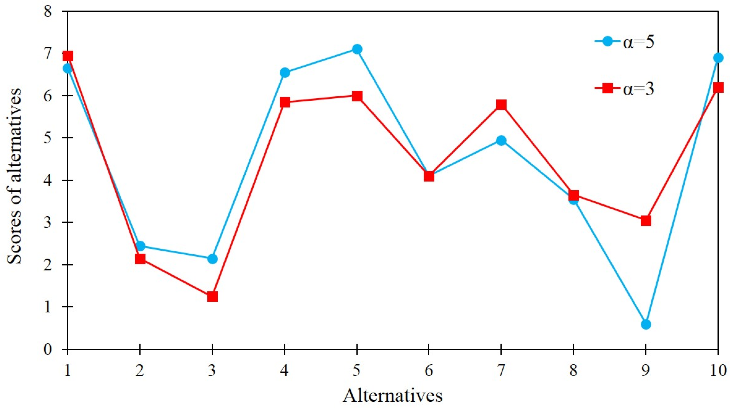
Here, the proposed Algorithm 1 is applied for case $\alpha =5$, where $L=C_{5,5}=1$ and ${\Delta }_{5,5}(1)=\{1,2,3,4,5\}$, to get the most desirable alternative based on a unanimous consensus. After applying Algorithm 1, the scores of alternatives are computed as follows: $S_1=6.65$, $S_2=2.45$, $S_3=2.15$, $S_4=6.55$, $S_5=7.1$, $S_6=4.1$, $S_7=4.95$, $S_8=3.55$, $S_9=0.6$, and $S_{10}=6.9$. Therefore, we get: $h_5\succ h_{10}\succ h_1\succ h_4\succ h_7\succ h_6\succ h_8\succ h_2\succ h_3\succ h_9$ which shows $h_5$ is the alternative accepted by all decision makers. Hotel $h_1$, which is the best option for accommodation according to the most decision makers’ views, is the third most desirable alternative. Figure 2 shows the effect of different consensus degrees $\alpha =3$ and $\alpha =5$ on scores of alternatives.

Now, we reconsider Examples 2 and 3 according to Algorithm 2 which is based on M-pFSIOWA operator and M-pFSIOWG operator.

Example 4.

(Examples 2 and 3 continued) To apply Algorithm 2 for solving MAGDM problem given in Examples 2 and 3, we first need to re-order the M-pFSSs $(f_1,P),\cdots ,(f_5,P)$ based on weighting vector $\omega ={(0.25,0.25,0.2,0.15,0.15)}^T$ for the decision makers $f_1,\cdots ,f_5$. Subsequently, we get: $F_{1yi}^s=f_1^s(p_y)(u_i)$, $F_{2yi}^s=f_2^s(p_y)(u_i)$, $F_{3yi}^s=f_3^s(p_y)(u_i)$, $F_{4yi}^s=f_4^s(p_y)(u_i)$, and $F_{5yi}^s=f_5^s(p_y)(u_i)$ for $s=1,2$; $i=1,2,\cdots ,10$; and $y=1,2,3,4$. The associated weighting vector $\mathit{w}=(w_1,w_2,\cdots ,w_5)$ is then generated by $w_k=Q(\frac{k}{5})-Q(\frac{k-1}{5})$ for $k=1,\cdots ,5$ where $Q(.)$ is a quantifier function $Q:[0,1]\to [0,1]$.

First, for case “most of the decision makers” (i.e., $\alpha =3$), where “most” is interpreted as $60\%$ or $\frac{3}{5}$ of all data, the quantifier function may be defined by

$$\begin{array}{c}\hfill Q_{most}(z)=\left\{\begin{array}{cc}0\hfill & if z\le \frac{1}{5}\hfill \\ \frac{z-\raisebox{1ex}{$1$}\!\left/ \!\raisebox{-1ex}{$5$}\right.}{\raisebox{1ex}{$2$}\!\left/ \!\raisebox{-1ex}{$5$}\right.}\hfill & if \frac{1}{5}<z<\frac{3}{5}\hfill \\ 1\hfill & if z\ge \frac{3}{5}\hfill \end{array}\right.\end{array}$$

(12)

Therefore, we get $w_1=w_4=w_5=0$, $w_2=w_3=0.5$ and subsequently $\mathit{w}={(0,0.5,0.5,0,0)}^T$. Thus, by using Equations (10) and (11), we have:

$${[M-pFSIOWA\langle f_1,f_2,f_3,f_4,f_5\rangle ]}^s(p_y)(u_i)=\frac{F_{2yi}^s+F_{3yi}^s}{2}$$

and

$${[M-pFSIOWG\langle f_1,f_2,f_3,f_4,f_5\rangle ]}^s(p_y)(u_i)=\sqrt{F_{2yi}^s·F_{3yi}^s}$$

for $s=1,2$; $i=1,2,\cdots ,10$; and $y=1,2,3,4$.

For the unanimous consensus (i.e., $\alpha =5$), the quantifier function may be defined by

$$\begin{array}{c}\hfill Q_{all}(z)=\left\{\begin{array}{cc}0\hfill & if z<1\hfill \\ 1\hfill & if z=\frac{5}{5}=1\hfill \end{array}\right.\end{array}$$

(13)

Thus, the weighting vector is $\mathit{w}={(0,0,0,0,1)}^T$. Subsequently, by using Equations (10) and (11), we have

$${[M-pFSIOWA\langle f_1,f_2,f_3,f_4,f_5\rangle ]}^s(p_y)(u_i)=F_{5yi}^s$$

and

$${[M-pFSIOWG\langle f_1,f_2,f_3,f_4,f_5\rangle ]}^s(p_y)(u_i)=F_{5yi}^s$$

for $s=1,2$; $i=1,2,\cdots ,10$; and $y=1,2,3,4$.

Thus, based on the M-pFSIOWA operator and M-pFSIOWG operator the resultant collective m-polar fuzzy soft matrix $\overline{C}={[{\overline{\overrightarrow{c}}}_{iy}]}_{10\times 4}$ where

$${\overline{\mathbf{c}}}_{iy}=\left(\frac{f_2^1(p_y)(u_i)+f_3^1(p_y)(u_i)}{2},\frac{f_2^2(p_y)(u_i)+f_3^2(p_y)(u_i)}{2}\right);$$

$${\overline{\mathbf{c}}}_{iy}=\left(\sqrt{f_2^1(p_y)(u_i)·f_3^1(p_y)(u_i)},\sqrt{f_2^2(p_y)(u_i)·f_3^2(p_y)(u_i)}\right);$$

and

$${\overline{\mathbf{c}}}_{iy}=\left(f_5^1(p_y)(u_i),f_5^2(p_y)(u_i)\right)$$

is derived for different cases $\alpha =3$ and $\alpha =5$, respectively. Then, Steps 4–7 of Algorithm 1 are used to compare the scores of alternatives for both cases $\alpha =3$ and $\alpha =5$.

The obtained results from M-pFSMWM, M-pFSIOWA, and M-pFSIOWG operators are reported in

Table 8. Comparison results of Examples 2–4 for different M-pFS-based aggregation methods.

Aggregation Methods	$\mathit{\alpha }$	Number of Computational Steps	Scores of Alternatives (${\mathit{S}}_{\mathit{i}}$)
			${\mathit{h}}_1$	${\mathit{h}}_2$	${\mathit{h}}_3$	${\mathit{h}}_4$	${\mathit{h}}_5$	${\mathit{h}}_6$	${\mathit{h}}_7$	${\mathit{h}}_8$	${\mathit{h}}_9$	${\mathit{h}}_{10}$
M-pFSMWM	$\alpha =3$	18	6.95	2.15	1.25	5.85	6	4.1	5.8	3.65	3.05	6.2
M-pFSMWM	$\alpha =5$	9	6.65	2.45	2.15	6.55	7.1	4.1	4.95	3.55	0.6	6.9
M-pFSIOWA	$\alpha =3$	9	6.6	1.8	1.45	5.65	5.825	3.825	5.15	3.375	3.375	7.95
M-pFSIOWA	$\alpha =5$	9	7.65	3.875	7	3.8	5.9	1.025	2.85	3.6	1.4	7.9
M-pFSIOWG	$\alpha =3$	9	6.75	1.8	1.45	5.65	5.85	3.9	5.15	3.3	3.2	7.95
M-pFSIOWG	$\alpha =5$	9	7.65	3.875	7	3.8	5.9	1.025	2.85	3.6	1.4	7.9

α refers to consensus degree.

.

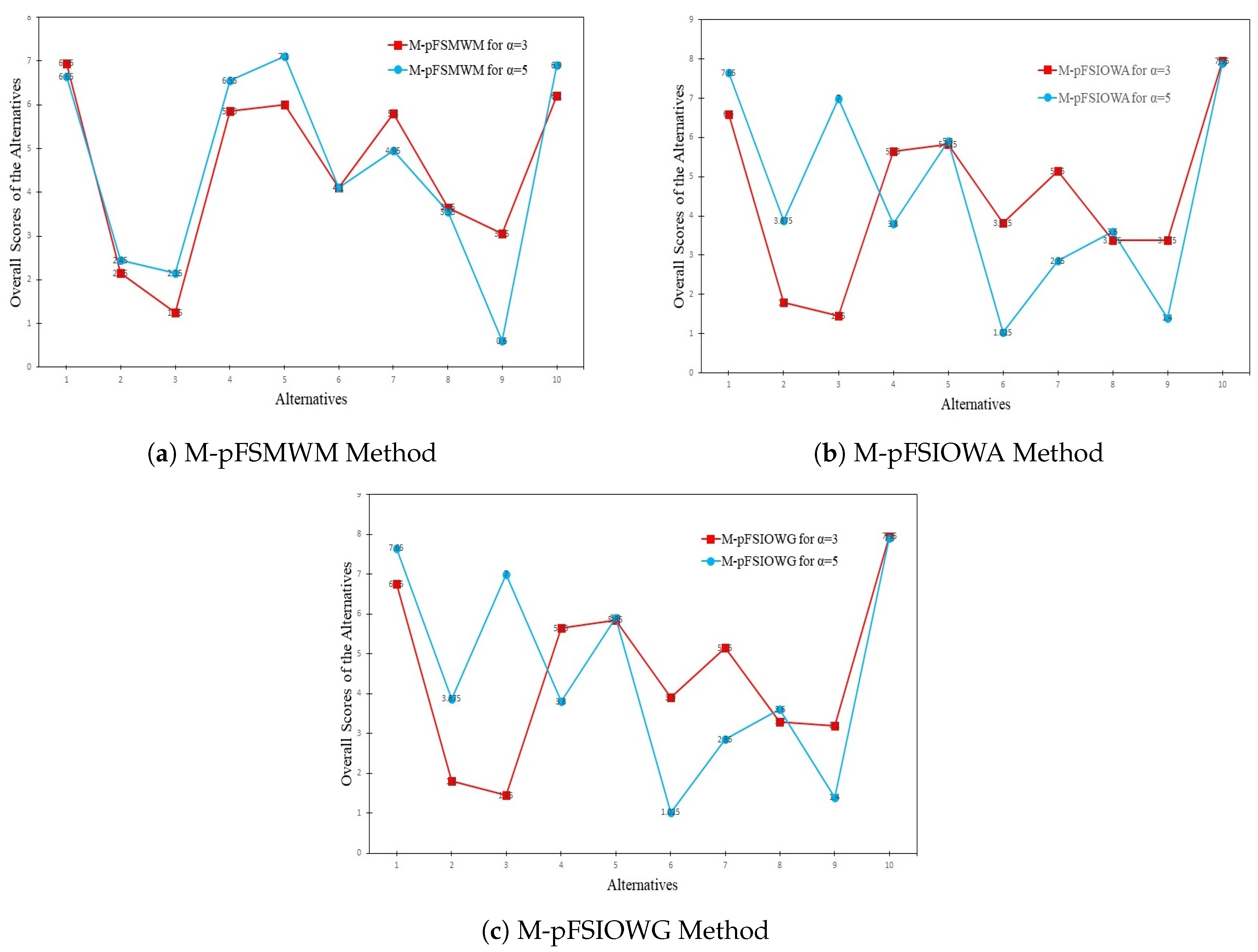
It can be seen that, for case $\alpha =5$, $h_{10}$ is the best option selected by all methods. For $\alpha =3$, the M-pFSMWM method selects $h_1$, however the tenth hotel, $h_{10}$, is chosen by the two other methods. Accordingly, the scores of alternatives for different consensus degrees $\alpha =3$ and $\alpha =5$ are compared in Figure 3a–c.

7. Discussion

To date, various soft set-based techniques have been applied to solve decision-making problems. Some of them have proposed novel methodology to find the solution [18,22,27,28], while some authors have made effort to adapt the well-known decision-making methods, such as SAW, TOPSIS, entropy, OWA, and OWG to the soft set theory [15,16,21,40,41]. However, a technique to solve decision-making problems based on m-polar fuzzy soft information has not been studied yet. Thus, new methodologies are proposed to handle the consensus stage and selection stage of MAGDM problem with M-pFS inputs.

For aggregating input data which take their values from ${[0,1]}^m$, some new m-polar aggregating methods, called M-pFSMWM operator, M-pFSIOWA operator, and M-pFSIOWG operator, are developed in Section 3 and Section 5. The properties comparison of these operators are summarized in

Table 9. Properties comparison of different aggregation operators.

Operators	Idempotency	Boundedness	Monotonicity	Symmetry	Flexible by Consensus Degree α	Flexible for Different Choices of K
M-pFSMWM	Yes	Yes	Yes	Yes	Yes	Yes
M-pFSIOWA	Yes	Yes	Yes	Yes	No	No
M-pFSIOWG	Yes	Yes	Yes	Yes	No	No

. It can be seen that the most interesting property of M-pFSMWM operator is it is sensitive for different scenarios of a partial agreement at the consensus degree α. This characteristic makes the M-pFSIOWA operator more adaptable for MAGDM problem in which not only the number of individuals satisfying an alternative is important but also the weight of decision makers who agree with this decision affect the final output. Moreover, by changing the value of consensus degree α different cases of agreement are obtained. In particular, when $\alpha \to K$, the partial agreement becomes a full agreement.

To reach the process of selection, we propose two procedures in Section 4.2, Algorithm 1 where the consensus stage is reached based on the new M-pFSMWM operator, and Section 5, Algorithm 2 in which the consensus stage is obtained by M-pFSIOWA or M-pFSIOWG operators are extended based on IOWA and IOWG, respectively. To reach the selection stage a new score value function, described by Equation (9), is applied. The main advantage of the proposed formulation is to rank and compare objects based on a collective m-polar fuzzy soft preference relationship. This allows us to have a ranking system of alternatives, from the most preferred element to the least preferred element, which may include some incomparable objects because of preference relationships nature.

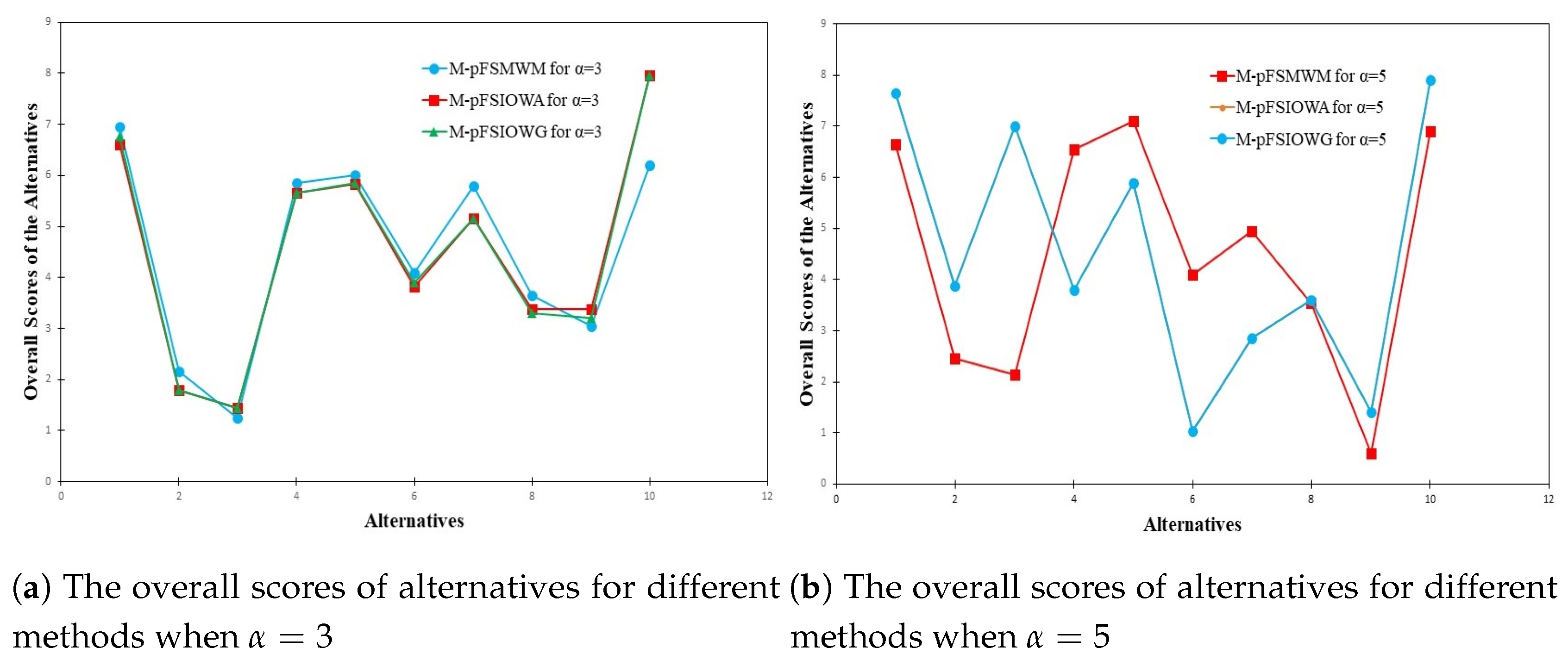
Illustrative examples, given in Examples 2 and 3, show the application of Algorithm 1 to analyze MAGDM problems with multi-polar fuzzy soft information. The obtained results are then compared with the m-polar fuzzy soft extensions of two well-known aggregation operators IOWA and IOWG, i.e., M-pFSIOWA and M-pFSIOWG, in Example 4.

Table 10. Comparison of the alternatives’ preference orders for different methods.

Methods	Consensus Degree α	Preference Order
M-pFSMWM	3	$h_1\succ h_{10}\succ h_5\succ h_4\succ h_7\succ h_6\succ h_8\succ h_9\succ h_2\succ h_3$
M-pFSMWM	5	$h_5\succ h_{10}\succ h_1\succ h_4\succ h_7\succ h_6\succ h_8\succ h_2\succ h_3\succ h_9$
M-pFSIOWA	3	$h_{10}\succ h_1\succ h_5\succ h_4\succ h_7\succ h_6\succ h_8\succ h_9\succ h_2\succ h_3$
M-pFSIOWA	5	$h_{10}\succ h_1\succ h_3\succ h_5\succ h_2\succ h_4\succ h_8\succ h_7\succ h_9\succ h_6$
M-pFSIOWG	3	$h_{10}\succ h_1\succ h_5\succ h_4\succ h_7\succ h_6\succ h_8\succ h_9\succ h_2\succ h_3$
M-pFSIOWG	5	$h_{10}\succ h_1\succ h_3\succ h_5\succ h_2\succ h_4\succ h_8\succ h_7\succ h_9\succ h_6$

makes a comparison of the preference orders of the alternatives for methods using different aggregation operators including the new proposed M-pFSMWM method, the m-polar fuzzy soft induced ordered weighted average (M-pFSIOWA) method, and the m-polar fuzzy soft induced ordered weighted geometric (M-pFSIOWG) method. As can be seen, Hotel $h_{10}$ is the best option for staying based on the all discussed methods except the M-pFSMWM-based method, where $h_{10}$ is considered as the best second option for accommodation. According to final preference order obtained based on the M-pFSMWM operator, Hotel $h_1$, which has the second place based on the other methods, is the best option accepted by the majority, i.e., $60\%$, of decision makers. Hotel $h_5$ is the best place to stay in terms of all decision makers. The analysis derived in Table 10 shows a good agreement among thees methods, however the number of computational steps in M-pFSMWM-based algorithm is $C_{K,\alpha }+1$ in comparison with $K+2$ stages in Algorithm 2. On the other hand, the main disadvantage of M-pFSIOWA and M-pFSIOWG methods is that there is no unique approach to determine the associated weighting vector $\mathit{w}$ related to the aggregation operators M-pFSIOWA and M-pFSIOWG. Finally, in Figure 4a, the overall scores of alternatives based on the different methods for case $\alpha =3$ are shown. Figure 4b shows the scores of alternatives obtained by using different methods for case $\alpha =5$. Note that, using some relative preference matrices to find the scores of alternatives in all methods, leads to record a similar trend in Figure 4b.

8. Conclusions

Traditional aggregation operators, which usually deal with uni-polar information, fail to aggregate m-polar fuzzy soft information taking their values from ${[0,1]}^m$. This study proposes a new aggregation method for processing the MAGDM problems with m-polar fuzzy soft information in which both attributes and experts have different weights. For this purpose, firstly the concept of m-polar fuzzy soft sets is introduced. Then, the new aggregation operator M-pFSMWM in the domain of m-polar fuzzy soft sets is defined. The advantage of proposed M-pFSMWM operator is to be sensitive for different partial agreement scenarios at a consensus degree α. Further, the m-polar fuzzy soft induced ordered weighted average (M-pFSIOWA) operator and the m-polar fuzzy soft induced ordered weighted geometric (M-pFSIOWG) operator, which are the extensions of IOWA and IOWG operators, respectively, are developed. Some desirable properties of M-pFSMWM, M-pFSIOWA, and M-pFSIOWG operators, such as idempotency, monotonicity, and commutativity are also studied. The characteristics of the proposed M-pFSMWM operator shows it is more adaptable for a wider range of MAGDM problems in comparison with M-pFSIOWA and M-pFSIOWG operators. In addition, a procedure for ranking m-polar fuzzy soft data based on a new score value function is proposed. Then, two algorithms are designed to MAGDM problems based on M-pFSMWM, M-pFSIOWA, and M-pFSIOWG operators. Finally, to show the efficiency of proposed methods, some numerical examples are discussed.

References

- Dubois, D.; Prade, H. Weighted minimum and maximum operations in fuzzy set theory. Inf. Sci. 1986, 39, 205–210. [Google Scholar] [CrossRef]
- Fagin, R.; Wimmers, E.L. A formula for incorporating weights into scoring rules. Theor. Comput. Sci. 2000, 239, 309–338. [Google Scholar] [CrossRef]
- Yager, R.R. A new methodology for ordinal multiobjective decisions based on fuzzy sets. In Readings in Fuzzy Sets for Intelligent Systems; Elsevier: San Francisco, CA, USA, 1993; pp. 751–756. [Google Scholar]
- Yager, R.R. On ordered weighted averaging aggregation operators in multicriteria decisionmaking. In Readings in Fuzzy Sets for Intelligent Systems; Elsevier: San Francisco, CA, USA, 1993; pp. 80–87. [Google Scholar]
- Chiclana, F.; Herrera, F.; Herrera-Viedma, E. The ordered weighted geometric operator: Properties and application in MCDM Problems. In Technologies for Constructing Intelligent Systems 2; Physica: Heidelberg, Germany, 2002; pp. 173–183. [Google Scholar]
- Yager, R.R.; Filev, D.P. Induced ordered weighted averaging operators. IEEE Trans. Syst. Man Cybern. B Cybern. 1999, 29, 141–150. [Google Scholar] [CrossRef] [PubMed]
- Xu, Z.S.; Da, Q.L. An overview of operators for aggregating information. Int. J. Intell. Inf. Technol. 2003, 18, 953–969. [Google Scholar] [CrossRef]
- Kacprzyk, J. Group decision making with a fuzzy linguistic majority. Fuzzy Sets Syst. 1986, 18, 105–118. [Google Scholar] [CrossRef]
- Kacprzyk, J.; Fedrizzi, M.; Nurmi, H. Group decision making and consensus under fuzzy preferences and fuzzy majority. Fuzzy Sets Syst. 1992, 49, 21–31. [Google Scholar] [CrossRef]
- Molodtsov, D. Soft set theory—First results. Comput. Math. Appl. 1999, 37, 19–31. [Google Scholar] [CrossRef] [Green Version]
- Zadeh, L.A. Fuzzy sets. Inf. Control 1965, 8, 338–353. [Google Scholar] [CrossRef] [Green Version]
- Maji, P.K.; Biswas, R.; Roy, A.R. Fuzzy soft sets. J. Fuzzy Math. 2001, 9, 589–602. [Google Scholar]
- Maji, P.K.; Biswas, R.; Roy, A.R. Intuitionistic fuzzy soft sets. J. Fuzzy Math. 2001, 9, 677–692. [Google Scholar]
- Maji, P.K.; Roy, A.R.; Biswas, R. An application of soft sets in a decision making problem. Comput. Math. Appl. 2002, 44, 1077–1083. [Google Scholar] [CrossRef]
- Roy, A.R.; Maji, P.K. A fuzzy soft set theoretic approach to decision making problems. J. Comput. Appl. Math. 2007, 203, 412–418. [Google Scholar] [CrossRef]
- Alcantud, J.C.R. A novel algorithm for fuzzy soft set based decision making from multiobserver input parameter data set. Inf. Fusion 2016, 29, 142–148. [Google Scholar] [CrossRef]
- Cagman, N.; Enginoglu, S.; Citak, F. Fuzzy soft set theory and its applications. Iran. J. Fuzzy Syst. 2011, 8, 137–147. [Google Scholar]
- Cagman, N.; Enginoglu, S. Fuzzy soft matrix theory and its application in decision making. Iran. J. Fuzzy Syst. 2012, 9, 109–119. [Google Scholar]
- Guan, X.; Li, Y.; Feng, F. A new order relation on fuzzy soft sets and its application. Soft Comput. 2013, 17, 63–70. [Google Scholar] [CrossRef]
- Zhang, Z. A rough set approach to intuitionistic fuzzy soft set based decision making. Appl. Math. Model. 2012, 36, 4605–4633. [Google Scholar] [CrossRef]
- Mao, J.; Yao, D.; Wang, C. Group decision making methods based on intuitionistic fuzzy soft matrices. Appl. Math. Model. 2013, 37, 6425–6436. [Google Scholar] [CrossRef]
- Das, S.; Kar, S. Group decision making in medical system: An intuitionistic fuzzy soft set approach. Appl. Soft Comput. 2014, 24, 196–211. [Google Scholar] [CrossRef]
- Zhang, Z.; Zhang, S. A novel approach to multi attribute group decision making based on trapezoidal interval type-2 fuzzy soft sets. Appl. Math. Model. 2013, 37, 4948–4971. [Google Scholar] [CrossRef]
- Pandey, A.; Kumar, A. A note on “A novel approach to multi attribute group decision making based on trapezoidal interval type-2 fuzzy soft sets”. Appl. Math. Model. 2017, 41, 691–693. [Google Scholar] [CrossRef]
- Tao, Z.; Chen, H.; Zhou, L.; Liu, J. 2-Tuple linguistic soft set and its application to group decision making. Soft Comput. 2015, 19, 1201–1213. [Google Scholar] [CrossRef]
- Zhu, K.; Zhan, J. Fuzzy parameterized fuzzy soft sets and decision making. Int. J. Mach. Learn. Cybern. 2016, 7, 1207–1212. [Google Scholar] [CrossRef]
- Zahedi-Khameneh, A.; Kılıçman, A.; Salleh, A.R. An adjustable approach to multi-criteria group decision-making based on a preference relationship under fuzzy soft information. Int. J. Fuzzy Syst. 2017, 19, 1840–1865. [Google Scholar] [CrossRef]
- Zahedi-Khameneh, A.; Kılıçman, A.; Salleh, A.R. Application of a preference relationship in decision-making based on intuitionistic fuzzy soft sets. J. Intell. Fuzzy Syst. 2018, 34, 123–139. [Google Scholar] [CrossRef]
- Mesiarova, A.; Lazaro, J. Bipolar aggregation operators. Proc. AGOP 2003, 2003, 119–123. [Google Scholar]
- Mesiarova-Zemankova, A.; Ahmad, K. Extended multi-polarity and multi-polar-valued fuzzy sets. Fuzzy Sets Syst. 2014, 234, 61–78. [Google Scholar] [CrossRef]
- Mesiarova-Zemankova, A. Multi-polar t-conorms and uninorms. Inf. Sci. 2015, 301, 227–240. [Google Scholar] [CrossRef]
- Medina, J.; Ojeda-Aciego, M. Multi-adjoint t-concept lattices. Inf. Sci. 2010, 180, 712–725. [Google Scholar] [CrossRef]
- Pozna, C.; Minculete, N.; Precup, R.E.; Koczy, L.; Ballagi, A. Signatures: Definitions, operators and applications to fuzzy modelling. Fuzzy Sets Syst. 2012, 201, 86–104. [Google Scholar] [CrossRef]
- Jankowski, J.; Kazienko, P.; Watrobski, J.; Lewandowska, A. Fuzzy multi-objective modeling of effectiveness and user experience in online advertising. Expert Syst. Appl. 2016, 65, 315–331. [Google Scholar] [CrossRef]
- Kumar, A.; Kumar, D.; Jarial, S.K. A hybrid clustering method based on improved artificial bee colony and fuzzy c-means algorithm. Int. J. Artif. Intell. 2017, 15, 40–60. [Google Scholar]
- Tanino, T. Fuzzy preference relations in group decision making. In Non-Conventional Preference Relations in Decision Making. Lecture Notes in Economics and Mathematical Systems; Kacprzyk, J., Roubens, M., Eds.; Springer: Berlin/Heidelberg, Germany, 1988; pp. 54–71. [Google Scholar]
- Chen, J.; Li, S.; Ma, S.; Wang, X. m-polar fuzzy sets: An extension of bipolar fuzzy sets. Sci. World J. 2014, 2014, 416530. [Google Scholar] [CrossRef] [PubMed]
- Wei, G. Some induced geometric aggregation operators with intuitionistic fuzzy information and their application to group decision making. Appl. Soft Comput. 2010, 10, 423–431. [Google Scholar] [CrossRef]
- Xu, Y.; Wang, H. The induced generalized aggregation operators for intuitionistic fuzzy sets and their application in group decision making. Appl. Soft Comput. 2012, 12, 1168–1179. [Google Scholar] [CrossRef]
- Xiao, Z.; Xia, S.; Gong, K.; Li, D. The trapezoidal fuzzy soft set and its application in MCDM. Appl. Math. Model. 2012, 36, 5844–5855. [Google Scholar] [CrossRef]
- Jiang, Y.; Tang, Y.; Liu, H.; Chen, Z. Entropy in intuitionistic fuzzy soft sets and on interval-valued fuzzy soft sets. Inf. Sci. 2013, 240, 95–114. [Google Scholar] [CrossRef]
Figure 1.
Flowchart of the proposed Algorithm 1.
Figure 2.
The effect of consensus degree on scores of alternatives based on the M-pFSMWM aggregation method.
Figure 3.
The effect of consensus degree on scores of alternatives based on different M-pFS-based aggregation methods.
Figure 4.
The effect of different methods on scores of alternatives for different consensus degrees.